1. Introduction
Tropical deforestation is a major source of biodiversity loss, affects the welfare of hundreds of millions of people who depend directly on tropical forests for their livelihood (Sunderlin et al., Reference Sunderlin, Angelsen, Belcher, Burgers, Nasi, Santoso and Wunder2005; Chomitz et al., Reference Chomitz, Buys, Luca, Thomas and Wertz-Kanounnikoff2007), and contributes approximately 15 per cent of the globe's annual greenhouse gas emissions (van der Werf et al., Reference van der Werf, Morton, DeFries, Olivier, Kasibhatla, Jackson, Collatz and Randerson2009). Consistent with its importance, a substantial empirical literature attempts to explain patterns of forest loss in the tropics. While ever more sophisticated contributions continue to be made, there remains a surprising lack of agreement on some basic points (Angelsen and Kaimowitz, Reference Angelsen and Kaimowitz1999). For example, several recent papers find no statistically significant impact of population on agricultural expansion.Footnote 1 We suggest that part of the reason for the lack of consistent empirical results may be due to incomplete or ad hoc dynamic specification of reduced form regression equations.
The standard approach in the theoretical literature on deforestation is to start by building a model of the equilibrium level of forest cover. Comparative statics (or comparative dynamics) on the model can then be used to provide predictions of how equilibrium forest cover will change in response to changes in other model variables such as population or income (Barbier and Burgess, Reference Barbier and Burgess2001). Based on this, the appropriate approach to building a reduced-form empirical model would appear to be to regress either: levels of forest cover on levels of the explanatory variables (the levels model); or changes in forest cover on changes in the explanatory variables (the differenced model).Footnote 2 This, however, is rarely what is done in the empirical deforestation literature.Footnote 3
The reason why the empirical deforestation literature has not generally adopted either the levels or differences specification is that there are econometric difficulties with both approaches. As Scrieciu (Reference Scrieciu2007) has shown, regressing (log) levels of forest cover on (log) levels of explanatory variables can cause coefficients on variables to appear statistically significant because the very high degree of auto-correlation in the error term biases the standard errors toward zero.
The auto-correlation problems highlighted by Scrieciu (Reference Scrieciu2007) can be substantially eliminated by taking the first difference of the regression equation, that is, by applying a differenced model. Unfortunately, running the regression in first differences leads to a drastic reduction in the number of explanatory variables which appear statistically significant. To some extent this loss of statistical significance is due to improved time-series properties which reduce the extent of spurious correlation and the bias in estimated standard errors. Thus one might be tempted to think that the first-difference estimator is closer to the ‘truth’. There are, however, additional reasons why the estimates generated by the differenced specification differ from those generated by the levels specification. In particular, the difference between the two may indicate misspecification, particularly due to omitted variables (Davidson et al., Reference Davidson, Godfrey and MacKinnon1985). Our analysis suggests that neglected dynamic adjustment is one important source of omitted variables.
The most commonly found specifications in the empirical deforestation literature attempt to avoid the main problems of either the levels or differences models by regressing changes in forest cover (deforestation) on levels of explanatory variables, sometimes including the changes in some explanatory variables as well.Footnote 4 The problem with this approach is that the dynamic specification of the regression model is ad hoc and thus prone to both data snooping (Leamer, Reference Leamer1978) and misspecification.Footnote 5
This paper demonstrates how the problems of both the levels and differenced regression models can be avoided, without resorting to ad hoc dynamic specifications. Crucial to our approach is an explicit statement of the assumption being made about the process of dynamic adjustment. Dynamic adjustment refers to the way in which the system transitions to a new steady state when there are changes in determining variables. The implicit assumption in both the levels and differenced approach to the model specification is that adjustment to the new steady state is instantaneous. Under the assumption of instantaneous adjustment, the full impact on forest cover of, say, a change in income per capita, will be observed within the same year.
We propose two alternative assumptions about the dynamic adjustment process. The first proposed approach is atheoretical. It simply assumes that adjustment to the new equilibrium is slow, such that the current level of forest cover will be a function of previous as well as current levels of explanatory variables, and of previous levels of forest cover.Footnote 6 From this assumption we can develop a specification in which the current rate of change of forest cover (i.e., deforestation rate) will also be a function of past levels of explanatory variables as well as past levels of forest cover (Wickens and Breusch, Reference Wickens and Breusch1988). This so-called error-correction model (ECM) specification was recommended by Davidson et al. (Reference Davidson, Hendry, Srba and Yeo1978) in their discussion of dynamic specification challenges in the study of the relationship between consumer spending and income, which are similar to those we have identified for empirical deforestation studies.
The second proposed approach is to use economic theory to better specify the dynamics of forest area change. For theoretical models which are explicitly dynamic, this task is relatively straightforward. Often these models already have equations describing the rate of change of forest cover. Despite this, empirical tests of dynamic models have often been based on comparative statics applied to the long-run equilibrium level of forest cover, rather than tests of the predictions about the rate of change in forest cover.Footnote 7 Static theory models, on the other hand, are by definition silent on the process of dynamic adjustment. We provide an example of how a static model can be extended to provide dynamic predictions. Specifically, we add to a simple, static model the assumption that the rate of forest clearing is proportional to the product of the number of settlers clearing land, and the effort expended by each.
We derive the regression specification associated with each of these assumptions about the dynamic adjustment process in section 2. We show that – for our particular model and set of explanatory variables – the empirical specifications suggested by the instantaneous and effort-proportional adjustment assumptions can both be nested inside the specification suggested by the error-correcting adjustment assumption. This allows us to compare the common ad hoc approach and the three adjustment assumptions by simply testing the restrictions implied by the nested models.
In section 3 we summarize our illustrative application of the general specifications derived in section 2. Our starting point is a simple, static model of agricultural frontier expansion in a small, open economy which is described in detail in appendix A.
Consistent with the model's focus on agricultural expansion, our empirical analysis uses the World Bank's cross-country panel data on agricultural land area.Footnote 8 While acknowledging that conversion to agricultural land is not the only cause of tropical deforestation, we note that it is recognized as the major cause (Geist and Lambin, Reference Geist and Lambin2002). Furthermore, the World Bank's data on agricultural land is considered more reliable than historical FAO forest cover data (Barbier, Reference Barbier2001).
Our results reject notions of instantaneous adjustment and show that short-term shocks have long-term consequences to deforestation rates. Future deforestation can be better predicted by observing shocks to income, population and other dynamic determinants. This has implications for policies to reduce deforestation.
For instance, REDD+ aims to be a mechanism for compensating reductions in deforestation. That is, countries would be rewarded for reducing their deforestation below a reference level. A key policy parameter here is the reference rate (Doupe, Reference Doupe2015). If a country has a lower rate of deforestation, compensation is provided for deforestation foregone. Setting a reference rate near to the rate of deforestation in the absence of a policy means that compensation is linked to deforestation benefits foregone, rather than imposing costs or generating windfalls.
Since shocks have a long lasting effect on deforestation rates and past shocks are known, we have more information to set reference levels. Not only could one set future reference rates, but one could design dynamic reference rates. For instance, one could apportion current income shocks to future deforestation rates. To see this, suppose the economy is in steady state, with a reference rate equal to the counterfactual deforestation rate. Let there be a one period drop in income growth of 1 per cent. A 1 per cent drop in income growth increases deforestation by 0.3–0.4 per cent over the long run. If the reference rate does not adjust, then the deforesting nation will have to incur the costs of mitigating this increase in deforestation before compensation would be paid. Instead of imposing these costs, future reference rates could be increased.
2. Empirically modeling the dynamics of deforestation
To begin, assume we start with some theoretical model which implies an equilibrium relationship between forest cover (or agricultural land area), Y, and a set of variables Z. This model could be static or dynamic. We wish to test the model in reduced form, using panel data for areas (perhaps countries or regions) i over time t. The panel thus consists of a matrix with elements X i, t , where the variables in X are chosen to represent the variables Z in the original model. The choice of variables for inclusion in X is often constrained by data availability and endogeneity concerns.
Our primary concern is appropriate dynamic specification of the reduced-form regression model. In particular, we examine the implications of three alternative assumptions about how the forest cover adjusts when there is a disturbance in the variables on the right-hand side of the equilibrium equation. We label these three assumptions ‘Instantaneous-Adjustment’, ‘Error-Correcting’ and ‘Effort-Proportional’.
2.1. Instantaneous adjustment
Consider a reduced-form regression specification which is simply a stochastic, linearized version of the equilibrium condition
 $$Y_{i,t}=\alpha X_{i,t}+\eta _{i}t+\lambda _{i}+\upsilon _{t}+\epsilon _{i,t},$$
where Y
i, t
is the area of forest (or alternatively area of agricultural land), X
i, t
is the vector of control variables suggested by the model, and η
i
, λ
i
t and υ
t
allow for heterogeneous area effects (fixed-effects), area-specific time trends, and common time shocks.
 $\epsilon _{i\comma t}$
is the random error term, assumed to be homoscedastic and free from serial correlation.
Regression specifications such as equation (1) treat every observation in the data set as if it were an equilibrium outcome. Since the right-hand side variables are changing all the time, this specification implicitly assumes that the level of forest cover (or agricultural land) adjusts instantaneously to these changes.
A hint that this assumption may not be valid is provided by the fact that there is typically evidence of substantial serial correlation in the error terms of such regressions. In order to lower the serial correlation in the error term, the equation is often estimated in first differences, giving
 $$\Delta Y_{i,t}=\alpha \Delta X_{i,t}+\eta _{i}+\Delta \upsilon _{t}+\Delta \epsilon _{i,t}$$
where Δ is the first difference operator.
We use the differenced form given by equation (2) in our empirical performance comparisons later.
2.2. An error correction model
Instantaneous adjustment is, of course, a strong assumption to make – particularly in the context of tropical deforestation in developing countries. An alternative assumption is that forest cover adjusts with some lag. In the absence of a strong theoretical basis for specifying the form that this lagged adjustment takes, an auto-regressive distributed lag (ARDL) model offers the advantages of being flexible and relying on relatively non-restrictive assumptions (Hendry et al., Reference Hendry, Pagan, Sargan, Griliches and Intriligator1984).
To simplify exposition, we consider the simplest ARDL model, ARDL(1,1), with one lag of each of the dependent and independent variables.
 $$Y_{t}=\rho Y_{t-1}+\alpha X_{t}+\beta X_{t-1}+\eta _{i}+\upsilon _{t}+\epsilon _{i,t}$$
We apply the ARDL model in error-correcting form. The unrestricted error-correcting model (ECM) is particularly well suited to our application as the dependent variable is expressed in changes (i.e., rate), it separately identifies short-and long-run effects of explanatory variables, and it allows convenient testing of whether there is, in fact, lag dependence in the data (Wickens and Breusch, Reference Wickens and Breusch1988; De Boef and Keele, Reference De Boef and Keele2008).Footnote 9
By subtracting Y i, t−1 from both sides of the ARDL representation and rearranging, we obtain the specification
 $$\Delta Y_{i,t}=\theta Y_{i,t-1}+\gamma X_{i,t-1}+\alpha \Delta X_{i,t}+\eta_{i}+\upsilon _{t}+\epsilon _{i,t},$$
where
 $\theta =\rho -1$
and
 $\gamma =\lpar \alpha +\beta \rpar .$
The full panel ECM representation of the ARDL model can be obtained by writing equation (4) as:
 $$\Delta Y_{i,t}=\theta (Y_{i,t-1}-(-\gamma /\theta )X_{i,t-1})+\alpha \Delta X_{i,t}+\eta _{i}+\upsilon _{t}+\epsilon _{i,t}.$$
The panel ECM representation highlights that the change in the dependent variable is due to both the short-run effect of a change of the explanatory variables (having magnitude α ) and the difference between the actual and equilibrium levels in the previous period Y
i, t−1 and X
i, t−1. The long-run (equilibrium) relationship between Y and X can be found by noting that in equilibrium Δ Y = 0 and Δ X = 0. Hence the long-run effect of X on Y is
 $-\gamma /\theta $
, which is dispersed at rate θ.Footnote
10
2.3. Effort-proportional adjustment
One potential criticism of the ECM is that estimation may be inefficient due to the inclusion of a full set of lagged variables which are not necessary in the specification. Economic theory can, of course, be used to better guide the choice of variables in the dynamic specification. This is true even when the primary model being tested is static. For example, in appendix A we present a simple static frontier model of forest clearance. We can extend the model to allow it to make predictions about the rate of change of forest cover. Specifically, we assume that the rate of land clearance is proportional to the number of settlers, times the effort invested by each settler in establishing property rights. We additionally assume that settlers make their decisions based on information available at the start of the period. The effort invested by the settlers is a function of the levels of other explanatory variables and the level of forest cover at the end of the previous period. In general, the equation specifying the dynamic adjustment process will not necessarily contain the same set of explanatory variables as the one specifying the equilibrium condition. For our particular model and data, however, it does. Hence, in our case, the assumption of effort-proportional adjustment leads to the empirical specification
 $$\Delta Y_{i,t}=\theta Y_{i,t-1}+\gamma X_{i,t-1}+\eta _{i}+\upsilon_{t}+\epsilon _{i,t}.$$
As for equation (4), the magnitude of the long-run effect of X on Y in equation (6) is given by
 $-\gamma /\theta $
.
3. Data and application
The current section summarizes our illustrative application of the above approaches. Our theoretical model of agricultural land expansion is set out is presented in appendix A. The model is a fairly typical static frontier model of agricultural expansion. For the purposes of reduced-form estimation, it is sufficient to note here that the model suggests that the equilibrium area of agricultural land is increasing in output prices and yields, and decreasing in wages in the alternative sector, ongoing property rights enforcement costs and transportation costs.
Following Redding and Venables (Reference Redding and Venables2004), Scrieciu (Reference Scrieciu2007), among others, we proxy the wage in the non-agricultural sector with per capita gross domestic product (GDPC). We proxy agricultural output prices with a combination of population, GDPC, year dummies and country fixed-effects. The combination of year dummies and country fixed-effects also captures variation across space and time in property-rights enforcement, transportation costs and agricultural productivity.
The effort-proportional adjustment assumption provides an additional motivation for including population in the regression specification. As can be seen in appendix A, total settler effort is proportional to (1 − 1/N), where N is the number of settlers.
Additional robustness checks also use data on cereal yield to proxy for agricultural productivity and the length of road network to represent transportation costs. While these variables have the advantage of being closely linked to our theoretical model, they have the disadvantage of poor data coverage. Furthermore, there are serious endogeneity concerns with the length of road network measure – since roads may be constructed specifically in order to open forest areas for clearing. For these reasons these two variables are not included in our base regressions.
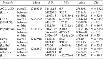
For all variables we use the available World Bank World Development Indicators data for 101 tropical countries from 1960 to 2009.Footnote 11 To aid comparison with previous results, we keep the same set of tropical countries as Barbier et al. (Reference Barbier, Damania and Léonard2005). The full list of countries can be found in appendix B, table 7, along with the table of summary statistics.
Comparison of equations (2)–(6) makes clear that – for our particular choice of model and explanatory variables – the profit-proportional and instantaneous-adjustment models can be nested within the ECM. Thus our base regression is the ECM from equation (4). Running the regression in logs to reduce the influence of outliers, we have
 $$\eqalign{\Delta ln(Ag.Land_{i,t}) &=\theta _{1}ln(Ag.Land_{i,t-1})+\gamma _{1}ln(GDPC_{i,t-1}) \cr &\quad+\beta _{1}\Delta ln(GDPC_{i,t}) +\gamma _{2}ln(Pop_{i,t-1}) \cr &\quad+\beta _{2}\Delta ln(Pop_{i,t})+\eta_{i}+\upsilon _{t}+\epsilon _{i,t}.}$$
While the country fixed-effects and year dummies do much to ameliorate omitted variable bias, there are two other sources of bias we might be concerned about. First, dynamic panel models contain an inherent bias (Nickell, Reference Nickell1981). Given the long time series (54 years), dynamic panel bias is not a major concern. Nevertheless, we provide Arellano–Bond estimates as a robustness check. A second source of bias is that agricultural land expansion will facilitate GDP growth, leading to simultaneity bias. To prevent this, the one- and two-year lag of GDP are used as instruments for the current and previous year, respectively.
4. Results
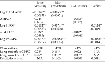
Table 1 presents the results of the four comparison specifications for the rate of change in agricultural land in our sample of tropical countries. The results, presented in table 1, provide evidence that there is an adjustment mechanism in the process of accumulating agricultural land. The coefficient on the lagged level of agricultural landholdings is significant in both the ECM and effort-proportional model. Further, the magnitude is similar in both models. The speed of adjustment to the new equilibrium is the negative of the coefficient on lagged agricultural land, around 0.017. This slow adjustment means that a short-run shock has long-lasting effects and provides initial evidence against the instantaneous-adjustment model.
Comparing a common ad hoc specification to those derived from three different assumptions about disequilibrium adjustment

Notes: Coefficient estimates from fixed-effects models. 2SLS instrument used for GDPC. Year dummies included but not reported. Robust standard errors in parentheses. Restrictions p-val reports the results of the Wald test of the constraints that the model implies for the error-correcting model. *p < 0.10, **p < 0.05, ***p < 0.01.
As explained in section 2, we can use the coefficient on lagged agricultural land to calculate the long-run elasticities of land area to income and population changes. These long-run estimates are presented at the bottom of table 1. Our two dynamic models in columns 1 and 2 suggest the long-run income elasticity is between 0.3 and 0.4. Given that average growth for a country in our data set is 3.8 per cent, income growth annually increases the predicted steady-state forest cover by 1–1.5 per cent. The long-run population elasticity is 1.05 according to the effort-proportional model and 0.95 according to the ECM. That is, for each 1 per cent increase in population, we have a 1 per cent increase in agricultural land area. Since average population growth over time for a country was 2.1 per cent, predicted steady-state forest cover falls by approximately 2 per cent each year.
Comparison of these long-run estimates with those of the instantaneous-adjustment model again highlights the importance of the dynamic specifications. The instantaneous-adjustment model underestimates the long-run income elasticity of agricultural land area by an order of magnitude, and population elasticity by a third, compared to the ECM and effort-proportional model.
Comparing the magnitude of the above estimates to those obtained from the instantaneous-adjustment and ad hoc models, we see that the implications of ignoring dynamics are not innocuous. The instantaneous-adjustment model assumes that the full long-run effect occurs in the first year – i.e., that short-run and long-run effects are equal. Thus it underestimates the long-run income elasticity of agricultural land area by an order of magnitude, and population elasticity by a third, compared to the ECM and effort-proportional model. We cannot estimate long-run effects from the ad hoc model as it is not a properly specified dynamic model.
The order-of-magnitude underestimation of the long-run income effects by the instantaneous-adjustment model can be easily understood with reference to the short-run effect estimated by the ECM. This effect is positive and of roughly the same magnitude as the long-run effects but with opposite sign.Footnote 12 The instantaneous-adjustment model is forced to estimate the combined effects with a single coefficient.
The inappropriateness of the restrictions implied by the instantaneous-adjustment and ad hoc models are further confirmed by Wald tests. These tests strongly reject the hypothesis that the coefficients on the additional variables in the ECM are equal to zero (see bottom of table 1). In contrast, the restrictions implied by the effort-proportional model cannot be rejected at the 15 per cent level.
4.1. Robustness checks
We undertake four robustness checks. The first is to restrict the sample to post-1980. The second is to use the Arellano Bond estimator. Thirdly, we add additional covariates. Lastly we allow for possible non-monotonic influence of per capita income.Footnote 13
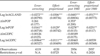
Using such a long data set is not without costs. For one, it is plausible that the deforestation in the 1960s was different from recent deforestation. It is also reasonable to argue that the quality of data was poorer in earlier years. Further, panel lengths are often 20–40 years; ours was over 50 (Bhattarai and Hammig, Reference Bhattarai and Hammig2004; Barbier et al., Reference Barbier, Damania and Léonard2005; López and Galinato, Reference López and Galinato2005; Nguyen Van and Azomahou, Reference Van Nguyen and Azomahou2007; Scrieciu, Reference Scrieciu2007; Arcand et al., Reference Arcand, Guillaumont and Jeanneney2008). Lastly, our model described in appendix A relies on the assumption of small, open economies. This means our model works best for the era of modern globalization, commonly thought to have begun around 1980 (Dollar, Reference Dollar2001; Aisbett, Reference Aisbett2005). Thus in table 2 we restrict the sample to the period since 1980.Footnote 14
Post 1980 sample comparing a typical ad hoc specification to those derived from three different assumptions about disequilibrium adjustment

Notes: Coefficient estimates from fixed-effects models. 2SLS instrument used for GDPC. Year dummies included but not reported. Robust standard errors in parentheses. Restrictions p-val reports the results of the Wald test of the constraints that the model implies for the error-correcting model.
*p < 0.10, ***p < 0.01.
The results in table 2 provide further evidence of the importance of accounting for gradual adjustment. Both the instantaneous and ad hoc specifications once again underestimate the ultimate impact of population and per capita income on deforestation. Indeed, the ad hoc specification identifies no statistically significant effects in the post-1980 sample. Furthermore, at the bottom of column 1 we see that the Wald tests of the restrictions implied by these two models can again be rejected at a 1 per cent level of significance.
Comparing these results with the full data set, we see evidence of a changed relationship in recent years. For the ECM model, the long-run elasticity of GDP increases from −0.2 to around 0 when we focus on the post-1980 sample. Meanwhile long-run population elasticity decreases from around 1 to around 0.5. This change comes from an increasing speed of adjustment to equilibrium. The magnitude of the coefficient on lagged agricultural land is three times larger in the post-1980 sample compared to the full sample.
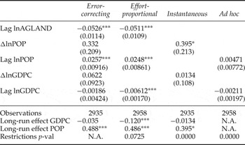
The second robustness check is to use the Arellano–Bond estimator for the two dynamic specifications. We apply the Arellano–Bond estimator to both the full and post-1980 samples (see table 3). The results are very similar to our estimates in table 1.Footnote 15 The similarity of the results using the two estimators confirms that our time series is long enough that Nickell bias is not a concern.
Arellano–Bond dynamic fixed-effects model estimates for both full and post-1980 samples

Notes: GDPC variables and lagged agricultural land instrumented. Year dummies included but not reported. Robust standard errors in parentheses. Restrictions p-val reports the results of the Wald test of the constraints that the model implies for the error-correcting model.
* p < 0.10, ** p < 0.05, *** p < 0.01.
Our next robustness check adds controls for cereal yield and length of road network. In our model, cereal yield maps to land productivity Z and we expects higher values of yield to increase deforestation. Increases in road network imply decreases in transportation cost T. For this reason, increases in the road network are commonly believed to raise deforestation.
The road network and cereal yield variables were not included in our base regression because a paucity of data leads to a significant reduction in sample size. Additionally, the road network is potentially highly endogenous–roads may be built by those wishing to establish property rights and extract both wood and agricultural produce from previously forested areas.
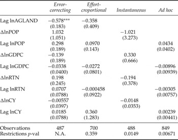
Despite these concerns, we present the results of the models including road length and cereal yield in table 4. In this table, the only statistically significant coefficient in any specification is the lagged agricultural land in the ECM. The reason for this loss of significance is likely due to the drastic reduction in sample size, and the need to instrument the length of roads variables along with the GDP variables.
Robustness to controlling for road length and cereal yield

Notes: Coefficient estimates from fixed-effects models. 2SLS instrument used for GDPC. Year dummies included but not reported. Robust standard errors in parentheses. Restrictions p-val reports the results of the Wald test of the constraints that the model implies for the error-correcting model.
*** p < 0.01.
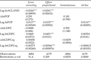
Until now, our modeling has reflected the assumption in our theoretical model in appendix A that changes in income per capita affect the rate of forest conversion only through changes in the alternative wage (in the non-agricultural sector) for potential settlers. This assumption leads to the prediction that increases in per capita income unambiguously decrease the rate of forest conversion. It is, however, perfectly possible that per capita income also affects demand for the products of forest conversion, raising returns to the activity. These two competing influences of per capita income on deforestation may lead to a non-monotonic relationship between the two. Our final robustness check allows for this possibility by adding the term(s) appropriate for a squared log of GDP per capita in each specification. The specifications essentially represent those typically associated with the Environmental Kuznets Curve. The results are in table 5. As was the case for all the previous checks, the Wald tests at the bottom of the table show that the restrictions imposed by the two static models are strongly rejected, while those imposed by the effort-proportional model are not. The signs on the per capita income terms are broadly consistent with the Kuznets-style inverted U-shaped relationship between per capita income and deforestation rate. However, the terms are only statistically significant with the expected sign in the effort-proportional model.
Robustness to allowing for non-monotonic influence of GDP per capita. Specifications are similar to Environmental Kuznet's Curve models

Notes: Coefficient estimates from fixed-effects models. 2SLS instrument used for GDPC. Year dummies included but not reported. Robust standard errors in parentheses. Restrictions p-val reports the results of the Wald test of the constraints that the model implies for the error-correcting model.
** p < 0.05, *** p < 0.01.
5. Conclusion
Much of the cross-country empirical literature on deforestation is open to the criticism of ad hoc time-series specification due to the regression of changes in forest cover on levels of explanatory variables. This paper responds to this criticism by developing three alternative regression models arising from three alternative assumptions about the adjustment process of deforestation to changes in underlying economic drivers. The first of these assumptions is that adjustment is instantaneous. While intuitively unlikely, this is the assumption which is implied by applying a standard, static model of deforestation and is sometimes used in the empirical literature.Footnote 16
The second assumption is that the rate of change in forest cover is proportional to the product of the number of settlers and the optimal deforesting effort of each. The optimal effort of each settler, in turn, depends on the profitability of clearing land and claiming property rights. This theoretically motivated assumption about the dynamics of deforestation leads to a specification which is very similar to the ad hoc practice commonly found in the literature of regressing changes in forest cover on levels of explanatory variables. There is, however, one important difference. Our theoretically motivated specification includes the lagged extent of already cleared land.
Our final, and least restrictive, assumption is simply that adjustment may happen with a lag. This assumption can be used to derive an unconstrained ECM of changes in forest cover.
Methodologically the main conclusion of our paper is that the implications of using an ad hoc empirical model, or one which assumes (implicitly or otherwise) instantaneous-adjustment, are not innocuous. Instantaneous adjustment assumes that the effect of last year's shocks do not influence this year's deforestation rates. The evidence provided in the paper supports a very different conclusion: that shocks continue to affect deforestation for many years. Furthermore, both the instantaneous-adjustment and ad hoc models consistently understate the total effect of income and population shocks on deforestation – sometimes by more than an order of magnitude.
Improving the dynamic specification of empirical models of deforestation also has policy benefits. A leading global initiative, REDD+, aims to provide compensation for deforestation rates below a reference level. A major difficulty is estimating this reference level. Our results motivate the use of forecasting methods: since most of the effect of a shock on deforestation rates occurs in the years after a shock, deforestation rates can plausibly be forecast with the appropriate dynamic specification.
Appendix A: Theory
The current paper argues quite simply that – for any given model of equilibrium forest cover – the assumptions made (implicitly or otherwise) about the rate of disequilibrium adjustment influence the choice of empirical model, and in turn the empirical results. We demonstrate this using a simple model based on that of Mendelsohn (Reference Mendelsohn1994). We chose this model specifically because its simplicity aids exposition and clarity. We hope that other researchers will apply our methodological insights to improve the empirical testing of the many other, more complex, models in the literature.
Mendelsohn's model is an example of a von Thünen model of land rents and frontier expansion by settlers (von Thünen and Hall, Reference von Thünen and Hall1966). We summarize here the relevant features of the model for ease of reference later. For a more detailed model description, the reader is referred to Mendelsohn (Reference Mendelsohn1994).Footnote 17
The model economy has three regions: at the center of each economy is a market, which is surrounded by agriculture, and forests beyond. For simplicity, land exists on a rectangular strip one unit wide.Footnote 18 The model focuses on determining the location of the extensive margin separating agriculture from forests. The location of the extensive margin is denoted by the distance to the frontier from the center, d. Hence the total area of agricultural land is 2d. There is only one type of agriculture and forests are assumed to have zero economic value. In the language of Angelsen (Reference Angelsen1999), we also assume a perfect labor market (such that labor may be bought or sold at a constant hourly wage rate, w), an exogenous number of settlers N, and a small, open economy (such that all prices are exogenous). It will be clear from the following that the final assumption is crucial, because with exogenous prices, the impact of GDP (and thus non-forestry wage) growth on deforestation is unambiguously negative.
Each hectare of land generates Z tonnes of output per year, which can be sold at exogenous price p dollars per tonne in markets. There are three types of costs associated with production. The first is transportation costs of T dollars per tonne per kilometer from farm to the city. The second are annual per hectare labor costs w, which can be purchased or settler provided. In the case of settler-provided labor, wages can be seen as the settler's reservation payoff. As the settler is interested in lifetime profits, the settler will calculate the present value of future profits over a settled hectare with the discount rate r.
The third input is the cost to the settler of establishing and maintaining property rights in the tradition of Demsetz (Reference Demsetz1964). Because the land has value in terms of returns from production, there is conflict over resources. We assume that each settler must initially invest resources, x i at cost c per unit, in creating his/her property right. Thereafter a settler must invest α per hectare per year to maintain these property rights.
With N identical settlers, each settler's share of the newly converted land is proportional to their share in property rights expenditure. Hence the area of land obtained after investing x
i
is
 $2\lpar x_{i}/\sum_{k=1}^{N} x_{k}\rpar $
. Let
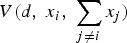 $V\lpar d\comma \; x_{i}\comma \; \sum_{j \neq i} x_{j}\rpar $
be the present value of that land, then
 $$ {V(d,x_{i},\sum_{j\neq i}x_j)}=\displaystyle{{(pZ - w - Td - \alpha)}\over{r}} \displaystyle{{x_{i}}\over{\sum_{k=1}^N x_{k}}}-cx_{i}.$$
The amount of resources spent in equilibrium for land at distance d from the city can be solved by choosing x i to maximize (8), holding other settlers' expenditure constant. This gives the implicit solution to the optimal investment in property rights as
 $$\eqalign{\displaystyle{{2(pZ-w-Td-\alpha )}\over{r}}=\displaystyle{{c\left( \sum_{k=1}^{N}x_{k}^{\ast}\right) ^{2}}\over{\sum_{k=1}^{N}x_{k}^{\ast }-x_{i}^{\ast }}},}$$
from which we can obtain the explicit solution by assuming all settlers are alike,
 $$x^{\ast }(d,N)=\displaystyle{{(pZ-w-Td-\alpha )}\over{rc}} \displaystyle{{(N-1)}\over{N^{2}}}.$$
As N is exogenous, we only need to define the forest frontier to close the model. The forest frontier is defined by the distance from the center of either leading edge of the rectangular strip of land at which there is no incentive for agents to expend resources to establish property rights.Footnote
19
That is,
 $x^{\ast }\lpar d_{max}\comma \; N\rpar =0$
. From this we can solve for the maximum distance to the frontier,
 $$d_{max}=\displaystyle{{pZ-w-\alpha}\over{T}}.$$
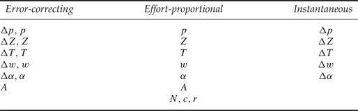
Equation (10) provides simple, clear predictions over the long-run position of the frontier, and thus area of agricultural land 2d max . Output prices and yields (p, Z) increase the distance of the frontier to market, whereas wages, ongoing property rights enforcement costs and transportation costs (w,α, T) decrease the area under agriculture. At equilibrium the costs of clearing do not affect the location of the forest frontier.Footnote 20
Relevant parameters for change in forest (or agricultural) land suggested by the model

Appendix B: Data
List of countries:
Angola, American Samoa, Burundi, Benin, Burkina Faso, Bangladesh, The Bahamas, Belize, Bolivia, Brazil, Barbados, Brunei Darussalam, Bhutan, Botswana, Central African Republic, Cote d'Ivoire, Cameroon, Republic of the Congo, Colombia, Comoros, Costa Rica, Cuba, Dominica, Dominican Republic, Ecuador, Eritrea, Ethiopia, Fiji, Gabon, Ghana, Guinea, The Gambia, Guinea-Bissau, Equatorial Guinea, Grenada, Guatemala, Guam, Guyana, Honduras, Haiti, Indonesia, India, Jamaica, Kenya, Cambodia, St. Kitts and Nevis, Lao PDR, Liberia, St. Lucia, Sri Lanka, Morocco, Madagascar, Maldives, Mexico, Mali, Myanmar, Mozambique, Mauritania, Mauritius, Malawi, Malaysia, Namibia, New Caledonia, Niger, Nigeria, Nicaragua, Nepal, Pakistan, Panama, Peru, Philippines, Papua New Guinea, Puerto Rico, Paraguay, French Polynesia, Rwanda, Sudan, Senegal, Singapore, Solomon Islands, Sierra Leone, El Salvador, Somalia, Sao Tome and Principe, Suriname, Seychelles, Chad, Togo, Thailand, Tonga, Trinidad and Tobago, Tanzania, Uganda, St. Vincent and the Grenadines, Venezuela RB, Vietnam, Vanuatu, Samoa, Democratic Republic of the Congo, Zambia, Zimbabwe
Summary statistics