1. Introduction
What was the role of the changing impact of monetarism on policy behavior? How did these changes shape US macroeconomic dynamics during the 1970s? To examine these questions, I develop a business cycle model where money is allowed (but not required) to play a role in determining the equilibrium values of inflation and output. Nonzero steady-state trend inflation is incorporated to account for the evolution of inflation observed in the data.
I use numerical techniques to compute the determinacy conditions required for a rational expectation equilibrium (REE). These conditions illustrate regions where the central bank can specifically rule out self-fulfilling expectations-driven fluctuations, that is, satisfy the “Taylor principle.” As noted by Kiley (Reference Kiley>2007) and Ascari and Ropele (Reference Ascari and Ropele>2009), an increasingly higher response to inflation is required by the central bank to achieve a determinate REE for even low levels of trend inflation. I show that augmenting a standard interest rate rule with money enables the central bank to achieve price determinacy for trend inflation as high as 5% in the New-Keynesian trend inflation model compared to below 2% in a Taylor-type policy rule. The full model with money and varying levels of trend inflation reduces the likelihood of price determinacy even when the central bank responds reasonably strongly to money growth.
To empirically extract the historical likelihood of determinacy, I estimate a monetary policy reaction function for the Fed before and after Volcker’s disinflation. I use novel real-time data on money aggregates to estimate this rule, an approach in line with Orphanides (Reference Orphanides>2001, Reference Orphanides>2002, Reference Orphanides>2003), Boivin (Reference Boivin>2006), Coibion and Gorodnichenko (Reference Coibion and Gorodnichenko>2011). My main empirical results suggest that money aggregate M1 entered the Fed’s reaction function during the pre-Volcker period and became statistically indistinguishable from zero starting Volcker’s disinflation. These results are consistent with those offered by Sims and Zha (Reference Sims and Zha>2006), Castelnuovo (Reference Castelnuovo>2012), in that money played an important role in shaping monetary policy during the pre-Volcker era. Monetary policy changed in other important ways: while the response to inflation was statistically indistinguishable from the threshold value of one in the pre-Volcker period, it became larger in the post-Volcker sample; the coefficient on output gap is gradually reduced over time, while policy became more inertial.
I combine the empirical distribution of my parameter estimates of the policy rule with a calibrated New-Keynesian model to test the likelihood of price indeterminacy under various levels of trend inflation. Even though money aggregate M1 enters positively and significantly in the Fed’s reaction function, the response was likely not sufficient to insulate the US economy from self-fulfilling fluctuations during the pre-Volcker era. The change in the response to inflation and the reduction in trend inflation explain almost entirely the move from an indeterminate region to a determinate one. The likelihood of a determinate equilibrium is low when money is allowed to enter via non-separability and portfolio adjustment costs. The case for indeterminacy during the pre-Volcker period weakens when non-separability between consumption and real balances, and portfolio adjustment costs are excluded from the model, due to the large estimated response to money. The findings suggest non-separable utility, adjustment costs, and money in the policy rule within a positive trend inflation environment are important to fully capture the role of monetarism in shaping macroeconomic dynamics during the pre-Volcker period. The overall findings generally support the conclusions of Clarida et al. (Reference Clarida, Gali and Gertler>2000) and Coibion and Gorodnichenko (Reference Coibion and Gorodnichenko>2011) by specifically including a role for money.
The paper contributes to three strands of the literature. I generalize the findings of Keating and Smith (Reference Keating and Smith>2013) by including a role for trend inflation and by allowing money to play a role, extending the work of Kurozumi (Reference Kurozumi>2006) who studies the role of non-separability in driving determinacy in a model without trend inflation. The results extend the theoretical literature on price-level determinacy (Taylor (Reference Taylor>1999), Bullard and Mitra (Reference Bullard and Mitra>2002), Woodford, (Reference Woodford>2011), and Galí, (Reference Galí>2015)).
The key empirical innovation rests on the use of real-time data on money aggregates, an approach in line with Orphanides (Reference Orphanides>2001, Reference Orphanides>2002, Reference Orphanides>2003), Boivin (Reference Boivin>2006), and Coibion and Gorodnichenko (Reference Coibion and Gorodnichenko>2011). Because money growth aggregates are not readily available at the meeting level, I compile data on money aggregates M1 using the briefing forecasts prepared for the FOMC, included in the Greenbook. The results formalize the role of money in the FOMC policy reaction function (Sims and Zha (Reference Sims and Zha>2006), Chowdhury and Schabert (Reference Chowdhury and Schabert>2008), Li et al., (Reference Li, Liu and Pei>2020), Castelnuovo (Reference Castelnuovo>2012), present a description of the monetary reaction function during the Great Inflation using real-time data (Clarida et al. (Reference Clarida, Gali and Gertler>1998), Orphanides, (Reference Orphanides>2001, Reference Orphanides>2002, Reference Orphanides>2003), Boivin, (Reference Boivin>2006), Chowdhury and Schabert (Reference Chowdhury and Schabert>2008), Coibion and Gorodnichenko (Reference Coibion and Gorodnichenko>2011), Hirose et al. (Reference Hirose, Kurozumi and Van Zandweghe>2020), Li et al. (Reference Li, Liu and Pei>2020)), and formalize the role of money in describing historical US monetary policy (Ireland (Reference Ireland>2004), Favara and Giordani (Reference Favara and Giordani>2009), Canova and Menz (Reference Canova and Menz>2011), Qureshi (Reference Qureshi>2016, Reference Qureshi>2018, Reference Qureshi>2020), Li et al., (Reference Li, Liu and Pei>2020)).
The conclusions explain the dramatic rise in inflation experienced by the US economy during the 1960s and 1970s, followed by a substantial reduction in the 1980s. Clarida et al. (Reference Clarida, Gali and Gertler>2000) suggest that the inability of the US Federal Reserve (“the Fed”) to raise nominal interest rates more than one-for-one with inflation—that is, to satisfy the (Taylor (Reference Taylor>1999)) principle—induced self-fulfilling expectations-driven fluctuations, causing indeterminacy, which was reversed under the chairmanship of Paul Volcker in 1979. Their findings are sensitive to the data employed: Orphanides, (Reference Orphanides>2001, Reference Orphanides>2002, Reference Orphanides>2003) using FOMC meeting-level data does not detect large changes in the Fed’s response to inflation when comparing the period before and after Volcker’s appointment. Combining the trend inflation framework of Kiley (Reference Kiley>2007) and Ascari and Ropele (Reference Ascari and Ropele>2009) with meeting-level data, Coibion and Gorodnichenko (Reference Coibion and Gorodnichenko>2011) find that the policy response combined with positive trend inflation recovers the main results of Clarida et al. (Reference Clarida, Gali and Gertler>2000). Sims and Zha (Reference Sims and Zha>2006) include money in their empirical framework but do not account for real-time data or trend inflation, both of which are central to generating the indeterminacy outcomes of Coibion and Gorodnichenko (Reference Coibion and Gorodnichenko>2011).
The next section outlines the model. Section 3 presents the determinacy conditions implied by a monetary policy rule with money growth. Section 4 presents empirical evidence of money growth in the reaction function and combines these results with the analytical framework to study the implications on price determinacy. Section 5 concludes the paper.
2. The model
I derive a New-Keynesian model with positive trend inflation developed by Ascari (Reference Ascari>2004), Ascari and Ropele (Reference Ascari and Ropele>2009), Ascari and Sbordone (Reference Ascari and Sbordone>2014) with a model where money is allowed (but not required) to play a role (Nelson (Reference Nelson>2002), Ireland, (Reference Ireland>2004), Andrés et al. (Reference Andrés, López-Salido and Nelson>2009)).
2.1. Description of the non-linear DSGE model
The household portion of the paper works with the DSGE model developed by Nelson (Reference Nelson>2002), Ireland (Reference Ireland>2004), Andrés et al. (Reference Andrés, López-Salido and Nelson>2009). The economy consists of a continuum of households, with the representative household maximizing the following objective function:
 \begin{equation} \max _{C_{t},N_{t},M_{t},B_{t}}E_{0}\sum _{t = 0}^{\infty }\beta ^{t}a_{t}\left [\Psi \!\left (C_{t,h},\frac{M_{t}}{e_{t} P_{t}}\right )-\frac{N_{t}^{1+\varphi }}{1+\varphi }-G\!\left (\bullet \right )\right ] \end{equation}
where
 $C_{t,h}$
is the quantity consumed of the differentiated goods and allows for (internal) habit formation (
 $h$
),
 $C_{t,h}=\frac{C_{t}}{C_{t-1}^{h}}$
, to account for the gradual response of output to monetary policy shocks (Fuhrer (Reference Fuhrer>2000)), real money balances are denoted by
 $\frac{M_{t}}{P_{t}}$
, and
 $N_{t}$
denotes labor hours or employment. Moreover,
 $a_{t}$
is a preference shock,
 $e_{t}$
is a shock to household’s demand for real balances,
 $\beta \in (0,1)$
is the discount factor,
 $\Psi$
can be interpreted as the intra-temporal non-separability between consumption and real balances, making it possible to test the relevance of an explicit money-balance term in the equations determining supply and demand decisions, and
 $\varphi$
represents the inverse of the Frisch labor elasticity.
The term,
 $G\!\left (\bullet \right )=\frac{d}{2}\!\left [\exp \!\left \{ c\!\left (\frac{M_{t}/P_{t}}{M_{t-1}/P_{t-1}}-1\right )\right \} +\exp \!\left \{ -c\!\left (\frac{M_{t}/P_{t}}{M_{t-1}/P_{t-1}}-1\right )\right \} -\!2\right ]$
, denotes portfolio adjustment costs, with
 $c,d \gt 0$
. As noted by Andrés et al. (Reference Andrés, López-Salido and Nelson>2009), the functional form for portfolio adjustment costs is modified to include real balances and applied to a model without “limited participation” features. The presence of portfolio adjustment costs implies substantial effects on money demand dynamics by making the demand for money a forward-looking equation, formalizing that expectations of interest rates matter for money demand, lagged dependent variable enter positively in the money demand function, and distinguishes between a long-run interest elasticity of money demand.Footnote 1 Maximization of the utility function in equation (1) is subject to a sequence of flow budget constraints given by:
 \begin{equation} \frac{M_{t-1}+B_{t-1}+W_{t}N_{t}+T_{t}}{P_{t}}=C_{t}+\frac{B_{t}/i_{t}+M_{t}}{P_{t}} \end{equation}
for
 $t = 0,1,2,\cdots$
where
 $P_{t}$
is the price of the consumption good,
 $W_{t}$
denotes the nominal wage,
 $B_{t}$
represents the quantity of one-period, nominally risk-less discount bonds purchased in period
 $t$
and maturing in period
 $t+1$
. Each bond pays one unit of money at maturity and its price is
 $1/i_{t}$
.
 $T_{t}$
represents lump-sum additions or subtractions to period income.
The supply side of the model follows closely the positive trend inflation framework developed by Ascari (Reference Ascari>2004), Ascari and Ropele (Reference Ascari and Ropele>2009), Ascari and Sbordone (Reference Ascari and Sbordone>2014). The final good,
 $Y_{t}$
, is produced by a perfectly competitive firm that aggregates intermediate goods
 $(Y_{i,t})$
produced by a continuum of monopolistically competitive firms. The optimal demand for intermediate inputs by final goods producer is equal to
 $Y_{i,t} = (P_{i,t}/P_{t})^{-\varepsilon } Y_{t}$
. Aggregate consumption equals production of final goods:
 \begin{equation} C_{t} = Y_{t} = \bigg [\int _{0}^{1} Y_{i,t}^{\frac{\varepsilon -1}{\varepsilon }} di \bigg ]^{\frac{\varepsilon }{\varepsilon -1} } \end{equation}
where
 $\varepsilon$
indicates the elasticity of substitution among the intermediate goods. The production function of intermediate goods producers is
 $ Y_{i,t} = z_{t} N^{1-\alpha }_{i,t}$
, where
 $z_{t}$
is an exogenous and stationary process for the level of technology. Based on Calvo (Reference Calvo>1983), in each period an intermediate firm can re-optimize its nominal price, denoted by
 $P^{\ast}_{i,t}$
, with a fixed probability
 $1-\theta$
, while with probability
 $\theta$
it can index its price to the previous period’s inflation rate.
 $P_{i,t} = \pi ^{\varrho }_{t}P_{i,t-1}$
which is based on Christiano et al. (Reference Christiano, Eichenbaum and Evans>2005), where the parameter
 $\varrho \in [0,1]$
indicates the degree of price indexation to past inflation, and
 $\pi _t = P_{t}/P_{t-1}$
is the inflation rate. The firm indexes inflation to past inflation only. The problem of the firm
 $i$
, which sets its price at time
 $t$
, is to choose
 $P^{\ast}_{i,t}$
to maximize expected profits:
 \begin{equation} E_{t}\sum _{j = 0}^{\infty } \theta ^{j}D_{t,t+j}\bigg [\frac{P^{\ast}_{i,t}\Pi ^{\varrho }_{t-1,t+j-1}}{P_{t+j}}Y_{i,t+j} - \frac{W_{t+j}}{P_{t+j}} \bigg (\frac{Y_{i,t+j}}{Z_{t+j}}\bigg )^{\frac{1}{1-\alpha }} \bigg ] \end{equation}
The firm maximizes revenue subject to the following demand constraint:
 \begin{equation} Y_{i,t+j} = \bigg (\frac{P^{\ast}_{i,t}\Pi ^{\varrho }_{t-1,t+j-1}}{P_{t+j}}\bigg )^{-\varepsilon } Y_{t+j} \end{equation}
 $D_{t,t+j} = \beta ^{j}\frac{\lambda _{t+j}}{\lambda _{0}}$
is the stochastic discount factor, with
 $\lambda _{t+j}$
denoting the
 $t+j$
marginal utility of consumption and
 $\Pi _{t,t+j}$
indicates the cumulative inflation between periods
 $t$
and
 $t+j$
:
 \begin{equation} \Pi _{t,t+j}=\left \{\begin{array}{l@{\quad}l} 1 \qquad & \textrm{if}\;\; j=0\\[5pt] \bigg (\frac{P_{t+1}}{P_{t}}\bigg ) \times \bigg (\frac{P_{t+2}}{P_{t+1}}\bigg ) \times \cdots \times \bigg (\frac{P_{t+j}}{P_{t+j-1}}\bigg ) & \textrm{if}\;\; j\gt 0 \end{array}\right. \end{equation}
The real marginal cost of firm
 $i$
is
 $MC_{i,t} = \frac{z^{\frac{1}{1-\alpha }}_{t}}{1-\alpha }{W_{t}}/{P_{t}}[({P_{i,t}}/{P_{t}})^{-\varepsilon }Y_{t}]^{\frac{\alpha }{1-\alpha }}$
, which depends on the quantity produced by the firm and features decreasing returns to scale. Since firms charging different prices would produce different levels of output, they have heterogeneous marginal costs. Prices are staggered because firms re-setting prices in different periods will set different prices. Then, in each given period
 $t$
, there will be a distribution of different prices. Price dispersion results in an efficiency loss in aggregate production.
 \begin{equation} N^d_{t} = \int _{0}^{1} N^d_{i,t}di = \int _{0}^{1} \bigg (\frac{P_{i,t}}{P_{t}}\bigg )^\frac{-\varepsilon }{1-\alpha } di \bigg (\frac{Y_{t}}{z_{t}}\bigg )^\frac{1}{1-\alpha } = s_{t}\bigg (\frac{Y_{t}}{z_{t}}\bigg )^\frac{1}{1-\alpha } \end{equation}
Schmitt-Grohé and Uribe (Reference Schmitt-Grohé and Uribe>2007) shows that
 $s_{t}$
is bounded below at one and represents the resource costs (or inefficiency loss) due to the relative price dispersion under the Calvo mechanism: for higher value of
 $s_{t}$
, more labor is needed to produce a given level of output.
2.2. The symmetric equilibrium
I derive the log-linearized version of the DSGE model with money and trend inflation.Footnote 2 Equation (8) is the Euler condition, which arises from the household’s optimal inter-temporal allocation of wealth and captures the negative relationship between output and the real-interest rate. This is determined by the difference between the nominal interest rate,
 $\hat{i}_{t}$
, and expected inflation,
 $E_{t}\hat{\pi }_{t+1}$
. Due to the inter-temporal substitution effect, higher real returns induce greater savings, depressing aggregate demand. Expectations of positive deviations in output expand current output. In the case when
 $\psi _{2} \neq 0$
, real balances enter the IS curve both contemporaneously, as well as in expectations. Therefore, non-separability across consumption and real balances makes the marginal utility of consumption a function of the amount of real balances optimally demanded by the households. This effect is amplified due to habit formation in consumption, which links real balances and lagged consumption.
 \begin{equation} \begin{aligned} \hat{y}_{t}= \frac{\phi _{1}}{\phi _{1}+\phi _{2}}\hat{y}_{t-1}+\frac{\beta \phi _{1}+\phi _{2}}{\phi _{1}+\phi _{2}}E_{t}\hat{y}_{t+1}-\frac{1}{\phi _{1}+\phi _{2}}\left (\hat{i}_{t}-E_{t}\hat{\pi }_{t+1}\right )-\frac{\beta \phi _{1}}{\phi _{1}+\phi _{2}}E_{t}\hat{y}_{t+2}\\[5pt] + \frac{\psi _{2}}{\psi _{1}(1-\beta h)(\phi _{1}+\phi _{2})}(\hat{m}_{t} - \hat{e}_{t}) - \frac{\psi _{2}(1+\beta h)}{\psi _{1}(1-\beta h)(\phi _{1}+\phi _{2})}(\hat{m}_{t+1} - \hat{e}_{t+1})\\[5pt] + \frac{\psi _{2}\beta h}{\psi _{1}(1-\beta h)(\phi _{1}+\phi _{2})}(\hat{m}_{t+2} - \hat{e}_{t+2})+\frac{\left (1-\beta h\rho _{a}\right )\left (1-\rho _{a}\right )}{\left (1-\beta h\right )\left (\phi _{1}+\phi _{2}\right )}\hat{a}_{t} \end{aligned} \end{equation}
The money demand equation (9) features output lags and leads, contemporaneous opportunity cost of holding money, and expected future real balances, with the coefficients
 $\gamma _{1}$
and
 $\gamma _{2}$
representing the long-run real-income and interest rate response parameters.Footnote 3 Allowing for non-separability across real balances and consumption gives real balances an explicit role in both the output and inflation equilibrium relationships. However, money continues to exert this role and remains dynamic even in the presence of separability (
 $\psi _{2} = 0$
) owing to nonzero portfolio adjustment costs (
 $\delta _{0} \gt 0$
). A key difference between the money demand curve derived here and those considered in Ireland (Reference Ireland>2004), Andrés et al. (Reference Andrés, López-Salido and Nelson>2009), Castelnuovo (Reference Castelnuovo>2012) is the inclusion of trend inflation, which directly affects the coefficients of the money demand curve, including the semi-elasticity of output and interest rates. High trend inflation has a direct bearing on the semi-elasticity of interest rate due to its effect on
 $\gamma _{2}$
.
 \begin{equation} \begin{aligned} \left [1 +\delta _{0}\!\left (1+\beta \right )\right ]\hat{m}_{t}= \gamma _{1}\hat{y}_{t}-\gamma _{2}\hat{i}_{t}+ \left [\gamma _{2}\!\left (\bar{r}-1\right )\left (h\phi _{2}-\phi _{1}\right )-h \gamma _{1}\right ]\hat{y}_{t-1}\\[5pt] -\gamma _{2}\!\left (\bar{r}-1\right )\beta \phi _{1}E_{t}\hat{y}_{t+1}+\delta _{0}\hat{m}_{t-1} +\left [\frac{\psi _{2}\!\left (\bar{r}-1\right )\beta h\gamma _{2}}{\psi _{1}\!\left (1-\beta h\right )}+\delta _{0}\beta \right ]\!E_{t}\hat{m}_{t+1}\\[5pt] -\frac{\left (\bar{r}-1\right )\beta h\!\left (1-\rho _{a}\right )}{1-\beta h}\gamma _{2}\hat{a}_{t} +\left \{1-\left (\bar{r}-1\right )\gamma _{2}\!\left [\frac{\psi _{2}\beta h\rho _{e}}{\psi _{1}\left (1-\beta h\right )}+1\right ]\right \}\!\hat{e}_{t} \end{aligned} \end{equation}
Turning to the supply side of the model, the positive steady-state inflation rate,
 $\bar{\Pi }$
, affects all coefficients in the Generalized New-Keynesian Phillips Curve (GNKPC) in equation (10). Two effects come into play in the positive trend inflation environment that are not present in the textbook version of the New-Keynesian model. When intermediate firms are free to adjust prices, they will set higher prices to try to offset the erosion of relative prices and profits that trend inflation automatically creates. Second, expectation of forward-looking terms is progressively multiplied by larger discount factors. This means that optimal price-setting under trend inflation reflects future economic conditions more than short-run cyclical variations and price-setting firms become more forward-looking. These two features have broad consequences for macroeconomic dynamics. Kiley (Reference Kiley>2007) and Ascari and Ropele (Reference Ascari and Ropele>2009) show that positive trend inflation substantially alters the determinacy region, requiring a larger response to inflation even for trend inflation levels as low as 2%. Indexation,
 $\hat{\Delta }_{t} = \hat{\pi }_{t}-\varrho \hat{\pi }_{t-1}$
mitigates these two effects.
 \begin{equation} \begin{aligned} \Gamma \hat{\Delta }_{t} = [1-\theta \bar{\Pi }^\frac{{\varepsilon (1-\varrho )}}{1-\alpha }]\hat{mc}_{t}\\[5pt] +\; \theta \beta \Theta (\beta \phi _{1}E_{t}\hat{y}_{t+1}+(1-\phi _{2})\hat{y}_{t} + \phi _1 \hat{y}_{t-1})+\theta \beta \Theta \hat{\tau }_{t} \\[5pt] +\;\theta \beta \left [\bar{\Pi }^\frac{{\varepsilon (1-\varrho )}}{1-\alpha }\left (\Gamma +\frac{\varepsilon }{1-\alpha }\right ) - (\varepsilon -1)\bar{\Pi }^{(\varepsilon -1)(1-\varrho )}\right ]\hat{\Delta }_{t+1}\\[5pt] +\;\theta \beta \Theta \left [\left (\frac{1-\beta h \rho _{a}}{1-\beta h}\right )\hat{a}_{t}+ \frac{\psi _{2}}{\psi _{1}(1-\beta h)}(\hat{m}_{t}-\hat{e}_{t}) - \frac{\beta h \psi _{2}}{\psi _{1}(1-\beta h)}(\hat{m}_{t+1}-\hat{e}_{t+1})\right ] \end{aligned} \end{equation}
In equation (10), the marginal cost,
 $\hat{mc}_{t}$
, which includes real balances due to the assumption of non-separability in the utility function, can be written as:
 \begin{equation} \begin{aligned} \hat{mc}_{t} & = (\chi +\phi _{2})\hat{y}_{t}-\phi _{1}\hat{y}_{t-1} -\beta \phi _{1}\hat{y}_{t-1} - \frac{\psi _{2}}{\psi _{1}(1-\beta h)}(\hat{m}_{t}-\hat{e}_{t})\\[5pt] & \quad + \frac{\beta h \psi _{2}}{\psi _{1}(1-\beta h)}(\hat{m}_{t+1}-\hat{e}_{t+1})-\frac{\beta h (1-\rho _a)}{1-\beta h}\hat{a}_{t} - (1+\chi )z_{t} \end{aligned} \end{equation}
The model with trend inflation and money is markedly different from the models that include only trend inflation or only money. In the current specification, real balances affect inflation directly and through marginal cost because real balances affect the household labor supply decision and, hence, in equilibrium, real wages. An alternative interpretation of money in the NKPC is the cost channel of inflation mechanism, with money acting as a proxy for interest rates (Ravenna and Walsh (Reference Ravenna and Walsh>2006), Andrés et al.(Reference Andrés, López-Salido and Nelson>2009), Castelnuovo (Reference Castelnuovo>2012), aligning the model with the cost channel and trend inflation dynamics discussed in Qureshi and Ahmad (Reference Qureshi and Ahmad>2021). The Phillips Curve is also affected by an auxiliary process,
 $\hat{\tau }_{t}$
which also includes forward-looking inflation and therefore, also participates in the determination of inflation.
 \begin{equation} \begin{aligned} \hat{\tau }_{t} &= \Lambda \left [\left (\frac{1-\beta h \rho _{a}}{1-\beta h}\right )\hat{a}_{t}+ \frac{\psi _{2}}{\psi _{1}(1-\beta h)}(\hat{m}_{t}-\hat{e}_{t}) - \frac{\beta h \psi _{2}}{\psi _{1}(1-\beta h)}(\hat{m}_{t+1}-\hat{e}_{t+1})\right ]\\[5pt] & \quad + \Lambda (\beta \phi _{1}E_{t}\hat{y}_{t+1}+(1-\phi _{2})\hat{y}_{t} + \phi _1 \hat{y}_{t-1}) +(1-\Lambda )[E_{t}\hat{\tau }_{t+1} + (\varepsilon -1)\hat{\Delta }_{t+1}] \end{aligned} \end{equation}
The NKPC is influenced by the price dispersion process,
 $\hat{s}_{t}$
, that arises due to the assumption of Calvo pricing. Positive trend inflation implies that this term is relevant in the first order and affects the evolution of the log-linearized inflation rate as follows:
 \begin{equation} \hat{s}_{t} = \frac{\varepsilon }{1-\alpha }\Omega \hat{\Delta }_{t} + \theta \bar{\Pi }^\frac{{\varepsilon (1-\varrho )}}{1-\alpha }\hat{s}_{t-1} \end{equation}
The model is closed by adding a monetary policy reaction function to describe the actions of the central bank. I consider a specification that includes money growth in addition to the features of the baseline Taylor rule that typically include inflation and the output gap. As argued by Andrés et al. (Reference Andrés, López-Salido and Nelson>2009), an interest rate rule that includes money growth (or the change in real balances) might be rationalized, as in Svensson (Reference Svensson>1999), as part of an optimal reaction function when money growth variability appears in the central bank’s loss function. Under non-separability, as the central bank minimizes its loss function, at least with respect to inflation, its optimization problem implies that money enters the monetary policy rule automatically (see, for instance, the discussion in Woodford (Reference Woodford>2011)). Söderström, (Reference Söderström>2005) demonstrates how a target for money growth can be beneficial for an inflation-targeting central bank acting under discretion. Alternatively, the response to money might be rationalized by money’s usefulness in forecasting inflation. A similarly specified rule has been estimated in Ireland (Reference Ireland>2004), Andrés, et al. (Reference Andrés, López-Salido and Nelson>2009), Canova and Menz (Reference Canova and Menz>2011), Qureshi (Reference Qureshi>2016), Li et al. (Reference Li, Liu and Pei>2020), Qureshi (Reference Qureshi>2020), Castelnuovo (Reference Castelnuovo>2012) that captures the forward-looking behavior of the Fed can be written as follows (with
 $j$
denoting forecast horizons):
 \begin{equation} \hat{i}_{t} = \rho _{1,t}\hat{i}_{t-1}+ \rho _{2,t}\hat{i}_{t-2}+(1-\rho _{1,t}- \rho _{2,t})[\psi _{\pi,t}E_{t}\hat{\pi }_{t+j}+\psi _{x,t}E_{t}\hat{y}_{t+j}+\psi _{\mu,t}E_{t} \hat{\mu }_{t+j}]+cons_{t}+\epsilon _{t} \end{equation}
for
 $j \in \{0,1,\cdots \}$
,
 $\epsilon _{t}$
is an error term, and the time-varying constant term includes the (possibly time-varying) targets for inflation (
 $\bar{\pi }_{t}$
), output gap (
 $\bar{y}_{t}$
), money growth (
 $ \bar{\mu }_{t}$
), and the real-interest rate (
 $r_{t}$
), given by:
 \begin{equation} cons_{t} = (1-\rho _{1,t}- \rho _{2,t})[(1-\psi _{\pi,t})\bar{\pi }_{t}+ r_{t} - \psi _{\mu,t}\Delta \bar{\mu }_{t} - \psi _{x,t}\bar{y}_{t}) \end{equation}
2.3. Model parameters and calibration
The compound parameters
 $\psi _{1}$
,
 $\psi _{2}$
,
 $\phi _{1}$
,
 $\phi _{2}$
,
 $\delta _{0}$
,
 $\Lambda$
,
 $\chi$
,
 $\Theta$
,
 $\Gamma$
,
 $\Omega$
,
 $\gamma _{1}$
, and
 $\gamma _{2}$
are convolutions of deeper parameters, including the structural parameters and possibly time-invariant parameters, such as trend inflation. Note first that gross inflation,
 $\bar{\Pi } = 1$
(or full indexation,
 $\varrho = 1$
) shuts down the trend inflation portion of the model through the parameters
 $\Lambda$
,
 $\Gamma$
,
 $\Omega$
, and
 $\Theta$
that enter the GNKPC and returns the model of Andrés et al. (Reference Andrés, López-Salido and Nelson>2009). Setting non-separability
 $\psi _2 = 0$
, portfolio adjustment costs
 $\delta _{0}=0$
, and
 $\psi _{\mu } = 0$
shuts down the money portion of the model (model without money) and returns the frameworks of Ascari et al. (Reference Ascari, Castelnuovo and Rossi>2011). The parameters
 $\gamma _{1}$
and
 $\gamma _{2}$
are the semi-elasticity of output and interest, respectively. Shutting down both trend inflation and money features returns the textbook New-Keynesian model presented in Galí (Reference Galí>2015).
 \begin{align*} \psi _{1} &= -\frac{\Psi _{1}}{\bar{y}^{1-h} \Psi _{11}} & \psi _{2} &= -\frac{\Psi _{12}}{\bar{y}^{1-h} \Psi _{11}}\frac{\bar{m}}{\bar{e}}\\[5pt] \phi _{1} &=\frac{(\psi ^{-1}-1)h}{1-\beta h} & \phi _{2} &= \frac{\psi ^{-1} + (\psi ^{-1}-1)\beta h^2 - \beta h}{1-\beta h} \\[5pt] \Lambda &= 1-\theta \beta \bar{\Pi }^{(\varepsilon -1)(1-\varrho )} & \chi &= \frac{\varphi +\alpha }{1 - \alpha } \\[5pt] \gamma _{1} &= \gamma _{2}\left [\bar{r}\frac{\bar{y}}{\bar{m}} \frac{\psi _2}{\psi _1}\frac{1}{1-\beta h} + (\bar{r}-1)\phi _2\right ]& \gamma _{2}(\bar{r}-1) &=\left [\frac{\Psi _{2}}{\Psi _2 \frac{\psi _2}{\psi _1}\frac{1}{1-\beta h} - \Psi _{22} \frac{\bar{m}}{\bar{e}}} \right ]\\[5pt] \Gamma &= \left (1+\frac{\varepsilon \alpha }{1-\alpha }\right )\frac{\theta \bar{\Pi }^{(\varepsilon -1)(1-\varrho )}}{1-\theta \bar{\Pi }^{(\varepsilon -1)(1-\varrho )}} & \Theta &= \left [\bar{\Pi }^{(\varepsilon -1)(1-\varrho )} - \bar{\Pi }^\frac{{\varepsilon (1-\varrho )}}{1-\alpha }\right ]\\[5pt] \Omega &= \left [\theta \bar{\Pi }^\frac{{\varepsilon (1-\varrho )}}{1-\alpha } - \left (1-\theta \bar{\Pi }^\frac{{\varepsilon (1-\varrho )}}{1-\alpha }\right ) \frac{\theta \bar{\Pi }^{(\varepsilon -1)(1-\varrho )}}{1-\theta \bar{\Pi }^{(\varepsilon -1)(1-\varrho )}}\right ] & \delta _0 &= -\frac{c^2 d}{\Psi _{22} \bar{m}^2} \end{align*}
To focus on the consequences of money growth targeting in this framework, I rely on numerical techniques using calibrated versions of the model, enabling me to compute the determinacy regions required for a rational expectations equilibrium (REE). In the numerical exercises, I vary the level of trend inflation to extract the role of policy in determining a REE, further generating determinacy regions for various features of the model with money. Therefore, determinacy in this model extends the baseline case of the model presented in Galí (Reference Galí>2015) and builds on the role played by trend inflation in altering the determinacy region—as noted in Ascari and Ropele (Reference Ascari and Ropele>2009)—by including a prominent role for money.
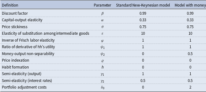
For the numerical exercises, two sets of parameters are calibrated.Footnote 4 The first column in Table 1 includes the values used for the standard model without money, while the second column presents the calibration of the model with money. The calibration for the New-Keynesian model is close to those used in Coibion and Gorodnichenko (Reference Coibion and Gorodnichenko>2011), while the model with money relies on the values estimated in Castelnuovo (Reference Castelnuovo>2012).
Model calibration

Notes: This table presents the calibration of the baseline New-Keynesian model with and without money. The shock parameters are all one-unit innovations.
3. Equilibrium determinacy under money aggregate targeting
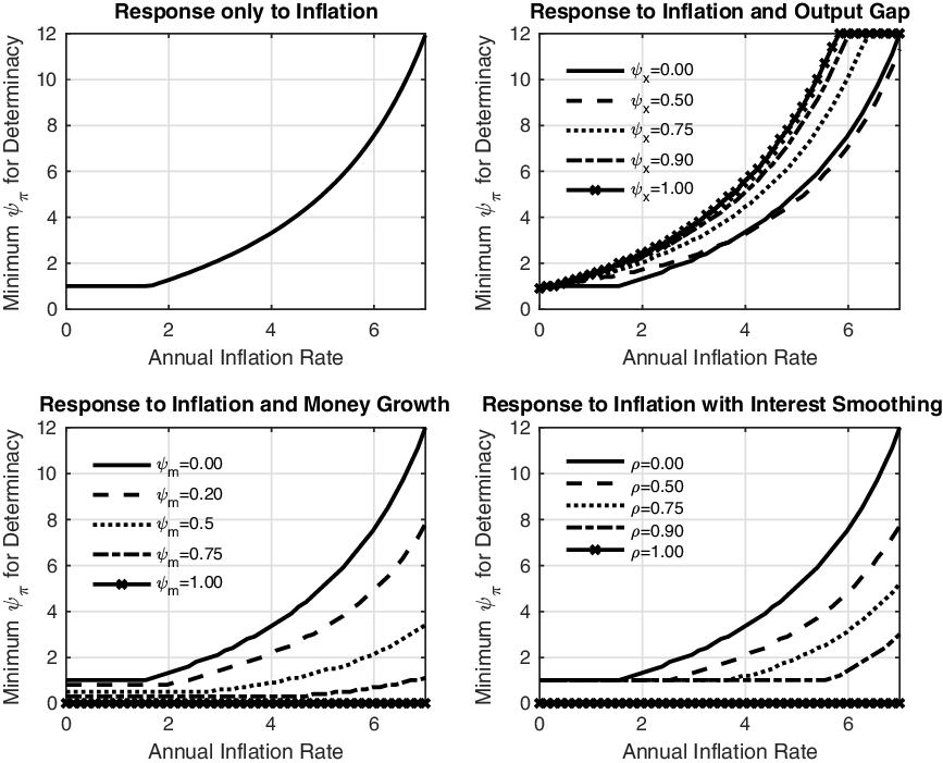
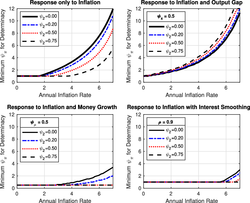
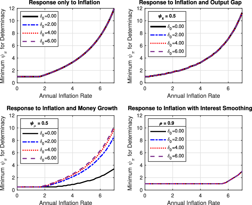
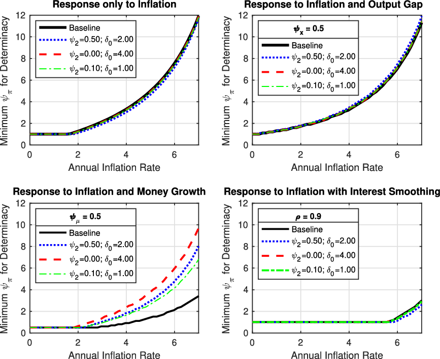
I illustrate the price-level determinacy properties of the monetary policy rule when the central bank responds to inflation, output, and growth in monetary aggregates. I focus on numerically evaluating determinacy under the following four model specifications with trend inflation but no money (Figure 1); trend inflation and non-separability between consumption and money (Figure 2); trend inflation and portfolio adjustment costs (Figure 3); trend inflation and the full model with money (Figure 4).
Determinacy under positive trend inflation (model without money).
Notes: This figure presents the minimum response of inflation (y-axis) required to ensure price determinacy regions under positive trend inflation (x-axis). Each response is conditional on various specifications of the feedback rule and the degree of non-separability, described in the plot title.

Determinacy under positive trend inflation and non-separability.
Notes: This figure presents the minimum response of inflation (y-axis) required to ensure price determinacy regions under positive trend inflation (x-axis). Each response is conditional on various specifications of the feedback rule and the degree of non-separability, described in the plot title.

Determinacy under positive trend inflation with portfolio adjustment costs.
Notes: This figure presents the minimum response of inflation (y-axis) required to ensure price determinacy regions under positive trend inflation (x-axis). Each response is conditional on various specifications of the feedback rule and the degree of non-separability, described in the plot title.

Determinacy under positive trend inflation (full model with money).
Notes: This figure presents the minimum response of inflation (y-axis) required to ensure price determinacy regions under positive trend inflation (x-axis). Each response is conditional on various specifications of the feedback rule and the degree of non-separability, described in the plot title.

3.1. Responding to inflation and output gap
To first connect with the benchmark literature, assume that the monetary authority only responds to inflation and the output gap. The familiar policy rule can be written as:
 \begin{equation} \hat{i}_{t} = \psi _{\pi } E_t\hat{\pi }_{t+j} + \psi _{x}E_t\hat{y}_{t+j} \end{equation}
As discussed in Woodford (Reference Woodford>2011), Galí (Reference Galí>2015), the special case of the contemporaneous version of the feedback rule (when
 $j = 0$
) satisfies the Taylor principle when
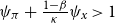 $\psi _{\pi } + \frac{1-\beta }{\kappa }\psi _{x} \gt 1$
, where
 $\kappa$
often represents the coefficient on the output gap in the standard NKPC. In the event of a sustained increase in the inflation rate of
 $\pi$
percent, the nominal interest rate will eventually be raised by more than
 $\pi$
percent, sufficing to determine an equilibrium price level. To eliminate the possibility of sunspot fluctuations, central banks must raise interest rates more than one-for-one with inflation. With
 $j= 1$
, as is the case considered in the following figures, an even stronger response is required to sustain determinate equilibria.
I focus first on how trend inflation alters the determinacy condition the Taylor rule loses its potency in environments with positive trend inflation, as emphasized in Hornstein and Wolman (Reference Hornstein and Wolman>2005), Kiley (Reference Kiley>2007), Ascari and Ropele (Reference Ascari and Ropele>2009), Coibion and Gorodnichenko (Reference Coibion and Gorodnichenko>2011). With the benchmark monetary policy rule, the minimum response needed by the central bank starts to rise, even for low levels of trend inflation. Intuitively, the breakdown of the basic Taylor principle is amplified due to the growing importance of forward-looking behavior in price-setting when trend inflation rises. A positive relationship emerges between the level of trend inflation and the minimum response to inflation required for a unique rational expectations equilibrium. The top panel of Figure 1 illustrates this result for the model with trend inflation but without money.
The top left panels of Figures 2, 3, and 4 highlight the impact of including features from the money portion of the model, such as with non-separability between consumption and real balances in the utility function (Figure 2), with portfolio adjustment costs (Figure 3), and with both combined (Figure 4). Figure 2 demonstrates that the reduction in the minimum response to inflation required for determinacy falls as the degree of non-separability rises under various levels of trend inflation. Simply put, the real balance effect makes even a one-for-one rise in both expected inflation and the nominal interest rate contractionary. This extra effect on aggregate demand is implied by the reduction in real money demand when an increase in the nominal interest rate occurs, exerting downward pressure on inflation and making price determinacy more likely. The rise in the nominal interest rate implied by the policy rule increases the opportunity cost of holding real money balances and, therefore, tends to reduce aggregate demand and inflation. It is also clear from the figure that these effects are even more pronounced when moving away from the zero trend inflation condition. This result extends the analysis of Kurozumi (Reference Kurozumi>2006) who shows that non-separability has implications for REE but only studies these features in a zero trend inflation case.
On the other hand, Figure 3 confirms that introducing portfolio adjustment costs does not affect the minimum response to inflation required to ensure the existence of a unique rational expectations inflation equilibrium. However, when non-separability is introduced back in the model, portfolio adjustment costs work to reduce the effect of non-separability in the money demand relationship. Combined (Figure 4), the introduction of portfolio adjustment costs counteract the effect of the non-separability between consumption and real balances as far as the minimum response to inflation for a REE is concerned.
I next focus on the case of a policy rule which includes a nonzero response to output (
 $\psi _{x} \neq 0$
) under positive trend inflation. In the model without money, the top right panel in Figure 1 simply replicates the findings of Kiley (Reference Kiley>2007), Ascari and Ropele (Reference Ascari and Ropele>2009), Coibion and Gorodnichenko (Reference Coibion and Gorodnichenko>2011), in that positive values of trend inflation require an even larger response to inflation to achieve determinacy since stronger responses to output gap can be destabilizing. This is because the slope of the NKPC turns negative for sufficiently high levels of trend inflation. Even small but positive responses to the output gap lead to a lower minimum response to inflation to achieve determinacy, but stronger responses have the reverse effect and necessitate a larger response to inflation to achieve price determinacy.
The top right panels of Figure 2 present the impact of non-separability between consumption and real balances in the utility function. The destabilizing effect of the output gap under positive trend inflation is sharpened as the degree of non-separability rises. Even a small degree of non-separability causes the Taylor rule to be much more likely to induce indeterminacy if this rule responds not only to inflation but also to output or the output gap. Once the extent of non-separability of the utility function surpasses a certain small threshold, the Taylor principle never implies its long-run version and it becomes a necessary condition. In this environment, a larger inflation coefficient than one, as implied by the Taylor principle, is required to sustain a determinate REE when responding to the output gap. This condition worsens under positive trend inflation. Figure 3 suggests that portfolio existence of adjustment costs does not affect the minimum response to inflation required for a determinate REE. As before, the combined effect of portfolio adjustment costs and non-separability negligibly raises the minimum response to inflation required for determinacy, given a fixed response to the output gap (
 $\psi _{x} = 0.5$
). The effects are noticeably sharper in a model with positive trend inflation.
Figure 3 augments this relationship by focusing only on portfolio adjustment costs and by setting non-separability to zero. As before, two separate mechanisms are at play when determining price-level determinacy: portfolio adjustment costs and trend inflation. While the degree of portfolio adjustment costs does not affect the response to inflation without non-separability in utility, a larger response to inflation is required for determinacy as trend inflation rises. Stronger responses to the output gap have the opposite effect and require an even larger response to inflation. Figure 4 further highlights this finding by varying the degree of portfolio adjustment costs. Once the extent of portfolio adjustment costs exceeds a certain small threshold, a larger inflation coefficient than what the Taylor principle suggests is required for determinacy.
3.2. Responding to inflation and money growth
To analyze price-level determinacy conditions when the monetary authority responds to inflation and money growth, the following policy rule is considered:
 \begin{equation} \hat{i}_{t} = \psi _{\pi } E_t\hat{\pi }_{t+j} + \psi _{\mu }E_t\hat{\mu }_{t+j} \end{equation}
Under this rule and with
 $j = 0$
, the condition
 $\psi _{\pi } + \psi _{\mu }\gt 1$
is sufficient to ensure the existence of a unique rational expectations inflation equilibrium in a zero trend inflation framework, as discussed in Keating and Smith (Reference Keating and Smith>2013). Responding sufficiently strongly to money growth (
 $ \psi _{\mu }\gt 1 - \psi _{\pi }$
) guarantees price determinacy even when the Taylor principle is not satisfied. With
 $j = 1$
as considered in the figures, an even stronger response to the policy coefficients is required to sustain determinate equilibria.
I generalize the properties of a policy rule with money to a model with positive trend inflation. The bottom left panel in Figure 1 suggests that the minimum level of inflation response needed for determinacy falls as the response to money growth rises. Responding to money and non-separability supplements the Taylor principle (
 $\psi _{\pi } \gt 1$
), which is not sufficient to establish a determinate REE with positive trend inflation. Figure 2 demonstrates that the effect of responding to money is stronger in the presence of non-separability of the utility function between consumption and real balances. Even lower response to inflation is required as the degree of non-separability rises for a fixed response to the money growth (
 $\psi _{\mu } = 0.5$
).Footnote 5
While the favorable properties of responding to money are still active, they become significantly weaker under portfolio adjustment costs. As shown in the bottom left panel of Figure 3, the minimum response to inflation rises as trend inflation rises even when the central bank responds moderately to money. It is also shown that larger portfolio adjustment costs raise the minimum response to inflation for a fixed response to money to achieve determinacy. The overall effect is shown in Figure 4, where, under the baseline calibration of the model with money, the net effect of both non-separability and portfolio adjustment costs raises the minimum response to inflation required for an REE, as compared to the case without both these effects. While in the baseline model without money, responding to money reduces the minimum response of the central bank to inflation, its overall effect with both non-separability and portfolio adjustment costs raises the minimum response for inflation required for a REE.
3.3. Interest rate smoothing
The last set of theoretical results analyze the case in which the monetary authority responds to money growth and partially smooths interest rates (with
 $\rho _{1}$
capturing the degree of smoothing in equation (18)).
 \begin{equation} \hat{i}_{t} = \rho _{1} \hat{i}_{t-1} + \psi _{\pi } E_t\hat{\pi }_{t+j} \end{equation}
The bottom right panel in Figures 1, 2, 3, and 4 plots the determinacy regions for the simple rule with a response to inflation and interest rate inertia under both zero and positive trend inflation with non-separability (Figure 2), portfolio adjustment costs (Figure 3), and the overall effects (Figure 4) when
 $j =1$
. As noted by Coibion and Gorodnichenko (Reference Coibion and Gorodnichenko>2011) and Woodford, (Reference Woodford>2001), higher interest rate smoothing makes determinacy sustainable at lower levels of the coefficient on inflation,
 $\psi _{\pi }$
. The result is consistent with the idea that history dependence is particularly useful in improving the determinacy properties of interest rate rules under trend inflation, aligning with the observations made in Arias et al., (Reference Arias, Ascari, Branzoli and Castelnuovo>2020). Interestingly, these properties extend to the case where there is non-separability in the utility function, between consumption and real balances, and portfolio adjustment costs. In Figure 4, I note that a larger degree of non-separability and portfolio adjustment costs assist with determinacy even at high values of trend inflation when the policy rule is inertial.
4. Money in federal reserve policy
4.1. Full-sample estimates
To test the role of money in formulating monetary policy, the baseline empirical specification for the Fed’s reaction function is a generalized Taylor rule, described in equations (14) and (15). The specification builds on Clarida et al.(Reference Clarida, Gali and Gertler>2000) and Taylor (Reference Taylor>1999) by including money in addition to a response to inflation and the output gap. I further use real-time data to estimate the policy rule. Because these data are (or were) available to the FOMC members at the time that policy decisions are (or were) made, a burgeoning literature has argued that these data are better able to gauge policy preferences compared to historical (or finally revised) data. My approach also relates to the literature that has tested for money in policy (Andrés et al. (Reference Andrés, López-Salido and Nelson>2009), Canova and Menz (Reference Canova and Menz>2011), Li et al. (Reference Li, Liu and Pei>2020), Castelnuovo (Reference Castelnuovo>2012). In contrast to this literature, I use Greenbook forecasts of current and future macroeconomic variables, prepared by staff members of the Fed before each FOMC meeting, to estimate this version of the policy rule. Finally, while the real-time data approach is in line with that used by Orphanides, (Reference Orphanides>2001, Reference Orphanides>2002, Reference Orphanides>2003), Boivin (Reference Boivin>2006), Coibion and Gorodnichenko (Reference Coibion and Gorodnichenko>2011), they do not allow money to play a role in the reaction function.
Data on money aggregate M1 are collected using the Greenbook from January 1969 to January 2002.Footnote 6 The other policy variables are matched with the real-time data as follows: the interest rate is the target federal funds rate set at each meeting, whereas the measures of the output gap and inflation are based on Greenbook forecasts, as also presented in Orphanides, (Reference Orphanides>2001, Reference Orphanides>2002, Reference Orphanides>2003)). I also estimate the policy rule where
 $\psi _{\mu }$
is set to 0 (or omitted from the regression specification), therefore, corresponding to a version estimated in Clarida et al. (Reference Clarida, Gali and Gertler>2000).
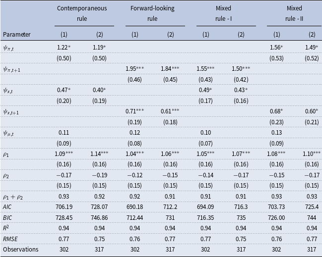
Table 2 summarizes the benchmark estimates of the policy rule using various combinations of the forecast horizon
 $j$
. Columns (1) of each version present the estimates of the full policy rule, while columns (2) present estimates of the simple Taylor rule (suppressing the coefficient on money to zero). While M1 enters with the right sign, it is not statistically significant. The coefficient on inflation varies across the forecast horizon considered with the best-fit version of the policy rule—determined by AIC/BIC tests as done in Coibion and Gorodnichenko (Reference Coibion and Gorodnichenko>2011)—suggest a strong long-run response to inflation and a high weight on the output gap.Footnote 7
Estimates of the policy rule (1969–2002)

Notes: This table presents OLS estimates of the baseline feedback rule. Standard errors are reported in parentheses.
 $^{*} p\lt 0.05$
,
 $^{**} p\lt 0.01$
,
 $^{***} p\lt 0.001$
denote significance levels. AIC and BIC denote the Akaike information criterion and Bayesian information criterion tests, respectively.
While the evidence presented in this section does not detect the role of money in an estimated version of the policy rule during the 1969–2002 period, the significance of this result may be contextualized based on the information available from the transcripts, and the analysis offered earlier: while money may have been important during the 1970s, its influence seems to have diminished during the 1980s. The full-sample approach ignores the important policy changes referred to in the literature purely because the fixed-coefficient approach does not highlight these changes. From an empirical perspective, (Clarida et al. (Reference Clarida, Gali and Gertler>2000), Boivin (Reference Boivin>2006), Coibion and Gorodnichenko (Reference Coibion and Gorodnichenko>2011)) provide evidence of important changes in the US conduct of monetary policy.
4.2. Split-sample estimates
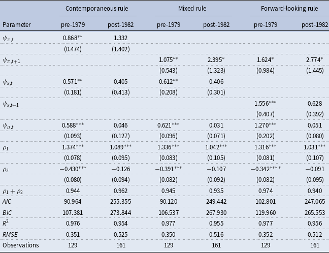
A standard single break in the coefficients of the response function around the time of the Volcker disinflation (October 1979) is allowed, following Coibion and Gorodnichenko (Reference Coibion and Gorodnichenko>2011). The policy rule is estimated for the period 1969 – October 1979 and the period 1982 – January 2002. Table 3 summarizes estimates of the policy rule using various combinations of the forecast horizon
 $j$
for each period.
Estimates of the policy rule (1969 – 1979 and 1982 – 2002)

Notes: This table presents OLS estimates of the baseline feedback rule. Standard errors are reported in parentheses.
 $^{*} p\lt 0.05$
,
 $^{**} p\lt 0.01$
,
 $^{***} p\lt 0.001$
denote significance levels. IV estimates can be shared upon request. AIC and BIC denote Akaike information criterion and Bayesian information criterion tests, respectively.
I find money to have exerted a statistically and economically significant impact on the federal funds rate during the pre-1979 sample, but not during the post-1982 sample. The best-fit version of the policy rule suggests a large response to money aggregate M1, during this period, with a value of 0.621. The systematic reaction of the Fed to money growth declines from a statistically significant value (0.621) to a statistically insignificant value of 0.031, signaling lower attention to monetary aggregate M1 in the second half of the sample. The coefficient on money is remarkably close to the estimates in Li et al. (Reference Li, Liu and Pei>2020), Castelnuovo (Reference Castelnuovo>2012), despite major differences in the data and estimation strategy.
Across the two time periods, other response coefficients seem to change as well. My estimates point to a stronger response, by the Fed, to inflation in the post-1982 period as compared to the pre-1979 period. Interest rate decisions become more persistent, in the sense that the sums of the autoregressive components are higher in the second period. Second, the Federal Reserve seems to have changed their response to the real side of the economy with a lower weight on the output gap in the second sample. This behavior of the policy coefficients is consistent with the estimates often found in the literature (Clarida et al. (Reference Clarida, Gali and Gertler>2000), Boivin (Reference Boivin>2006), and Coibion and Gorodnichenko (Reference Coibion and Gorodnichenko>2011). Standard AIC and BIC tests also confirm that, in terms of timing conventions, a mixed policy rule where the FOMC targeted forward-looking inflation but contemporaneous money and output gap best explains the setting of the federal funds rate.
An important result, concerning the pre-1979 estimates of the policy rule with money, suggests that including a response of the interest rate instrument to money growth affects the estimated coefficients of the other variables in the policy reaction function. Comparing the best-fit versions, (Coibion and Gorodnichenko (Reference Coibion and Gorodnichenko>2011)) estimate the weight on inflation to be 1.04 compared to 1.075 in this paper. They find that the weight on the output gap is equal to 0.52, whereas I find this to be equal to 0.612. Thus, the baseline Taylor rule coefficients are estimated to be quite close to the standard values found in the literature. The sum of the autoregressive coefficients is also estimated to be larger in Coibion and Gorodnichenko (Reference Coibion and Gorodnichenko>2011); the inclusion of money in the reaction function lowers these estimates in Table 2 as some of the inertia in policy actions seems to be explained by adding money growth in the policy rule. Across the estimated policy rules, the direction of bias is reversed for the post-1982 sample, as the coefficient on inflation is estimated to be higher in the model with money (2.395), as compared to a model without money (2.20), and the weight on the output gap is estimated to be lower (0.406), compared to 0.43.Footnote 8
The main results of this section suggest that M1 significantly influenced the policy rate during the pre-Volcker period, entering the reaction function positively. Moreover, the coefficient on money becomes statistically indistinguishable from zero during Volcker’s disinflation (from 1979 to 1982).Footnote 9 Including money also has the positive effect of improving the fit of the benchmark Taylor rule. By contrast, the policy rule without money appears to overestimate the coefficient on other variables, including inflation. It is important to mention that these findings extend a broad literature: on formalizing the role of money in FOMC policy as discussed in Sims and Zha (Reference Sims and Zha>2006), Li et al. (Reference Li, Liu and Pei>2020), Castelnuovo (Reference Castelnuovo>2012); and on presenting an alternative framework that better describes the monetary reaction function during the Great Inflation (Clarida et al. (Reference Clarida, Gali and Gertler>2000), Orphanides (Reference Orphanides>2001, Reference Orphanides>2002, Reference Orphanides>2003), Boivin (Reference Boivin>2006), Chowdhury and Schabert (Reference Chowdhury and Schabert>2008), Coibion and Gorodnichenko (Reference Coibion and Gorodnichenko>2011), Hirose et al. (Reference Hirose, Kurozumi and Van Zandweghe>2020)).
4.3. Applications to price determinacy
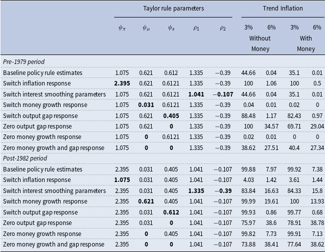
I combine the estimated policy parameters with the theoretical model described and calibrated in Section 2 to study price indeterminacy, both during the pre-1979 and the post-1982 period. I offer the results based on both the simple model without money but which includes a response to money growth and the full model with money, which includes all three channels through which money enters the model. I focus on using the best-fit version of the policy rule with money (“mixed policy rule,” as discussed in the previous section) for the split-sample policy coefficients offered in Table 3—the precise coefficients used in the Taylor rule, for the estimation, are also shared in the table. The analysis is conducted for two levels of trend inflation: 3% and 6%, designed to replicate average inflation rates in each of the two time periods. For each combination of the policy rule, I compute 10,000 draws to compute the fraction of determinate solutions for each level of trend inflation. For each draw, parameters of a Taylor rule are taken from the joint asymptotically normal distribution based on least squares estimates of Taylor rules. Coibion and Gorodnichenko (Reference Coibion and Gorodnichenko>2011) suggest that this procedure considers the estimation uncertainty associated with the systematic component of monetary policy. Table 4 reports these results.
Determinacy and counterfactual experiments

Notes: The table reports determinacy rates for the 1969–1979 (pre-1979) period and the 1982–2002 (post-1982) period for trend inflation rates of 3% and 6% with a model with and without money. Each row with “switch” contains the coefficient of the other period’s estimated rule, keeping the remaining policy parameters unchanged.
The baseline estimates (first row) suggest that the Fed’s response to inflation, in the pre-Volcker era, did not satisfy the Taylor principle for both levels of trend inflation. In particular, the pre-1979 response implies an indeterminate REE given the average inflation rate of that time (6%). This is a direct implication of the results presented in Section 2, as the Taylor principle weakens under high trend inflation. Notice, however, that the determinacy rates are almost always higher in the model without money (that is, without non-separability and portfolio adjustment costs but with a policy response to money). Notice that these results remain robust when I account for the complete transmission that allows money to play a more prominent role in shaping the macroeconomic dynamics.
Focusing on the baseline policy rule estimates for the post-1982 period, the change in the response to inflation and the reduction in trend inflation explain almost entirely the move from an indeterminate region to a determinate one. The post-1982 response is consistent with a determinate REE at the low average inflation rate of this period (3%). This result is robust to a model where money enters the structural mechanism (i.e. with non-separability and portfolio adjustment costs), even though money is not estimated to enter the policy rule in this period. The key result from this section suggests that allowing for monetarism, in the spirit of Sims and Zha (Reference Sims and Zha>2006), does not change the main conclusions offered in Clarida et al. (Reference Clarida, Gali and Gertler>2000)) and (Coibion and Gorodnichenko (Reference Coibion and Gorodnichenko>2011)) in that the shift from indeterminacy to determinacy appears to have taken place, going from the pre-1979 period to the post-1982 sample.
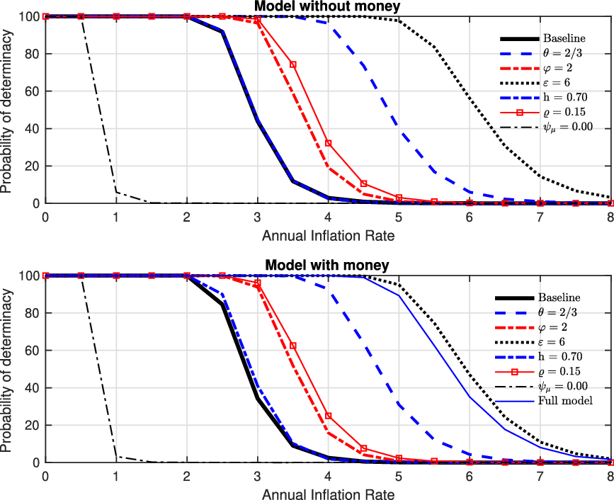
Likelihood of a determinate REE: Robustness (Pre-1979).
Notes: The figure summarizes the benchmark results and robustness of results on determinacy using alternative assumptions on price-setting (
 $\theta$
), elasticity of substitution (
 $\varepsilon$
), Frisch elasticity of labor supply (
 $\varphi$
), indexation (
 $\varrho$
), and habit formation (
 $h$
) in the model with (
 $\psi _\mu \neq 0$
) and without (
 $\psi _\mu = 0$
) money. I compute 10,000 draws to compute the fraction of cases (scaled to be between 0 and 100) with determinate solutions for each combination of trend inflation. For each draw, parameters of a Taylor rule are taken from the joint asymptotically normal distribution based on least squares estimates of Taylor rules. Additional robustness checks are offered in Qureshi (Reference Qureshi>2018).

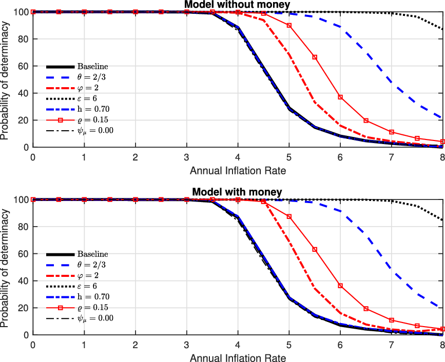
Likelihood of a determinate REE: Robustness (Post-1982).
Notes: The figure summarizes the benchmark results and robustness of results on determinacy using alternative assumptions on price-setting (
 $\theta$
), elasticity of substitution (
 $\varepsilon$
), Frisch elasticity of labor supply (
 $\varphi$
), indexation (
 $\varrho$
), and habit formation (
 $h$
) in the model with (
 $\psi _\mu \neq 0$
) and without (
 $\psi _\mu = 0$
) money. I compute 10,000 draws to compute the fraction of cases (scaled to be between 0 and 100) with determinate solutions for each combination of trend inflation. For each draw, parameters of a Taylor rule are taken from the joint asymptotically normal distribution based on least squares estimates of Taylor rules.

4.4. Counterfactual experiments
I offer counterfactual experiments that determine the contribution of each of the policy changes and the trend inflation to the likelihood of determinacy in each regime. For instance, I generate determinacy rates by switching the pre-1979 response to inflation with the post-1982 response as shared in the “switch inflation response” row. The counterfactual exercise suggests that if this specific policy was in place, REE determinacy would be guaranteed for both model specifications at 3% trend inflation but not at 6% trend inflation. Similarly, switching the interest rate response does not change the baseline results. Switching the money growth response to the post-1982 level (or setting it to zero) replicates the findings of Coibion and Gorodnichenko (Reference Coibion and Gorodnichenko>2011), as the percentage of draws that suggest determinacy falls to levels close to 0% for the pre-1979 period for both 3% and 6% trend inflation. A key implication of this result is that while responding to money raises the likelihood of determinacy at 3% trend inflation, it is not sufficient to counteract the higher trend inflation observed during this time period. The likelihood of a determinate REE is even lower in the model with money.
Switching the pre-1979 response to output gap with the post-1982 response generates determinacy for both models at 3% trend inflation but not at 6% trend inflation. However, draws for determinacy are higher in a model where money does not play a role. While responding to money increases the likelihood of determinacy compared to the estimated in Coibion and Gorodnichenko (Reference Coibion and Gorodnichenko>2011), it is not large enough to counteract the effect of high trend inflation both with and without money in the model. This sharpens the point made by Orphanides (Reference Orphanides>2004), who emphasizes the consequence of the decline in response to the output gap over the two periods. In the second regime, from 1982 to 2002, the strong response to inflation is sufficient to rule out price indeterminacy, a finding in line with the classic explanation of the Great Moderation offered by Clarida et al. (Reference Clarida, Gali and Gertler>2000) and Coibion and Gorodnichenko (Reference Coibion and Gorodnichenko>2011) and others. However, this result depends on the level of trend inflation in the model. The likelihood of determinacy under 6% inflation is low and below 10%. This is consistent with the conclusions reached by Coibion and Gorodnichenko (Reference Coibion and Gorodnichenko>2011): if the Fed in the 1970s had simply switched to the current policy rule without simultaneously engaging in the Volcker disinflation, it is quite possible that the US economy would have remained subject to self-fulfilling expectations-driven fluctuations. This is true even when the high response to inflation is combined with the large response to money growth estimates for the pre-1979 period.
4.5. Sensitivity analysis
Several parameters related to the structural mechanism could influence these results. Greater price stickiness increases the sensitivity to expectations of future macroeconomic variables, thereby, influencing the percentage of draws that point to indeterminacy. Non-separability and portfolio adjustment costs could also influence the quantitative results. These effects are further sharpened as the degree of habit formation rises. Figure 5 summarizes the benchmark results and the counterfactual percentage of determinacy draws based on alternative assumptions related to the structural parameters and the various levels of trend inflation consistent with the pre-1979 period. Figure 6 presents this exercise for the post-1982 period.
With higher Frisch elasticity of labor supply, the percentage of draws that point to determinacy rises but remains well below the 50% threshold. The inclusion of habit formation and mild values of indexation does not change these results. For latter, it is important to note that indexation diminishes the determinacy issues that arise with positive trend inflation because it decreases the devaluation of the firms’ re-set prices that comes from positive trend inflation. As noted earlier, in the special case with full indexation or
 $\varrho = 1$
, determinacy in the model is unaffected by the level of trend inflation in the model. However, Ascari et al. (Reference Ascari, Castelnuovo and Rossi>2011) note that a low level of indexation is consistent in models with trend inflation. In the model, I use their estimated range of values for indexation (which lie below 0.30) to show that the key results do not change at this estimated value.
I set the degree of price stickiness used in Galí (Reference Galí>2015), which is between the value proposed by Bils and Klenow (Reference Bils and Klenow>2004) and the upper bound of the value proposed by Nakamura and Steinsson (Reference Nakamura and Steinsson>2008), and consistent with a pricing change of every 11 months. The likelihood of determinacy rises, as expected, but remains well below 20%. In the model with money, the likelihood is close to 0% for the alternative pricing assumptions at 6% trend inflation.
A lower elasticity of substitution,
 $\varepsilon$
, also affects determinacy outcomes in both models. Setting a lower value of
 $\varepsilon = 6$
, which implies markups of 20%, is observed to empirically raise the likelihood of determinacy. Interestingly, in the model without money, the likelihood is close to 50%, raising concerns about the robustness of the results when the (Coibion and Gorodnichenko (Reference Coibion and Gorodnichenko>2011)) framework of analysis is combined with a response to money. However, the likelihood of determinacy falls well below 40% in the model when money is allowed to play an active role (through non-separability and portfolio adjustment costs).Footnote 10 Figure 6 confirms the baseline results presented earlier, in that determinacy in the post-1982 period is achieved given the low level of trend inflation observed during this period and the switch to a more active policy. This result is robust for all calibrations of the model, both when money plays a role and when it does not. The post-1982 response converges with the conclusions offered by Coibion and Gorodnichenko (Reference Coibion and Gorodnichenko>2011) and detects a determinate REE at the low average inflation rate of this period (3%).
5. Conclusion
I develop a business cycle model with positive trend inflation where money is allowed to play a role through non-separability between consumption and real balances, portfolio adjustment costs, and an explicit response by the central bank to money growth. I show that the Taylor principle changes in this environment. Targeting money enables the central bank to be sufficiently active, guaranteeing REE for even high levels of trend inflation. I show that this outcome is sensitive to the inclusion of non-separability between consumption and real balances and portfolio adjustment costs. In other words, the model with money behaves very differently as far as a determinate REE is concerned when moving away from the zero trend inflation assumption.
I apply this framework to analyze the rise in macroeconomic instability experienced by the US economy during the 1970s. I use briefing forecasts, prepared for the Federal Open Market Committee (FOMC), to estimate a policy rule with money for the 1969–2002 time period. Along with inflation and the output gap, money aggregate M1 exerted a statistically and economically significant impact on policy behavior. The exclusion of money aggregates from the policy rule seems to be an important source of bias in the previous estimations of the reaction function and has important consequences for the role of monetary policy during the Great Inflation.
The evidence suggests that the response to money was, perhaps, not sufficiently strong to complement the relatively weak response to inflation and counteract the high trend inflation of the pre-Volcker period, especially in the model with money. The overall findings generally support the conclusions of Clarida et al. (Reference Clarida, Gali and Gertler>2000) and Coibion and Gorodnichenko (Reference Coibion and Gorodnichenko>2011), but do so in a framework that specifically accounts for a role for money.
A. Appendix
A.1. Optimality conditions
In Section 2, the representative household maximizes its expected utility (1) subject to its budget constraint (equation (2)) over the following choice variables consumption (
 $C_{t}$
), labor hours (
 $N_{t}$
), real money holdings (
 $M_{t}/P_{t}$
), and bonds (
 $B_{t}$
), yielding the following optimality conditions:
 \begin{equation} \lambda _{t} = \beta E_{t} \frac{i_{t}\lambda _{t+1}}{\Pi _{t+1}} \end{equation}
 \begin{equation} a_{t} N^{\varphi }_{t} = \lambda _{t}\frac{W_{t}}{P_{t}} \end{equation}
 \begin{equation} \lambda _{t} = a_{t}\frac{\Psi _{1,t}}{C^h_{t-1}} - h\beta E_{t}\left [\left (\frac{C_{t+1}}{C^{h+1}_{t}}\right )a_{t+1}\Psi _{1,t+1} \right ] \end{equation}
 \begin{equation} \lambda _{t} = \frac{a_{t}}{e_{t}}\Psi _{2,t}- \frac{\partial G(m_{t}, m_{t-1})}{\partial m_{t}} - \beta E_t\frac{\partial G(m_{t+1}, m_{t})}{\partial m_{t}}+ \beta E_{t} \left [\frac{\lambda _{t+1}}{\Pi _{t+1}} \right ] \end{equation}
In equations (A.1)–(A.4),
 $\lambda _{t}$
denotes the Lagrange multiplier,
 $m_{t} = \frac{M_{t}}{P_{t}}$
are the real balances, and
 $\Pi _{t+1} = \frac{P_{t+1}}{P_{t}}$
is the (gross) rate of inflation. The terms
 $\Psi _{1,t}$
and
 $\Psi _{2,t}$
are the partial derivatives of the utility function with respect to the first and second choice variables. The symbols
 $\frac{\partial G(m_{t}, m_{t-1})}{\partial m_{t}}$
and
 $\frac{\partial G(m_{t+1}, m_{t})}{\partial m_{t}}$
stand for the partial derivatives of the portfolio adjustment cost function
 $G (\!\bullet \!)$
with respect to
 $m_{t}$
, evaluated at
 $t$
and
 $t+1$
, respectively. These are written as:
 \begin{equation} \frac{\partial G(m_{t}, m_{t-1})}{\partial m_{t}} = \frac{d}{2}\left \{ \exp \!\left [c\left (\frac{m_t}{m_{t-1}}-1\right )\right ]\left (\frac{c}{m_{t-1}}\right ) + \exp \!\left [-c\left (\frac{m_t}{m_{t-1}}-1\right )\right ]\left (-\frac{c}{m_{t-1}}\right ) \right \} \end{equation}
 \begin{equation} \frac{\partial G(m_{t+1}, m_{t})}{\partial m_{t}} = \frac{d}{2}\left \{ \exp \!\left [c\left (\frac{m_{t+1}}{m_{t}}-1\right )\right ]\left (-\frac{c m_{t+1}}{m^2_{t}}\right ) + \exp \!\left [-c\left (\frac{m_{t+1}}{m_{t}}-1\right )\right ]\left (-\frac{c m_{t+1}}{m^2_{t}}\right ) \right \} \end{equation}
The first-order condition of the firms’ problem can be derived by maximizing equation (4) subject to equation (5) and can be written as:
 \begin{equation} \bigg (\frac{P^{\ast}_{i,t}}{P_{t}}\bigg )^{1+\frac{\varepsilon \alpha }{1-\alpha }} = \frac{\varepsilon }{(\varepsilon -1)(1-\alpha )}\frac{E_{t}\!\sum _{j = 0}^{\infty } \theta ^{j}D_{t,t+j} \frac{W_{t+j}}{P_{t+j}} \bigg (\frac{Y_{i,t}}{z_{t}}\bigg )^{\frac{1}{1-\alpha }} \bigg [\frac{\Pi ^{\varrho }_{t-j,t+j-1}}{\Pi _{t,t+j}} \bigg ] ^{\frac{-\varepsilon }{1-\alpha }}}{E_{t}\!\sum _{j = 0}^{\infty } \theta ^{j}D_{t,t+j}\bigg [\frac{\Pi ^{\varrho }_{t-j,t+j-1}}{\Pi _{t,t+j}} \bigg ] ^{1-\varepsilon }Y_{i,t+j}} \end{equation}
Note that future expected inflation rates enter both the numerator and the denominator and, thus, affect the relative weight on future variables. With positive trend inflation, two effects come into play. When intermediate firms are free to adjust, they will set higher prices to try to offset the erosion of relative prices and profits that trend inflation automatically creates. Second, expectation of forward-looking terms is progressively multiplied by larger discount factors. This means that optimal price-setting under trend inflation reflects future economic conditions more than the short-run cyclical variations. Price-setting firms become more forward-looking. Price indexation mitigates these two effects. Setting
 $P_{t} = \bigg [\int _{0}^{1} P_{i,t}^{1-\varepsilon } di \bigg ]^{\frac{1}{1- \varepsilon } }$
, and
 $\bigg (\frac{P^{\ast}_{i,t}}{P_{t}}\bigg ) = p^{\ast}_{i,t}$
, enables me to write the pricing equation as:
 \begin{equation} 1 = \theta \pi ^{(1-\varepsilon )\varrho }_{t} + (1-\theta )(p^{\ast}_{i,t})^{(1-\varepsilon )} \end{equation}
Notice that equation (A.7) can be written in a recursive formulation of the optimal price-setting equation:
 \begin{equation} (p^{\ast}_{i,t})^{1+\frac{\varepsilon \alpha }{1-\alpha }} = \frac{\varepsilon }{(\varepsilon -1)(1-\alpha )}\frac{\psi _{t}}{\phi _{t}} \end{equation}
To simplify this expression, I define the auxiliary variables as recursive formulations:
 \begin{equation} \psi _{t} = w_{t}Y^{\frac{1}{1-\alpha }}_{t}z^{\frac{-1}{1-\alpha }}_{t}\lambda _{t} + \theta \beta \pi ^{\frac{-\varrho \varepsilon }{1-\alpha }}_{t} E_{t}\bigg [\pi ^{\frac{\varepsilon }{1-\alpha }}_{t+1}\psi _{t+1} \bigg ] \end{equation}
 \begin{equation} \phi _{t} = Y_{t}\lambda _{t} + \theta \beta \pi ^{{\varrho }{(1-\varepsilon )}}_{t}E_{t}\bigg [\pi ^{\varepsilon -1}_{t+1}\phi _{t+1}\bigg ] \end{equation}
Moving onto the labor market, the expression for the intermediate inputs (
 $Y_{i,t}$
) is first combined to find an expression for the aggregate labor demand:
 \begin{equation} N^d_{t} = \int _{0}^{1} N^d_{i,t}di = \int _{0}^{1} \bigg (\frac{P_{i,t}}{P_{t}}\bigg )^\frac{-\varepsilon }{1-\alpha } di \bigg (\frac{Y_{t}}{z_{t}}\bigg )^\frac{1}{1-\alpha } = s_{t}\bigg (\frac{Y_{t}}{z_{t}}\bigg )^\frac{1}{1-\alpha } \end{equation}
which is equation (7) in the main text. Finally, Ascari et al. (Reference Ascari, Castelnuovo and Rossi>2011) show price dispersion to evolve as:
 \begin{equation} s_{t} = (1-\theta )(p^{\ast}_{i,t})^\frac{-\varepsilon }{(1-\alpha )} + \theta \pi _{t-1}^\frac{-\varepsilon \varrho }{1-\alpha } \pi _{t}^\frac{\varepsilon }{1-\alpha }s_{t-1} \end{equation}
A.2. The steady-state
Before log-linearizing the model, I find the steady-state terms by imposing the following restrictions on the first-order conditions:
 $C_{t} = Y_{t}$
,
 $a_{t} = a_{t+1} = \bar{a}$
,
 $e_{t} = e_{t+1} = \bar{e}$
,
 $z_{t} = z_{t+1} = \bar{z}$
,
 $N_{t} = \bar{N}$
,
 $\lambda _{t} = \lambda _{t+1} = \bar{\lambda }$
,
 $C_{t-1} = C_{t} = C_{t+1} = \bar{y}$
,
 $m_{t-1} = m_{t} = m_{t+1} = \bar{m}$
,
 $w_{t} = \bar{w}$
,
 $\Pi _{t+1} = \Pi _{t} = \bar{\Pi }$
,
 $\psi _{t} = \psi _{t+1} = \bar{\psi }$
,
 $\phi _{t} = \phi _{t+1} = \bar{\phi }$
,
 $s_{t-1} = s_{t} = \bar{s}$
,
 $MC_{t} = \bar{MC}$
,
 $p^{\ast}_{i,t} = \bar{p}^{\ast}_{i}$
. It is important to note that the steady-state inflation
 $\bar{\Pi }$
affects all key relationships in the model.
 \begin{equation} \bar{\Pi } = \beta \bar{r} \end{equation}
 \begin{equation} \bar{w} \bar{\lambda } = \bar{a}\bar{N}^{\varphi } \end{equation}
 \begin{equation} \bar{\lambda } \bar{y}^h = (1-\beta h) \bar{a} \bar{\Psi }_{1} \end{equation}
 \begin{equation} \bar{e} \bar{\lambda } (\bar{\Pi } - \beta) = \bar{a} \bar{\Pi }\bar{\Psi }_{2} \end{equation}
 \begin{equation} \bar{MC} = \frac{1}{1-\alpha } w \left ( \frac{\bar{y}^\alpha }{\bar{z}} \right )^\frac{1}{1-\alpha } \end{equation}
 \begin{equation} \bar{N} = \bar{s} \left ( \frac{\bar{y}}{\bar{z}} \right )^\frac{1}{1-\alpha } \end{equation}
 \begin{equation} \bar{s} = \frac{1-\theta }{1-\theta \bar{\Pi }^\frac{\varepsilon (1-\varrho )}{1-\alpha }}(p^{\ast}_{i})^\frac{-\varepsilon }{1-\alpha } \end{equation}
 \begin{equation} \bar{\psi } = \frac{\bar{w}\bar{\lambda }\!\left ( \frac{\bar{y}}{\bar{z}} \right )^\frac{1}{1-\alpha }}{1-\theta \beta \bar{\Pi }^{\frac{\varepsilon (1-\varrho )}{1-\alpha }}} \end{equation}
 \begin{equation} \bar{\phi } = \frac{\bar{y}\bar{\lambda }}{1-\theta \beta \bar{\Pi }^{(\varepsilon -1)(1-\varrho )}} \end{equation}
 \begin{equation} (\bar{p}^{\ast}_{i})^{1+\frac{\varepsilon \alpha }{1-\alpha }} = \frac{\varepsilon }{(\varepsilon -1)(1-\alpha )}\frac{\bar{\psi }}{\bar{\phi }} \end{equation}
 \begin{equation} (\bar{p}^{\ast}_{i}) = \left [\frac{1-\theta \bar{\Pi }^{(\varepsilon -1)(1-\varrho )}}{1-\theta }\right ]^{\frac{1}{1-\varepsilon }} \end{equation}
 \begin{equation} y(\bar{\Pi }) = \left (\frac{(1-\alpha )(1-\beta h)}{ \bar{s}^{\varphi }} \bar{z}^{\frac{\varphi +1}{1-\alpha }} \Psi _{1} \bar{MC} \right )^{\frac{1-\alpha }{\varphi -h +\alpha (1+h)}} \end{equation}
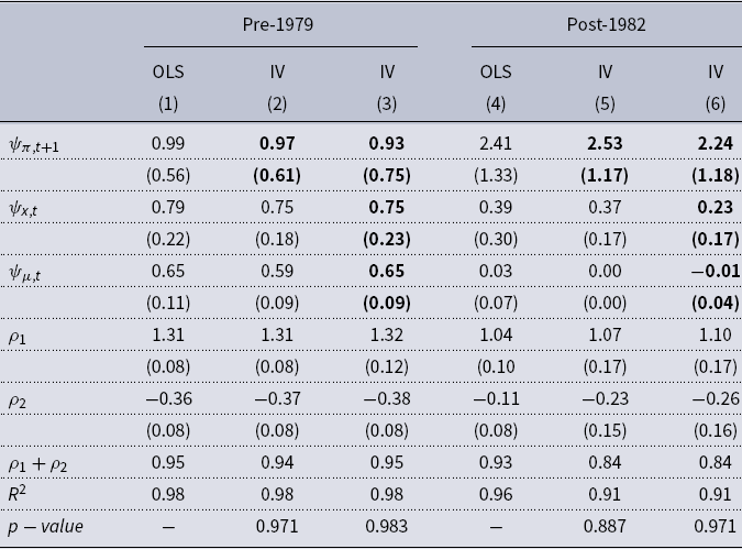
A.3. IV estimates of the split-sample policy rule
The following table (Table 5) presents the least squares and instrumental variable estimates of the benchmark (mixed) Taylor rule with money. Following Coibion and Gorodnichenko (Reference Coibion and Gorodnichenko>2011), I use the past values of inflation, money growth, and output gap from the Greenbook.
Estimates of the policy rule—OLS and IV estimates

This table presents the OLS and IV estimates of the baseline feedback rule. Standard errors are reported in parentheses. The set of instruments are lags of inflation, output gap, the federal funds rate, and growth in monetary aggregate M1. The bold letters are the instrumented variables. The bottom panel reports the p-value associated with a test of the over-identifying restrictions (Hausman).
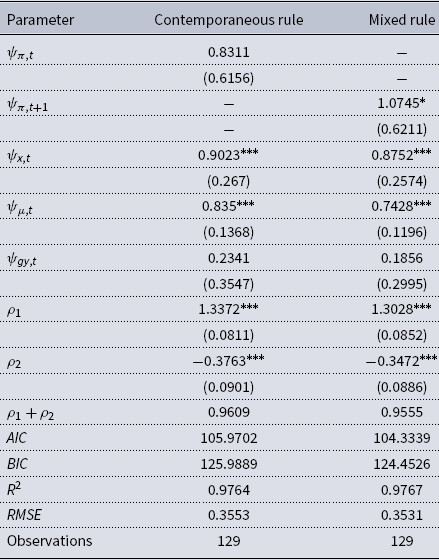
A.4. Comparison between money growth and output growth in the policy rule
Estimates of the policy rule (1969–1979): money growth vs. output growth

Notes: This table presents the OLS estimates of the baseline feedback rule. Standard errors are reported in parentheses.
 $^{*} p\lt 0.05$
,
 $^{**} p\lt 0.01$
,
 $^{***} p\lt 0.001$
denote significance levels. AIC and BIC denote the Akaike information criterion and Bayesian information criterion tests, respectively.