1. Introduction
Vascular interventional devices can be categorized into two main types: stationary devices and mobile devices. The former includes medical stents, artificial valves, and particles [Reference Vaziri, Zirak, Azadi, Keshmiri and Shokri1–Reference Gul, Tzirtzilakis and Makhanov6], while the latter comprises catheters, guidewires, and interventional robots [Reference Alapan, Bozuyuk, Erkoc, Karacakol and Sitti7–Reference Liu, Zhang, Du, Zhang, He, Li and Song11]. Among these, vascular interventional robots are capable of autonomous movement within blood vessels. Hemodynamics – encompassing blood velocity, pressure, and wall shear stress (WSS) – is fundamental to vascular diagnosis and treatment.
Owing to the periodic ejection of blood by the heart, blood flow exhibits a pulsatile nature. Meanwhile, blood vessels possess elastic and distensible properties, leading to fluid-structure interaction (FSI) between flowing blood and deformed vessels. Many computational hemodynamics studies have simplified the vessel wall as rigid to reduce computational cost. However, for large elastic arteries such as the carotid artery – the target vessel in this study – wall compliance significantly influences both flow dynamics and vessel mechanics. Rigid-wall models inherently neglect wall motion, leading to substantial errors in predicted hemodynamic parameters.
Albadawi et al. compared rigid-wall and elastic-wall models in both carotid and coronary stenotic arteries, demonstrating that the assumption of wall rigidity systematically alters WSS and blood velocity distributions, particularly in post-stenotic regions where flow recirculation occurs [Reference Albadawi, Abuouf, Elsagheer, Sekiguchi, Ookawara and Ahmed12]. In a more quantitative study of symptomatic stenosed carotid arteries, Jodko et al. reported that the difference between compliant-wall and rigid-wall models exceeded 35% for peak-systolic area-averaged WSS and reached 42% and 43% for time-averaged local vorticity and shear strain, respectively [Reference Jodko, Jeckowski and Tyfa13]. Such large discrepancies underscore the necessity of FSI for accurate hemodynamic assessment in large arteries.
Malvè et al. studied unsteady blood flow in a left coronary artery bifurcation using both CFD (rigid wall) and FSI (compliant wall). Their results revealed not only remarkable qualitative differences in WSS patterns but also relevant quantitative differences under transient flow conditions, further confirming that rigid-wall models cannot capture the protective effect of wall compliance [Reference Malvè, García, Ohayon and Martínez14]. Torii et al. performed a patient-specific FSI analysis of the right coronary artery with physiological waveforms, showing that increased systolic pressure dilates the vessel and consequently lowers WSS – a phenomenon completely absent in rigid-wall simulations [Reference Torii, Wood, Hadjiloizou, Dowsey, Wright, Hughes, Davies, Francis, Mayet, Yang, Thom and Xu15]. In an experimental study using particle image velocimetry (PIV) on rigid versus compliant models of healthy carotid arteries, Geoghegan et al. found that rigid boundaries cause a severe overestimation of WSS, with the maximum relative difference reaching up to 60% compared to the compliant model [Reference Geoghegan, Jermy and Nobes16]. Collectively, these studies demonstrate that rigid-wall models overestimate WSS by 35–61% and fail to capture wall motion-induced flow modifications, making FSI essential for reliable hemodynamic quantification in the carotid artery.
When an interventional device is present, the vessel’s internal structure changes, further altering flow and deformation. Badal et al. analyzed three stent designs in coronary arteries using FSI, suggesting that polylactic acid (PLA) may reduce restenosis risk [Reference Badal, Mohapatra, Bhoi, Sharma, Jena and Panda17]. Ghosh et al. employed FSI to investigate polymer-based surgical aortic valve replacement [Reference Ghosh, Marom, Rotman, Slepian, Prabhakar, Horner and Bluestein18]. Stahl et al. applied FSI to study an intracranial tumor shunt [Reference Stahl, Marsh, Thormann, Ding, Saalfeld, Behme and Berg19]. Wang et al. simulated guidewire insertion into a Y-shaped coronary artery [Reference Wang, Fu and Fei20]. However, all these FSI studies focus on stationary devices or passively moved guidewires. In contrast, a vascular interventional robot actively moves within the bloodstream and typically features a spiral surface structure for plaque removal and vascular dredging. To address this gap, we previously incorporated FSI to analyze hemodynamic parameters during robot intervention [Reference Zhu, Ji, Liang, Wang, Xia and Tang21]. When a robot is present, hemodynamic changes are jointly influenced by the vessel, the blood, and the robot itself. For a specific individual, vessel and blood properties are relatively constant, whereas the robot’s spiral structural parameters – spiral pitch, groove depth, and thread profile – must be designed in advance to ensure safety and efficacy.
A critical question thus arises: how do variations in these spiral parameters affect hemodynamic parameters and vessel wall displacement? From the perspective of this research, wall displacement is particularly important. The robot either contacts the vessel wall or moves in close proximity. Excessive wall displacement may indicate mechanical overstress and risk of vascular injury (e.g., dissection or aneurysm formation), while insufficient displacement could imply inadequate robot–wall interaction for effective plaque removal. Only an FSI model can simultaneously compute wall displacement and its coupling with blood flow, thereby providing a direct assessment of the safety risk of vessel over-expansion or collapse. Rigid-wall models, by definition, cannot provide any information on wall motion and would completely ignore this safety-critical aspect. Moreover, the magnitude and statistical significance of the influence of each spiral parameter on both flow parameters and wall displacement require in-depth investigation. Answering these questions is essential for designing safe vascular interventional robots.
This paper references the diameter and blood flow characteristics of the carotid artery, incorporates the elastic properties of blood vessels, and systematically analyzes the effects of spiral structural parameters of vascular interventional robots on both hemodynamic parameters and vascular wall displacement. Furthermore, it identifies the primary, secondary, and statistically significant influences of each spiral parameter, thereby providing a rational basis for designing the spiral structure of vascular interventional robots.
2. Vascular interventional robot system
In Figure 1, the vascular interventional robot system comprises four core components: blood vessels, blood, a magnetic vascular robot, and an external magnetic driving device. The robot features a capsule-like structure, with its outer shell integrated with a spiral design. Both the internal magnet (housed within the capsule) and the external permanent magnet adopt a radial magnetization configuration. To drive the robot, a mechanical arm and a motor are employed to control the external magnet – enabling it to perform translational and rotational movements, which in turn prompts the robot to execute corresponding motions inside the blood vessel.
Schematic diagram of a vascular interventional robot system.

3. Numerical calculation method
3.1. Theoretical equations
It is assumed that the blood fluid is unaffected by temperature and exhibits incompressible properties. The governing equations for the fluid domain (blood) are as follows [Reference Han, Ren, Lian, Luo, Liu, Ma, Li, Deng and Liu22]:
 \begin{equation} \nabla \cdot \boldsymbol{v}_{f}=0 \end{equation}
 \begin{equation} \rho _{f}\frac{\partial \boldsymbol{v}_{f}}{\partial t}+\rho _{f}((\boldsymbol{v}_{f}-\boldsymbol{v}_{b})\cdot \nabla)\boldsymbol{v}_{f}=\nabla \cdot \boldsymbol{\tau }_{f} \end{equation}
The governing equation for the solid domain (blood vessel) is expressed as follows:
 \begin{equation} \nabla \cdot \boldsymbol{\tau }_{s}=\rho _{s}\overset{..}{\boldsymbol{d}_{s}} \end{equation}
where Hamiltonian operator
 $\nabla =\boldsymbol{i}\frac{\partial }{\partial x}+\boldsymbol{j}\frac{\partial }{\partial y}+\boldsymbol{k}\frac{\partial }{\partial z}$
,
v
f
is the fluid velocity vector, ρ
f
is the fluid density, t is time,
v
b
is the velocity vector of the moving boundary,
τ
f
is the fluid stress tensor,
τ
s
is the solid stress tensor, ρ
s
is the solid density, and
 $\overset{..}{\boldsymbol{d}_{s}}$
is the local acceleration of the solid domain.
Owing to the FSI between the fluid and solid domains, their interface must satisfy the following conditions:
 \begin{align} \begin{cases} \boldsymbol{d}_{f}=\boldsymbol{d}_{s}\\ \boldsymbol{\tau }_{f}\cdot \boldsymbol{n}=\boldsymbol{\tau }_{s}\cdot \boldsymbol{n} \end{cases} \end{align}
where d f and d s are the displacement vectors of the fluid and the solid, respectively, and n is the boundary normal vector.
It is assumed that the interventional robot moves horizontally along the central axis of the blood vessel and rotates around its own central axis. The position equation for any point on the robot’s surface is:
 \begin{align} \begin{cases} x(t)=x_{0}+v_{r}t\\[3pt] y\left(t\right)=y_{0}+r\cos \dfrac{\pi n_{r}}{30}t\\[8pt] z\left(t\right)=z_{0}+r\sin \dfrac{\pi n_{r}}{30}t \end{cases} \end{align}
where t is time, (x(t), y(t), and z(t)) are the position coordinates of the point at time t, x 0, y 0, and z 0 are the initial position coordinates of the point, r is the distance from the point to the robot’s central axis, v r is the translational speed of the robot, and n r is the rotational speed of the robot with a unit of r/min.
3.2. Model and parameters
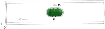
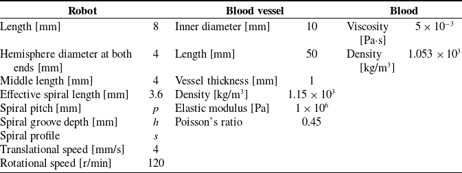
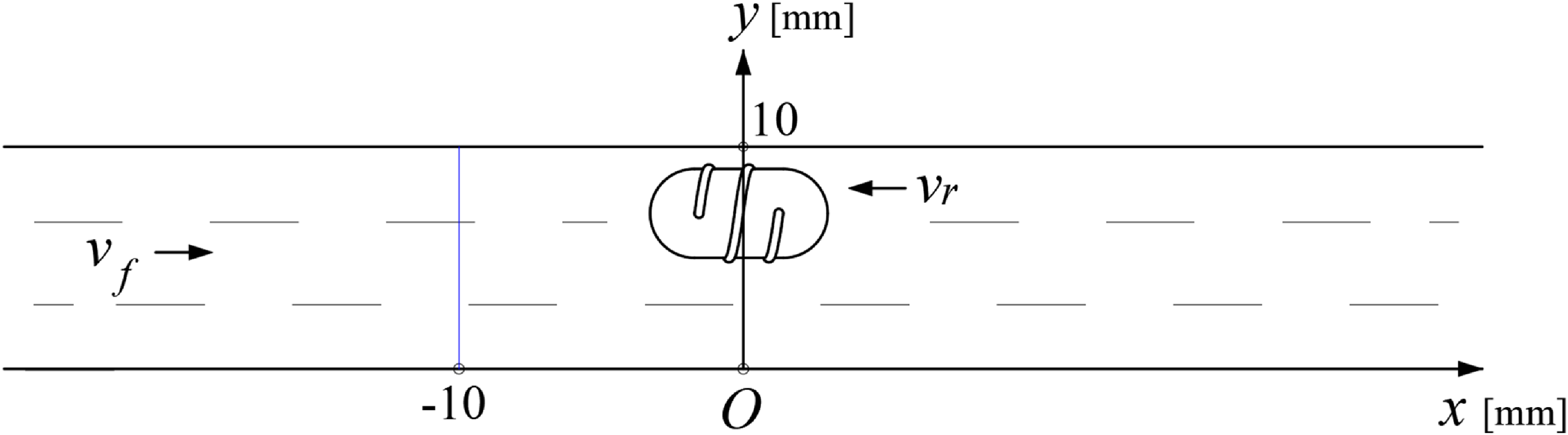
The 3D computational model, illustrated in Figure 2, comprises a blood vessel, blood, and an interventional robot. To simplify the calculations, blood is treated as a Newtonian fluid, and the blood vessel is assumed to be a linear elastic material when the interventional robot is rotating and translating at high speed. It is assumed that the robot is introduced at a location distal to the heart and advances toward the heart; notably, the direction of blood flow is opposite to the robot’s movement direction. Both the blood flow and the robot’s motion are aligned along the x-axis, denoted by v f (blood flow velocity) and v r (robot translational velocity), respectively. For the fluid flow field calculation, to accurately simulate the robot’s translational and rotational movements, a layer of “wrapping fluid” is defined on the surface of the interventional robot.
Computational model of a vascular interventional robot system.

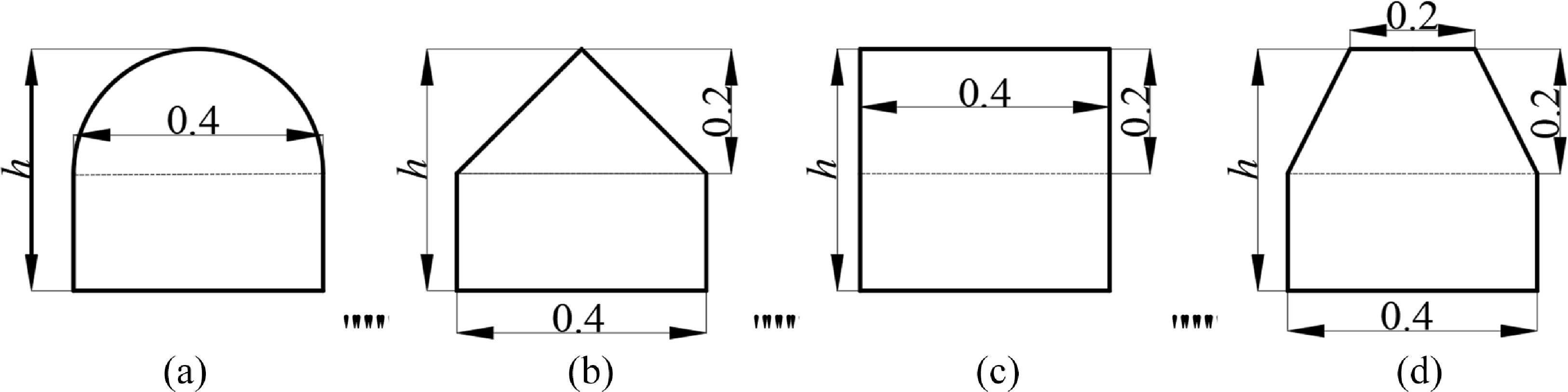
The spiral parameters of the vascular robot include spiral pitch (p), spiral groove depth (h), and spiral profile (s). To facilitate comparison, in Figure 3, the upper half of the spiral profile adopts four different shapes – semicircle, isosceles triangle, rectangle, and isosceles trapezoid – while the lower half is uniformly designed as a rectangle with its height increasing from 0. The relevant parameters of the computational model are presented in Table 1.
Spiral profile and groove depth. (a) Semicircle. (b) Triangle. (c) Rectangle. (d) Trapezoid.

Relevant parameters of the computational model

3.3. Mesh analysis
The meshes in the blood (fluid) domain are composed of tetrahedral and wedge-shaped elements. In contrast, the meshes in the vascular (structural) domain are hexahedral. Fluid mesh inflation layers are applied at the interfaces between the blood and vessel regions, as well as at the interfaces between the blood region and the robot surface. The two inflation layers are both configured with 5 sub-layers and a growth ratio of 1.2. The generated mesh is shown in Figure 4.
Generated mesh. (a) Overall view of the fluid domain. (b) Enlarged view of the inflation layer in the fluid domain. (c) Structural domain.

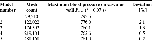
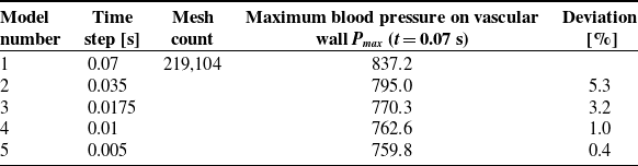
Maximum blood pressure on the vascular wall, Pmax (t = 0.07 s), is selected as the evaluation indicator for conducting mesh independence analysis and time step convergence verification. On the premise that mesh quality meets computational standards, Tables 2 and 3 show how Pmax alters with varying mesh quantities and time step sizes. The results show that Pmax tends to stabilize once the mesh count increases to 219,104. Furthermore, with a fixed mesh number of 219,104 and a time step of 0.01 s, Pmax maintains nearly constant values.
3.4. Boundary conditions
According to ref [Reference Kumar, Pai, Abdul Khader, Khan and Kyriacou23], the measured blood velocity data of the carotid artery were fitted using the 7th-order Fourier series Eq. (6), and the corresponding fitting curve is presented in Figure 5. The coefficients (a 0, a n , and b n ) listed in Table 4 were derived from the waveform that best matched the measured curve.
The curve in Figure 5 was adopted as the inlet boundary condition for the computational model. For computational convenience and consistency with some previous studies, a zero-pressure boundary condition was applied at the outlet. Additionally, the inlet and outlet end faces of the blood vessel were configured as fixed supports with zero displacement.
 \begin{equation} v_{\mathrm{inlet}}\left(t\right)=\mathit{a}_{0}+{\sum }_{n=1}^{N}\left(a_{n}\cos \left(n\omega t\right)+b_{n}\sin \left(n\omega t\right)\right) \end{equation}
3.5. FSI method and solution settings
The robot’s motion influences blood flow, while the blood flow in turn induces vascular deformation – this deformation further affects blood flow, resulting in a FSI phenomenon. The flowchart of the FSI method is presented in Figure 6. During the FSI calculation process, the fluid domain (i.e., blood) and the structural domain (i.e., the solid blood vessel) are solved in parallel. Specifically, blood flow and robot motion jointly drive changes in the fluid flow field; the fluid domain then transmits pressure data to the structural domain, which subsequently generates boundary displacements for the structural domain. These displacements cause deformation of the computational domain, and the structural domain further feeds back position and velocity data to the fluid domain. This iterative process persists until the calculation cycle is completed. The entire numerical calculation was performed using Ansys® software.
The translational speed of the robot (v r ) is set to 4 mm/s, which is implemented via a user-defined function (UDF). For the robot’s rotational motion, its rotational speed (n r ) is 120 r/min, achieved using the sliding mesh method. Notably, the rotational speed of the wrapping fluid is consistent with that of the robot. Since the robot’s rotation induces a turbulent state of the fluid within the vessel, the standard k-ε turbulence model is selected for simulation. For this model, the turbulence intensity (I) is set to 5%, and the hydraulic diameter (D) is specified as 10 mm. To solve the coupled equations of fluid pressure and velocity, the standard SIMPLE algorithm is adopted. Additionally, a second-order upwind scheme is chosen for the difference format of all parameters to ensure calculation accuracy. The residual convergence criterion is set to 0.001 for the continuity equation, velocity components in the x, y, and z directions, as well as the k and ε variables. All field variables in the fluid domain are initialized to zero.
A transient calculation mode is adopted, with the time step set to 0.01 s for fluid, solid, and FSI modules, and the total calculation time is 0.8 s. The system coupling surface is defined as the interface between the fluid domain and the structural domain, enabling accurate data transmission between the two domains.
Mesh independence analysis

Time independence verification

Inlet velocity curve.

Fluid domain mesh deformation is mainly caused by two factors: the prescribed rigid translational motion of the robot and the large flexible deformation of the structural boundary induced by fluid–structure interaction. To maintain mesh quality throughout the numerical simulation and avoid excessive distortion of computational cells, a combined dynamic mesh strategy is adopted in our study. Firstly, a mesh smoothing algorithm based on the diffusion equation is applied to smoothly propagate the displacement of the wall boundary into the fluid domain and realize the orderly update of internal mesh node positions. Meanwhile, a mesh quality threshold is predefined, and local mesh remeshing is automatically triggered when the mesh skewness exceeds 0.85. This dynamic mesh scheme can dynamically update the fluid computational mesh following the real-time motion of the solid boundary, which effectively suppresses mesh distortion and avoids negative volume. It maintains satisfactory mesh quality during the entire transient fluid–structure interaction calculation, thereby ensuring the numerical accuracy and computational stability of the simulation.
4. Experimental verification
To verify the correctness and feasibility of the aforementioned numerical method, a pulsatile fluid measurement system for magnetically controlled microrobots in pipes was constructed [Reference Zhu, Ji, Liang, Wang, Xia and Tang21], as illustrated in Figure 7.
Coefficient values of the Fourier series equation

Flowchart of the FSI method.

The experimental system consists of two core modules: a magnetic actuation module for microrobot manipulation and a PIV module for measuring pulsatile fluid flow fields. The experimental pipe is fabricated from transparent elastic plastic, and the experimental fluid is transparent methyl silicone oil. Notably, the elastic modulus of the pipe approximates that of human arteries. The viscosity of the experimental fluid is also close to that of human whole blood. These design choices ensure the biological relevance of the experiment. The microrobot’s shell is precision-machined from black bioplastic. Key parameters of the pipe, fluid, and microrobot are summarized in Table 1. Specifically, the microrobot shell adopts a semicircular spiral profile with a pitch of 1.75 mm and a spiral groove depth of 0.25 mm. The internal magnet of the microrobot is a solid cylinder with a diameter of 2 mm and a length of 2 mm. For microrobot actuation, an external permanent magnet is driven by a robotic arm and a rotary motor. It can realize three-axis translational motion and rotational motion around the central axis of the microrobot. The external permanent magnet is designed as a hollow cylindrical structure with an inner diameter of 18 mm, an outer diameter of 35 mm, and a length of 20 mm. Both the external and internal magnets are made of N38-grade neodymium-iron–boron (NdFeB) material. Its maximum magnetic energy product is 310 kJ/m3, the residual magnetic flux density is 12.5 kGs, and the coercivity is 899 kA/m. The distance between the central axes of the two magnets is fixed at 29 mm. The experimental moving speed of the microrobot is consistent with the setting adopted in numerical calculations. This arrangement guarantees good comparability between experimental and simulated results. A complete coordinate system is established as shown in Figure 8. In terms of flow field data collection, all measured data are collected at the moment when the inlet velocity of the pipe reaches the state corresponding to point B in Figure 5.
Pulsatile fluid measurement system for magnetically controlled microrobots. (a) Global view. (b) Local view. (c) Semicircular spiral microrobot.

Orientation and coordinate system of the microrobot in the artery model.

Figure 9 compares the x-component of the fluid velocity at two positions (x = −10 mm and x = 0 mm) illustrated in Figure 8 during the robot’s precession, with the experimental values representing the average of multiple measurements. At the position far from the robot, as the pipe is traversed from top to bottom, the fluid velocity first increases, then stabilizes, and finally decreases. This trend is consistent with the velocity distribution of fluid flow inside a circular pipe. In contrast, at the position where the robot is located, the fluid velocity first increases, then decreases rapidly, and eventually drops to zero when traversing the pipe from top to bottom. For both positions, the numerical simulation results and experimental measurements exhibit good agreement in terms of both variation trends and magnitude. The relatively larger discrepancy between the calculated and measured results in Figure 9(b) can be attributed to two factors: first, the fluid flow surrounding the robot is significantly more turbulent, leading to greater complexity in flow behavior; second, the numerical model assumes the robot moves steadily along the horizontal x-axis throughout the simulation, whereas minor vertical (up-and-down) fluctuations of the robot were observed during the experiment. As evident from Figure 9(a) and (b), the intervention of the robot increases the fluid velocity in its vicinity. Collectively, these findings validate the correctness and feasibility of the numerical method employed in this study.
Calculated and measured results. (a) x = −10 mm. (b) x = 0 mm.

5. Spiral structure design and analysis
The orthogonal method is an efficient experimental design approach for investigating multi-factor, multi-level systems. By analyzing the results of orthogonal tests, one can gain insights into the overall performance of comprehensive experiments and, ultimately, obtain optimal test outcomes with the minimum number of trials. Figure 10 illustrates the optimization design process proposed in this study, which integrates the FSI calculation method with the orthogonal design method.
Block diagram of the optimization design method.

When the interventional robot operates within a blood vessel, the key hemodynamic and vascular parameters include the maximum blood velocity (vmax ), maximum blood pressure (Pmax ), maximum vascular wall shear stress (τmax ), and maximum vascular deformation (fmax ). Based on the magnitudes of these parameters, an orthogonal numerical calculation approach was employed to investigate the influence degree, significance, and optimal combination of the robot’s structural parameters.
5.1. Orthogonal numerical calculation
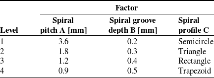
As presented in Figures 2 and 3, the factors selected for the orthogonal design include spiral pitch (p), spiral groove depth (h), and spiral profile (s), which are respectively labeled as Factors A, B, and C. Each factor is set with four levels, and the level values of each factor are uniformly selected under the reasonable operating conditions of the robot; these levels are arranged to form the L16(43) orthogonal table [Reference Fang and Ma24]. The specific settings of the three factors and their corresponding four levels are presented in Table 5.
Factors and levels

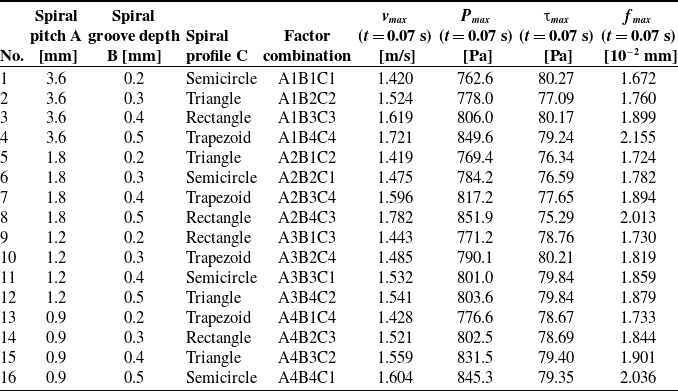
Calculating all 64 (43) combinations of structural parameters would result in an excessively large computational load. Therefore, 16 representative schemes, as listed in Table 6, were selected. Numerical calculations were then performed for all 16 sets of structural parameters to obtain the corresponding hemodynamic and vascular parameters.
Orthogonal calculation results

5.2. Range analysis
The range R reflects the relative degree of influence of each factor on the calculated target parameters. A larger value of R indicates a more significant impact of changes in the factor’s levels on the target parameters [Reference Tang, Liang, Guo, Liu and Hu25].
Range calculation results

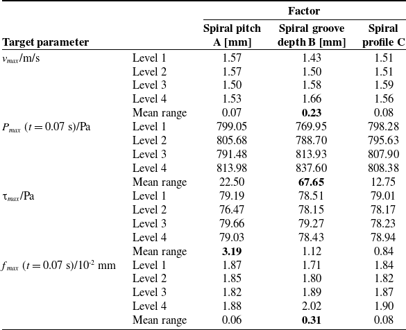
Table 7 shows the mean range of different target parameter values under different factors. The results indicate that the spiral pitch, spiral groove depth, and spiral profile of the robot surface exert varying degrees of influence on the four target parameters. Specifically, the relative influence magnitudes of each factor on the parameters are as follows:
-
For blood velocity: spiral groove depth
 $\gt$
spiral profile ≈ spiral pitch;
-
For blood pressure: spiral groove depth
$\gt$
spiral pitch > spiral profile; -
For vascular wall shear stress: spiral pitch
$\gt$
spiral groove depth
$\gt$
spiral profile; -
For vascular deformation: spiral groove depth
$\gt$
spiral profile ≈ spiral pitch.


It can be concluded that variations in the spiral structural parameters of the vascular robot have differential effects on the hemodynamic and vascular parameters. Among these factors, spiral groove depth exerts a more significant influence on most target parameters and thus serves as the primary factor; in contrast, spiral profile has a relatively weaker influence across the parameters and is therefore classified as the secondary factor.
5.3. Variance analysis
Range analysis enables the determination of the priority order regarding the importance of influencing factors. However, to objectively assess the significance of each factor’s impact on the calculated target parameters, further variance analysis is required [Reference Fang and Ma24].
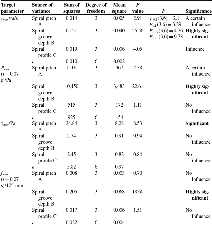
Table 8 presents the variance analysis results of the effects of robotic spiral parameters on hemodynamic and vascular parameters. Its F value serves as the core test statistic for the variance analysis of orthogonal experiments. Essentially, they represent the ratio of variation caused by each factor to the variation of random errors and are used to quantitatively evaluate the significance of the influence of each factor on the experimental indexes. A larger F value indicates a more significant effect of the corresponding factor on the experimental index and a lower probability that the result is caused by accidental random errors; conversely, a smaller F value means the influence is closer to random errors with weaker significance. The significance level can be further classified, and the hypothesis test can be completed according to the theoretical critical value and degrees of freedom of the F distribution.
Variance analysis

Regarding blood velocity, the influence of spiral groove depth is highly significant, while the other two factors (spiral pitch and spiral profile) also exert a measurable influence.
For blood pressure, spiral groove depth has a highly significant influence, spiral pitch has a certain degree of influence, and spiral profile has almost no influence.
In terms of vascular wall shear stress, the influence of spiral pitch is significant, whereas spiral groove depth and spiral profile have nearly no impact.
For vascular deformation, spiral groove depth exhibits a highly significant influence, while the other two factors have almost no influence.
These results confirm that among the spiral structural parameters, spiral groove depth is the most critical influencing factor – it exerts a highly significant effect on blood velocity, blood pressure, and vascular deformation. Additionally, spiral pitch only has a significant influence on vascular wall shear stress, while spiral profile is deemed an insignificant factor across all hemodynamic and vascular parameters analyzed.
5.4. Parameter selection of the spiral structure
The structural parameters of the vascular microrobot are regarded as reasonable only when the hemodynamic indicators and vascular deformation remain within the physiological normal range of the human body, which avoids abnormal blood flow, over-limit flow velocity, abnormal vascular deformation, and vascular rupture. Specifically, the level of each influencing factor is determined to ensure optimal target performance parameters.
For the vascular robot to perform safe diagnosis and treatment inside blood vessels, its associated hemodynamic and vascular parameters must be controlled within a reasonable range. Specifically, blood velocity, blood pressure, and vascular wall shear stress should be maintained at moderate levels, while vascular deformation should be kept relatively minimal. As indicated in Tables 5 and 6, blood velocity, blood pressure, and vascular deformation are primarily determined by the robot’s spiral groove depth, and all exhibit a proportional relationship with this target parameter; in contrast, vascular wall shear stress is mainly governed by the robot’s spiral pitch. Therefore, to ensure blood velocity and blood pressure remain within the reasonable range, the robot’s spiral groove depth should be minimized as much as possible to reduce vascular deformation. Simultaneously, an appropriate spiral pitch should be selected to maintain vascular wall shear stress at a moderate level. Additionally, the robot’s spiral profile can be reasonably adjusted based on the diagnostic and therapeutic requirements for different blood vessels. When a thrombus is present in a blood vessel and the vascular robot is required to perform dredging, the spiral robot should employ a triangular profile, a smaller groove depth, and a moderately sized pitch.
5.5. Effects of robotic device and wall boundary conditions on hemodynamics
Table 9 compares the hemodynamic parameters at peak systole (t = 0.07 s) under three different conditions. The results show that the presence of the robotic device significantly alters the flow field characteristics. The maximum velocity v max in the cases with the robot (1.420 m/s and 1.341 m/s) is higher than that in the case without the robot (1.275 m/s). More notably, under the FSI condition considering blood and vessel interaction, the maximum pressure P max and wall shear stress τ max with the robotic intervention (762.6 Pa and 80.27 Pa) are substantially higher than those in the case without the robot, indicating that the robot introduces a significant disturbance to the local hemodynamics.
Hemodynamic parameters at peak systole (t = 0.07 s) for three different simulation cases

Comparing the two cases with robotic intervention, it is found that all hemodynamic parameters obtained under the FSI assumption are higher than those under the rigid wall assumption: v max increases from 1.341 m/s to 1.420 m/s, P max increases from 697 Pa to 762.6 Pa, and τ max increases from 48.36 Pa to 80.27 Pa. In addition, the wall displacement f max is non-zero in the FSI cases, reaching 1.672 × 10⁻² mm in the Robot + FSI case, while it is zero in the rigid wall case. These results indicate that the rigid wall assumption underestimates the actual flow-induced loads and vascular responses, and the FSI model is necessary to capture realistic vessel deformation and its effects on the hemodynamic environment.
6. Conclusions
6.1. Study limitations
Our study simplifies blood by adopting the Newtonian fluid assumption, while real blood is a non-Newtonian fluid. The hyperelastic deformation characteristics and bifurcated structure of real blood vessels are neglected; blood vessels are simplified into linearly elastic walls and straight pipes with constant diameter for calculation. The particle effect of blood cells is ignored, and blood is regarded as a single-phase continuous fluid.
In this paper, the Unsteady Reynolds-Averaged Navier–Stokes (URANS) method combined with the standard k−ε turbulence model is adopted to solve the flow field. It should be noted that the standard k−ε model has inherent limitations in the simulation of the near-wall region. This model usually relies on wall functions to handle the viscous sublayer and buffer layer, making it difficult to accurately characterize the velocity gradient and wall shear stress distribution within the near-wall boundary layer. In the problem of blood-vessel interaction, the near-wall effect exerts a crucial influence on flow characteristics and the force acting on blood cells. Therefore, the current model is limited in accuracy when dealing with such flows. Subsequent research may consider adopting the SST k−ω turbulence model, which can perform direct integration down to the wall in the near-wall region and is expected to improve the simulation accuracy of the boundary layer.
In addition, the URANS method can essentially only resolve large-scale unsteady flow structures, while small-scale turbulent eddies are processed by temporal averaging via the turbulence model. It cannot fully reproduce the multi-scale turbulent characteristics around the robot, which may lead to certain errors in the simulation results of local flow details and wall shear stress.
6.2. Conclusions and future work
Active vascular interventional robots often adopt surface spiral structures to dredge stenotic blood vessels. In this study, considering FSI, the fluid flow field around a moving spiral micro-robot in an elastic pipe under pulsatile flow conditions was investigated through both theoretical and experimental approaches. The results show that the variation trends and numerical magnitudes of the calculated and measured data are basically consistent. Furthermore, using the range and variance analysis methods in orthogonal design, the influence laws of the spiral parameters of the robot’s surface structure on the hemodynamic and vascular parameters were explored. It is found that spiral groove depth is the primary factor affecting hemodynamic and vascular parameters – it exerts a highly significant influence on blood velocity, blood pressure, and vascular deformation. Spiral pitch, as a secondary factor, has a highly significant impact on vascular wall shear stress; in contrast, spiral profile has a negligible influence on hemodynamic parameters. To achieve the goal of non-invasive interventional diagnosis and treatment using the vascular robot, the robot should be designed with a smaller spiral groove depth, a moderate spiral pitch, and a spiral profile with stronger cutting capability. In conclusion, the FSI method, PIV technique, and orthogonal design method can be widely applied to the parameter calculation, measurement, and optimization of mobile interventional devices operating in elastic blood vessels filled with pulsatile blood. Future work should focus on the complex physiological environments of blood and blood vessels, including the multiphase flow model of blood, as well as the hyperelastic characteristics and complex geometries of blood vessels.
Author contributions
Yu Liu and Liang Liang conceived the study, designed the methodology, and conducted the theoretical analysis and numerical simulations. Weiming Zhou and Xiangping Duan completed the experimental setup, data acquisition, and data curation. Yu Liu performed the data processing, result analysis, and manuscript drafting. Liang Liang supervised the entire research and revised the manuscript critically for important intellectual content. All authors have read and approved the final version of the manuscript for submission.
Financial support
This work was supported in part by the National Natural Science Foundation of China under grant 52575198, the Natural Science Foundation of Hunan Province under grant 2026JJ80036, and the Open Project of Hunan Provincial Engineering Research Center under grant 2023KFKT11.
Conflicts of interest
The authors declare no conflicts of interest exist.
Ethical approval
Not applicable.
Use of AI
Doubao AI (Doubao-Seed-2.0, ByteDance Inc.), accessible at https://www.doubao.com, was used for English polishing and grammar revision of this manuscript on 31 May 2026. No proprietary information was disclosed, and no tool modifications or additional datasets were introduced by the authors. No competing interests or potential biases arise from the use of this AI tool.