Implications
Due to costs, breeding programs tend to genotype more animals with low-density panels and obtain the remaining genotypes through imputation from a higher density panel. With a reasonable sized reference population, high imputation accuracies are often obtained. Although imputation accuracy seems to decay only slightly per generation even in absence of updating of the reference population, that was not the case for GEBVs. However, a modest updating of the reference population will reduce substantially the decay in the reliability of GEBVs and provides a viable and cost effective alternative for implementation of genomic selection.
Introduction
Advances in DNA sequencing technology and the increased availability of high-density single nucleotide polymorphism (SNP) genotyping platforms provided unprecedented opportunities to enhance breeding programs in livestock, poultry and plant species and to better understand the genetic basis of complex traits. Using this genomic information in a breeding program within the so called genomic selection (GS) requires dense marker maps covering the whole genome to track effectively all potential QTLs affecting the trait through linkage disequilibrium (LD) with genotyped SNP markers (Meuwissen et al., Reference Meuwissen, Hayes and Goddard2001). In several applications it seems that 50K SNPs provides a reasonable coverage. In livestock and poultry, major advances have been realized in the last few years, and GS is becoming a routine technique, mainly due to the decreasing costs of genotyping for high-density SNP marker panels.
However, high accuracies are achieved only when a reasonable number of SNPs are genotyped for each individual. Unfortunately, the current cost precludes their extensive use in some livestock and poultry applications. For example, selection of replacement heifers in dairy and beef herds would be too expensive to be conducted using high-density SNP panels and low-density SNP chips (e.g. 3K or 7K) may be the only cost effective option available (Pryce and Hayes, Reference Pryce and Hayes2012). Therefore, low-density and low-cost SNP marker chips could represent a practical viable alternative that would reduce the genotyping costs. However, to use low-density panels in genomic breeding values (GEBVs) estimation, the non-genotyped SNP markers need to be inferred. This could be accomplished using imputation techniques to predict the non-genotyped SNPs resulting, thus, in a denser coverage. Genotype imputation, a cost effective in-silico genotyping of non-genotyped SNP markers, allows breeders to genotype animals with affordable low-density panels and predict the un-typed genotypes from the high-density panel (Weigel et al., Reference Weigel, Van Tassell, O’Connell, VanRaden and Wiggans2009; Druet et al., Reference Druet, Schrooten and de Roos2010; Zhang and Druet, Reference Zhang and Druet2010; VanRaden et al., Reference VanRaden, O’Connell, Wiggans and Weigel2011).
Based on the genomic information used to derive the missing genotypes, imputation methods could be divided into two categories: (1) pedigree-based imputation, and (2) population-based imputation. Pedigree-based imputation uses the correlation of genotypes among relatives derived from the sharing of genomic segments identical by descent within pedigrees and linkage information. In contrast, population-based imputation leverages information from the correlation among dense markers due to LD. Several imputation software are already available including fastPHASE (Scheet and Stephens, Reference Scheet and Stephens2006), MaCH (Li et al., Reference Li, Willer, Ding, Scheet and Abecasis2010), Beagle (Browning and Browning, Reference Browning and Browning2007) and IMPUTE2 (Howie et al., Reference Howie, Donnelly and Marchini2009), which were designed specifically for human populations, using only LD information. AlphaImpute (Hickey et al., Reference Hickey, Kinghorn, Tier, van der Werf and Cleveland2012), FImpute (Sargolzaei et al., Reference Sargolzaei, Chesnais and Schenkel2011) and findhap (VanRaden et al., Reference VanRaden, O’Connell, Wiggans and Weigel2011), which were developed for animal and plant applications, use pedigree and linkage information. It is worth mentioning that FImpute has an option to impute missing genotypes based on population and/or pedigree information. Accuracy of genotype imputation is influenced by several factors; including the number and distribution of markers on the low-density panel, the number of individuals genotyped using the high-density chip (reference population) and their genetic relationships with the animals to be imputed, allele frequencies at the SNP markers and the local LD between each low-density genotype and its surrounding high-density genotypes (Zhang and Druet, Reference Zhang and Druet2010; Huang et al., Reference Huang, Xu, Xie, Zhou and Qu2011; Hickey et al., Reference Hickey, Kinghorn, Tier, van der Werf and Cleveland2012). Several studies (Badke et al., Reference Badke, Bates, Ernst, Fix and Steibel2014; Chen et al., Reference Chen, Li, Sargolzaei and Schenkel2014; Sargolzaei et al., Reference Sargolzaei and Schenkel2014) have already been conducted to evaluate the efficiency of SNP genotype imputation under different conditions with special emphasis on the accuracy of imputed genotypes and their impact on the quality of the genomic predictions. However, little attention has been paid to the imputation accuracy and its potential impact on GS after several cycles of selection.
Several analytical approaches have been proposed for genome-based prediction of genetic values. The main difference stems from the assumptions about the marker effects (Meuwissen et al., Reference Meuwissen, Hayes and Goddard2001; de los Campos et al., Reference de los Campos, Gianola and Rosa2009; Habier et al., Reference Habier, Fernando, Kizilkaya and Garrick2011). GS is currently implemented either through multiple regression or variance component-based models. Although these methods have different statistical and biological assumptions regarding the data generating process, they tend to yield similar results in most cases and the differences are largely due to the genetic architecture of the trait, the genetic relationships between individuals in the sample, and the chosen prior information. With the inclusion of imputed SNP genotypes, it is reasonable to assume that the accuracy of GEBV will depend on the error rate of the imputation in addition to the method used to estimate marker effects (Luan et al., Reference Luan, Woolliams, Lien, Kent, Svendsen and Meuwissen2009), the heritability of the trait (Calus and Veerkamp, Reference Calus and Veerkamp2007), the population structure (Hayes et al., Reference Hayes, Bowman, Chamberlain and Goddard2009; Habier et al., Reference Habier, Tetens, Seefried, Lichtner and Thaller2010) and the size of the reference population (VanRaden et al., Reference VanRaden, Null, Sargolzaei, Wiggans, Tooker, Cole, Sonstegard, Connor, Winters, van Kaam, Valentini, Van Doormaal, Faust and Doak2009). Furthermore, the impact of genotype imputation errors could be different between the different methods used in GS.
The aim of this study is: (1) to investigate the decay of imputation accuracy over time (generations) under several simulation scenarios; and (2) to evaluate the impact of multi-generational SNP genotype imputation on the accuracy of GEBV obtained using either regression or variance-based methods.
Material and methods
Simulation
Population structure
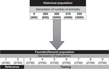
Genomic data were simulated using QMSim software (Sargolzaei and Schenkel, Reference Sargolzaei, Chesnais and Schenkel2009) and consisted of 42 000 SNP markers and 1500 QTLs distributed across 30 chromosomes. Simulating genomic data via QMSim software consists of a two-step process as indicated in Figure 1. In the first step, a historical population is generated. In our case, a population of 600 individuals was maintained through random mating for 200 generations followed by an additional 205, 210 and 220 generations with population size of 5000, 4000 and 3000, respectively, in order to create initial LD and establish mutation-drift equilibrium in the historical generations. The sex ratio in the historical generations was maintained and the mating system was based on random union of gametes, randomly sampled from both the male and female gamete pools.
A schematic representation of the layout of the simulated data structure.

In the second step of the simulation, the founder population is generated and labelled as generation 0 (G0). In our case, this population was generated from the last historical generation, based on 300 males and 2700 females. The mating of these individuals was at random and no selection was considered at this step. Then after the recent population, nine generations were simulated and later used to evaluate the imputation process.
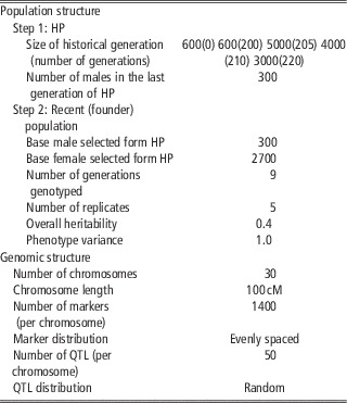
For the most recent generations, it was assumed one progeny per dam per year, a sex ratio of 50% in the progeny; selection was based on EBV with a replacement rate of 50% for sires and 20% for dams. Selected sires and dams were randomly mated. A single trait with an overall heritability of 0.40 and phenotypic variance of 1.0 was simulated. The true breeding value (BV) of an individual was equal to the sum of the QTL additive effects. Phenotypes were generated by adding random residuals to the true BVs. The whole simulation process was repeated five times. A detailed description of the simulation process of the population structure is presented in Table 1.
Simulation parameters of population structure and genomic data

HP=historical population; QTL=quantitative trait loci.
Simulated genome
The simulated genome was created using QMSim and consisted of 30 pairs of chromosomes, each with a length of 100 centiMorgans (cM). Each chromosome harboured 1400 SNP markers that were evenly distributed. In addition, 50 randomly distributed QTLs were simulated per chromosome. Both SNP markers and QTLs were assumed to be bi-allelic, and no marker loci overlapped with the QTLs. Further, it was assumed that both SNP markers and QTLs have the same allele frequency in the historical population. Effects of QTLs were sampled from a γ distribution with shape parameter equal to 0.4. Complete LD was simulated between markers, between QTLs and between markers and QTLs in the first historical population. The parameters used for simulating the genome are presented in Table 1.
Imputation of SNP genotypes
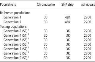
Simulated genomic data consisted of the SNP marker genotypes of individuals in the last nine generations. It included 24 300 animals genotyped with a panel of 42 000 SNP markers (42K) with an equal number (2700 genotyped animals) in each generation. To investigate the quality of genotype imputation over generations, genotyped animals were divided into a reference and testing (imputation) data sets. Three reference population structures were investigated: (1) fixed reference population that included only animals in generations 1 and 2; (2) reference population that included animals in generations 1 and 2 and was updated with an additional 1% of top animals in following generations; and (3) reference population that included animals in generations 1 and 2 and was updated with an additional 5% of top animals in following generations. Thus, the reference population included at least 5400 genotyped animals for 42K SNP marker panel. For the first scenario (fixed reference population), the testing populations were each of the remaining seven generations (generations 3 to 9). For scenarios 2 and 3 (updated reference populations), the testing population consisted only of generation 9. In the testing populations, only 3000 evenly distributed SNP markers were kept and the remaining 39 000 SNP genotypes were masked to mimic a scenario of low-density genotyping with a 3K SNP marker panel. In all cases, FImpute v2.2 was used to carry out the imputation of missing SNP genotypes. In all scenarios only population-based information was used for imputation.
Accuracy of imputation
True and imputed genotypes at a given locus were coded 0, 1 and 2 for A1A1, A1A2 and A2A2, respectively. True and imputed genotypes were deemed concordant if they matched perfectly. To access the accuracy of the imputation, the overall error rate (OER), and the average concordance rate (CR) were calculated over all imputed SNP marker genotypes. The OER consisted of calculating the percentage of the non-concordant genotypes. The CR was calculated based on the number of errors counted at an imputed genotype that was equal to 0 when true and imputed genotypes were identical, 1 if the true genotype was homozygous and the imputed genotype was heterozygous (or vice versa), and 2 if true and imputed genotypes were equal to the alternative.
 $${\rm OER} \;{\equals}\;\left( {{{{\rm Number}\,{\rm of}\,{\rm non}\,{\rm {\minus}}\,{\rm concordant}\,{\rm genotypes}} \over {{\rm Total}\,{\rm number}\,{\rm of}\,{\rm masked}\,{\rm SNPs}\,{\rm genotypes}}}} \right){\times}100$$
 $${\rm CR}\,{\equals}\,\!\left(\!\!{1{\minus}{{{\rm Number}\,{\rm of}\,{\rm errors}} \over {{\rm Total}\,{\rm number}\,{\rm of}\,{\rm masked}\,{\rm SNPs}\,{\rm genotypes}\,{\rm {\times}}\,{\rm 2}}}} \!\right)\!{\times}\!100$$
In addition, accuracy was dissected into the two types of imputation errors, which could have different implications in association and selection studies: (1) major allele homozygotes to minor allele homozygotes and vice versa (Miss 2); and (2) homozygotes to heterozygotes and vice versa (Miss 1). The former type is potentially riskier as it most likely alters the allele frequencies or even switches major with minor alleles (Huang et al., Reference Huang, Wang and Rosenberg2009). All imputation accuracy measurements were based on an average of five replicates.
Estimation of GEBVs
In order to evaluate the effect of multi-generational imputation of SNP marker genotypes on the accuracy of GS, GEBVs were estimated using true and imputed genotypes via regression-based model (BayesA) and variance component-based approach (GBLUP). For BayesA, the following model was used:
 $$y_{{ij}} \;{\equals}\;\mu {\plus}\mathop{\sum}\limits_{j\;{\equals}\;1}^p {X_{{ij}} g_{j} {\plus}e_{i} } $$
where y ij is the true BV of animal i in the reference (training) population, μ the overall mean, X ij the genotype for animal i at locus j (j=1,2, … p), where p is the number of SNPs, g j the jth SNP effect, and e i the residual term.
In matrix notation, the model in (1) can be rewritten as:
 $${\mib{y}} \;{\equals}\;\mu {\bf{1}} _{n} {\plus}{\mib{Xg}} {\plus}e$$
where y is the vector of observations, g the vector of SNP effects; X the matrix of SNP genotypes, e the vector of residual terms and n the number of animals in the training population. A hierarchical Bayesian implementation was adopted. The first stage of the hierarchy consisted of the conditional distribution of the data given the parameters of the model and it was assumed to be normal:
 $$y\!\mid\!\mu ,{\mib{X}} ,{\mib{g}} ,\sigma _{e}^{2} \,\sim\,N\left( {\mu {\bf 1}_{n} \,{\plus}\,{\mib{Xg}} ,{\mib{I}} _{n} \sigma _{e}^{2} } \right)$$
In the second stage, the following priors were assumed for the model parameters
 $$\eqalignno{ & \mu \,\sim\,{\rm constant} \cr & g_{i} \,\sim\,N(0,\sigma _{i}^{2} )\;{\rm for }\;i\;{\equals}\;(1,2,\,...\,,p) \cr & \sigma _{e}^{2} \,\sim\,\chi ^{{{\minus}2}} ({\it v} _{0} ,s_{0}^{2} ) $$
Finally, prior distributions were specified for the variance of the SNP effects. A conjugate prior was assumed. Thus,
 $$\sigma _{i}^{2} \,\sim\,\chi^{{{\rm {\minus}2}}} \left( {v_{i} ,s_{i}^{2} } \right)$$
The hyper-parameters v
0, v
i
,
 $s_{0}^{2} $
and
 $s_{i}^{2} $
were set equal to 2, 0.6, 4 and 1.41e−5, respectively. The implementation of the proposed hierarchical model is straightforward as all conditional distributions are in closed form being normal for the position parameters and scaled inverted χ
2 for the dispersion components.
When GBLUP was used, the following model was implemented to estimate GEBVs
 $${\mib{y}} \;{\mib{{\equals}}}\; \mu {\bf{1}} _{n} \,{\plus}\,{\mib{Zu}} \,{\plus}\,{\mib{e}} $$
where u is the vector of GEBVs and Z a known incidence matrix with the appropriate dimensions that relates the phenotype to the BVs. Everything else is as defined before. It is worth mentioning that the vector u includes training and validation animals. Further, it was assumed that:
 $${\mib{y}}\!\mid\!\mu ,{\mib{u}} ,\sigma _{e}^{2} \,\sim\,N(\mu {\bf 1}_{n} {\plus}{\mib{Zu}} ,{\mib{I}} _{n} \sigma _{e}^{2} ),\; {\rm and}$$
 $$\eqalignno{ & {\mib{u}} \,\sim\,N({\bf 0},{\mib{G}} \sigma _{u}^{2} ){\rm } \cr & \sigma _{e}^{2} \,\sim\,\chi ^{{{\minus}2}} ({\it v} _{0} ,s_{0}^{2} ) \cr & \sigma _{u}^{2} \,\sim\,\chi ^{{{\minus}2}} ({\it v} _{u} ,s_{u}^{2} ) $$
The hyper-parameters v
0, v
u
,
 $s_{0}^{2} $
and
 $s_{u}^{2} $
were set equal to 2, 0.6, 2 and 0.4, respectively.
G
is the matrix of genomic (realized) additive relationship between animals in the training and validation sets. It was computed based on the observed SNP genotypes (coded 0, 1 and 2) using the following formulae (VanRaden, Reference VanRaden2008).
 $${\mib{G\;{\equals}\;w}} '{\mib{w\,/\,}} \left[ {2\mathop{\sum}\limits_{i\;{\equals}\;1}^p {p_{i} \left( {1{\minus}p_{i} } \right)} } \right]$$
where W is the matrix Z of observed SNP genotypes adjusted by the minor allele frequencies (MAFs).
The implementation of the model in equation (3) is identical to the classical mixed linear model, except that the average additive relationship matrix ( A ) is replaced by G . For both models, a full Bayesian implementation was adopted. A single chain of 100 000 iterations was implemented where the first 20 000 rounds were discarded as burn-in period. Using GBLUP, the GEBVs were directly obtained after solving the system of equations. Using BayesA, the estimated GEBV for each animal was computed as the sum (over all SNPs) of the product of each SNP effect and its associated genotype.
 $$GEBV_{i} \;{\equals}\,\mathop{\sum}\limits_{k\;{\equals}\;1}^p {x_{{ik}} \hat{g}}_k$$
Accuracy was calculated based on the correlation between true BVs and GEBVs and was averaged over five replicates.
Results and discussion
Imputation accuracy
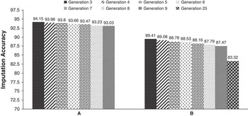
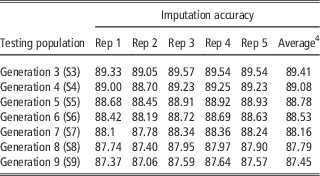
Table 2 presents a summary statistic of the imputation parameters for the different simulation scenarios with the fixed reference population. In all cases, generations 1 and 2 were part of the reference population and consisted of 5400 individuals genotyped with the high-density SNP panel (42K chip). The testing data set consisted of generations 3 to 9. Each of these testing generations included 2700 individuals. Only the low-density SNP genotypes (3K panel) were kept for these individuals. The remaining 39 000 SNP markers were masked and later used in the evaluation of the imputation process. Consequently, the missing rate was 92.86% across the genome and in each one of the 30 chromosomes. Imputation was conducted separately for each of the seven testing data sets (S3 to S9). Imputation accuracy was evaluated based on OER, CR, and Miss 1 and Miss 2, as defined earlier. Table 3 represents the imputation accuracy, using fixed reference population and the OER criteria. All results are based on the average of five replicates. As expected, imputation accuracy decreased with the increase in the generational interval between the reference and testing data sets. This is largely due to the fact that successive mating events lead to a reduction in size of the LD blocks which in turn will reduce the length of common haplotypes between progeny and ancestors. Thus, the remaining SNP markers in the low-density panel will over time lose their ability to predict the missing genotypes due to the decay in LD. The results of imputation accuracy are in line with the results reported by VanRaden et al. (Reference VanRaden, Van Tassell, Wiggans, Sonstegard, Schnabel, Taylor and Schenkel2013). In their study, only one chromosome was simulated. The reference population consisted of 1112 animals genotyped for the HD panel (777K SNPs). Imputation for lower density panels were carried out using FImpute. Imputation accuracy was 99.96%, 99.3%, 94.7% and 91.1% when HD, 50K, 6K and 3K SNP panels were used, respectively. The imputation from the 3K panel in VanRaden et al. (Reference VanRaden, Van Tassell, Wiggans, Sonstegard, Schnabel, Taylor and Schenkel2013) is similar to our first simulation scenario (S3) where generation 3 was imputed based on genotypes in generations 1 and 2. Within these parameters, our imputation accuracy (89.4%) was similar to their results (91.1%). The slight difference could be due to the size of the reference population, the level of genetic similarity between reference and validation sets, and the larger number of progeny per sire in VanRaden et al. (Reference VanRaden, Van Tassell, Wiggans, Sonstegard, Schnabel, Taylor and Schenkel2013). Based on our results and those observed in VanRaden et al. (Reference VanRaden, Van Tassell, Wiggans, Sonstegard, Schnabel, Taylor and Schenkel2013), imputation of SNP genotypes from a very low-density panel (3K) leads to acceptable results when the reference and training populations are from adjacent generations; reflective of high genetic similarity. Furthermore, imputation accuracy increases significantly with the increase of the coverage in the SNP panels (i.e. from 50K to 777K). This is expected because the higher LD in reference and target panels and the shorter the haplotypes to be imputed. However, when the generational interval between the reference and testing populations increases, the imputation accuracy decreases as indicated in Figure 2. In this study, the imputation accuracy decreased by an average of 0.5% per generation for the first seven generations following the reference population. After seven generations, the overall decrease in imputation accuracy was 2.5%. A similar trend was observed when imputation accuracy was evaluated using the CR as presented in Figure 2.
Imputation accuracy of marker genotypes across generations using (a) the concordance rate criteria and fixed reference population (generations 1 and 2), and (b) the overall rate of errors criteria and fixed reference population (generations 1 and 2).

Layout of the different simulation scenarios including the reference and testing populations

1 S3 to S9: generations 3 to 9 were used separately as testing populations.
Imputation accuracy from lowFootnote 1 to highFootnote 2 density panels based on overall concordance rate (1-OER) for each of the seven testing populations (S3 to S9)Footnote 3

OER=overall error rate; SNP=single nucleotide polymorphism.
1 3000 SNP marker panel.
2 42 000 SNP marker panel.
3 S3 to S9: generations 3 to 9 were used separately as testing populations.
4 Results are based on five replicates.
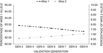
The proportion of Miss 1, as defined earlier, was always greater than Miss 2, although the latter tends to increase as the generational interval between reference and testing populations increases (Figure 3). The increase in Miss 2 is not well captured by the OER criteria and could have a substantial effect on the genome-wide association studies (GWAS) and GS. This is due to the fact that when both alleles of the SNP are incorrectly imputed, the contribution of the SNP to genetic variance and ultimately the phenotype could be reduced or even reserved. Furthermore, this type of imputation error could lead to false positive in GWAS analysis.
Percentage of one allele (Miss 1) and two alleles (Miss 2) errors across generations using fixed reference population (generations 1 and 2).

With updated reference populations, the decay in imputation accuracy was smaller as presented in Supplementary Figure S1. In fact, when the reference population consisted of generation 1 and 2 plus an additional 1% of the top animals in the following six generations (generations 3 to 8), the imputation accuracy for the testing population (generation 9) increased to 87.97%. This increase translates in a 36% reduction in the decay of imputation accuracy between generations 3 and 9 compared with the fixed reference population scenario. When the updating of the reference population consisted of an additional 5% of animals in generations 3 to 8, the imputation accuracy for the 9th generation increased to 88.74%. It is worth mentioning that across scenarios, the imputation accuracy was, as expected, higher for SNPs with low MAFs. In fact, the imputation accuracy was 0.96 for SNPs with MAF between 0.1 to 02 compared with 0.93 for SNPs with MAF ranging from 0.4 to 0.5 for generation 3 and 0.95 and 0.92 for generation 9. Therefore, the lower the MAF, the more likely it is that the most common allele will be correct (Supplementary Figure S2).
These results represent a snapshot of imputation accuracy and although they highlight a trend, the absolute numerical values depend on a multitude of factors including: (1) imputation algorithm and software package used (Browning and Browning, Reference Browning and Browning2007; Hao et al., Reference Hao, Chudin, McElwee and Schadt2009; Howie et al., Reference Howie, Donnelly and Marchini2009; Nothnagel et al., Reference Nothnagel, Ellinghaus, Schreiber, Krawczak and Franke2009; Ma et al., Reference Ma, Brøndum, Zhang, Lund and Su2013), (2) population structure and size and genetic similarity between the reference and testing populations (Druet and Georges, Reference Druet and Georges2010; Zhang and Druet, Reference Zhang and Druet2010) and (3) density and distribution of SNP markers in the low-density panel (Druet et al., Reference Druet, Schrooten and de Roos2010; Weigel et al., Reference Weigel, de los Campos, González-Recio, Naya, Wu, Long, Rosa and Gianola2010; Khatkar et al., Reference Khatkar, Moser, Hayes and Raadsma2012). Several authors (Berry and Kearney, Reference Berry and Kearney2011; Hoze et al., Reference Hoze, Fouilloux, Venot, Guillaume, Dassonneville, Fritz, Ducrocq, Phocas, Boichard and Croiseau2013; Brondum et al., Reference Brondum, Guldbrandtsen, Sahana, Lund and Su2014) have reported improved imputation accuracy with the increase of the size of the reference population. Although it is the general trend that the more animals genotyped with the high-density panel, the higher the imputation accuracy from 3K to 50K panels, it seems that the accuracy tends to reach a certain plateau after a specific proportion of population has been genotyped with the high-density panel as reported by Wang et al. (Reference Wang, Woodward, Bauck and Rekaya2012). Thus, it does not seem that the reference population used in this study will have major impact of the results. However, it is very likely that the population structure and the genetic relatedness among animals in the reference and testing populations have impacted the results.
Finally, imputation accuracy is largely data dependent. Thus, trying to compare results across studies is difficult. Nevertheless, general trends could be captured as a function of population size, missing rate of genomic data, MAF and levels of LD between markers. In addition, accuracy reported as correct percentage cannot be compared across data sets with different MAF distributions.
Estimation of GEBVs
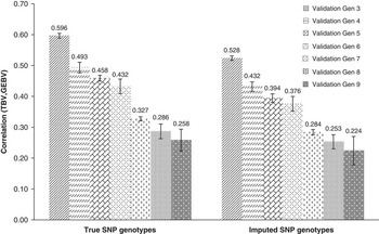
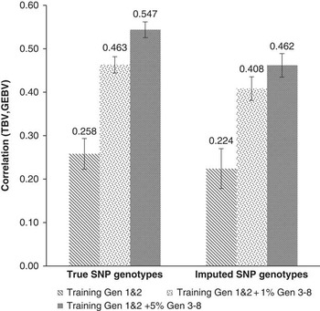
Figure 4 presents the accuracies of estimated GEBVs of the validation animals when the training population was fixed using the true and imputed SNP genotypes implemented via the BayesA method. In all cases, the accuracy was, as expected, higher using the true SNP genotypes. Such superiority ranged from 11% (generation 3) to 15% (generation 7). At least for the four generations (3 to 7) after the reference population, it could be deduced that the compounding of imputation errors has led to a 1% to 2% decrease in GEBVs accuracy per generation. However, using the true or the imputed genotypes, the accuracy decayed with the increase of the generational interval between the training and validation populations. In fact, the accuracy dropped from 0.60 to 0.26 and 0.52 to 0.22 between generations 3 and 9 using the true and imputed SNP genotypes, respectively. These results indicate that the decrease in accuracy is mainly due to the increase in genetic dissimilarity (distance) between training and validation sets, rather than the accuracy of the SNP genotypes. When the training population consisted of generations 1 and 2 and was updated with either 1% or 5% of top animals in following generations, the accuracy of estimated GEBVs in the 9th generation has improved substantially (Figure 5). With 1% updating of the training population, the accuracy increased to 0.46 and 0.41 from 0.26 and 0.22 using the true and imputed genotypes, respectively. It increased to 0.54 and 0.46 when the training population was updated with an additional 5% of top animals in generations 3 to 8. These results indicated that the decay in accuracy was only 8% and 11% between generations 3 and 9 when a 5% updating scheme was adopted using the true and imputed genotypes, respectively. The small difference (8% v. 11%) again indicates that with reasonable imputation accuracies, true and imputed genotypes perform similarly, as long as the training population is appropriately updated to reflect the genetic change in the population. When the heritability was equal to 0.1 similar trend was observed. When the training population consisted of generations 1 and 2 and was updated with 5% to top animals in following generation, the accuracy of GEBVs on generation 9 was 0.36 and 0.27 using the true and imputed SNP genotypes, respectively (Supplementary Figure S3). Although these results show the importance of the size of the training population on the accuracies of GEBV as it has been shown in several other studies (Meuwissen et al., Reference Meuwissen, Hayes and Goddard2001; Goddard, Reference Goddard2009), they highlight more importantly the effect of the genetic architecture of the trait and the LD between markers and QTLs.
Accuracy of estimated genomic breeding values (GEBV) using true and imputed single nucleotide polymorphism (SNP) genotyped based on a fixed reference population and BayesA method. Bars indicate the standard errors. TBV = true breeding vale.

Accuracy of estimated genomic breeding values (GEBV) in generation 9 using true and imputed single nucleotide polymorphism (SNP) genotypes and different training populations. Bars indicate the standard errors. TBV = true breeding vale.

When comparing both estimation methods, there is not a large difference in accuracy using BayesA or GBLUP approaches (Supplementary Figure S4). Using either the true or imputed SNP genotypes, the accuracies are basically the same between the two methods. Theoretically one could postulate the possibility of differences between the two methods in their sensitivity of errors in the imputed genotypes due to the manner in which they estimate SNP effects. However, that was not supported at least by the results of the present study.
Conclusions
GS is fast becoming a standard tool in several livestock improvement programs. Its superiority to classical BVs estimation methods is unquestionable. However, this performance is possible only when a certain set of conditions is met. One of these conditions is the availability of dense SNP marker maps. In spite of the continuous decrease in genotyping cost, it remains too expensive for large scale use in several segments of the livestock industry. To balance these two conflicting requirements, imputation of un-typed SNP genotypes in low-density and low-cost SNP panels has become an acceptable option. Genotype imputation provides an attractive and cost effective tool for large scale implementation of GWAS and GS in animal and plant applications. Even with low-density panels with a few thousand SNPs, high accuracies are possible, especially when the number of generations between reference and testing population is small. As the number of generations increases, the imputation accuracies decay, although not at an alarming rate based on the results of this study. However, under different population structures, the decay in imputation accuracy could be substantial. Furthermore, a reasonable updating of the reference population will significantly reduce, or even eliminate, the decay in imputation accuracy over generations. Although pedigree information was not used in this study, it is likely to have an impact on the imputation accuracy, especially in scenarios where LD is low.
More importantly, the use of these imputed genotypes in GS will have little to no effect on the accuracy of estimated GEBVs as long as a reasonable updating of the training population is implemented. This result holds true even after several rounds of selection. These results validate to a large extent current industry practices of GS. However, this will hold true only with a comprehensive updating of reference and training populations with new high-density genotyped animals. It could have been informative to compute the decay of LD between markers and QTLs but that was not possible due to the limitations of the software.
Supplementary material
To view supplementary material for this article, please visit http://dx.doi.org/10.1017/S1751731115002906