





I
Financial crises disrupt credit intermediation and can impose large and persistent costs on the real economy. In response, central banks frequently intervene as lenders of last resort (LLR), providing liquidity to financial institutions in order to stabilize the banking system and prevent widespread failures. While the short-run objective of these policies is well understood, namely preventing bank runs and restoring financial stability, their broader real effects remain less clear. In particular, an open question is whether lender-of-last-resort interventions merely mitigate short-term financial distress or whether they can shape the longer-run geography of economic activity and labor market outcomes.
Evaluating the real effects of LLR policies is difficult in modern settings because policy responses typically occur at the national level and are endogenous to evolving economic conditions. Changes in monetary policy often coincide with fiscal responses, regulatory reforms and macroeconomic shocks, making it difficult to isolate the causal effect of financial stabilization. Historical episodes in which policy responses differed across otherwise similar regions therefore provide particularly valuable opportunities to study the economic consequences of central bank intervention. This article shows that lender-of-last-resort intervention during the Great Depression not only stabilized banks and local manufacturing activity but also had persistent effects on individual labor market trajectories and geographic mobility.
This article studies the real effects of lender-of-last-resort policy using a well-known natural experiment from the early years of the Great Depression. During the banking panic of 1930, the Federal Reserve Bank of Atlanta aggressively extended liquidity to member banks, adhering to Bagehot’s principle of lending freely to solvent but illiquid institutions. In contrast, the Federal Reserve Bank of St. Louis adopted a far more restrictive approach, providing little emergency liquidity during the crisis. Because the Federal Reserve district border divided otherwise similar counties within states such as Mississippi and Tennessee, this divergence generated quasi-experimental variation in access to liquidity support.
A substantial literature has exploited this policy divergence, and it has examined a wider set of outcomes than banking alone. Richardson and Troost (Reference Richardson and Troost2009) document that banks in the Atlanta district of Mississippi experienced significantly lower failure rates during the panic of 1930, and, tracing the real consequences of the panic, show that credit availability and the county-level volume of wholesale trade contracted less on the Atlanta side of the border. Jalil (Reference Jalil2014) extends the analysis beyond Mississippi to all counties within 50 miles of the Atlanta district border and confirms that bank suspension rates were consistently lower inside the district in 1929 and 1930. Ziebarth (Reference Ziebarth2013) uses plant-level data from the Census of Manufactures to show that the resulting variation in bank failures reduced physical output in Mississippi manufacturing and discusses the associated county-level labor market effects, while Hansen and Ziebarth (Reference Hansen and Ziebarth2017) draw on Moody’s data covering manufacturing as well as other industries to document how banking distress increased business exit and disrupted credit relationships. Freedman (Reference Freedman2017) studies Depression-era Mississippi and shows that local economic interventions in this period had effects on a range of labor market outcomes that persisted for decades. Most recently, Choi and Huang (Reference Choi and Huang2025) revisit the Atlanta–St. Louis experiment using newly digitized bank-level balance sheet data from the Rand McNally Bankers Directory matched to census microdata, and show that the effects of the Atlanta Fed’s liquidity support on bank exits, credit provision and post-crisis household outcomes were concentrated in less competitive, rural banking markets.
Relative to this body of work, the contribution of this article is to trace the consequences of lender-of-last-resort policy through to individual workers over the following decade. Existing studies measure outcomes for banks, plants, firms and county aggregates, largely within the crisis years themselves; what has remained unexplored is whether workers exposed to financial stabilization followed persistently different careers: whether they remained in manufacturing, how their earnings capacity evolved and whether they stayed in or left the affected regions. Yet financial crises ultimately affect households through labor markets: if stabilizing banks preserved local employment opportunities, LLR policies may have had lasting effects on individuals’ sectoral attachment and geographic mobility long after the panic subsided.
This article studies these longer-run labor market consequences of financial stabilization. I combine newly digitized county-level manufacturing data with linked individual-level census records from 1930 and 1940 to examine how exposure to lender-of-last-resort intervention affected both local economic activity and individual labor market trajectories. Leveraging the quasi-experimental variation created by the Atlanta Federal Reserve district border, I compare counties just inside the Atlanta district with neighboring counties under the jurisdiction of the St. Louis Fed.
The analysis proceeds in three steps. First, I document that access to lender-of-last-resort intervention significantly reduced bank failures during the early years of the Depression. Counties located within the Atlanta district experienced bank failure rates between 8 and 13 percent lower than adjacent counties outside the district. These results are consistent with the historical evidence that the Atlanta Fed actively supplied liquidity to distressed banks during the crisis.
Second, I examine the effects of these banking differences on local economic activity. Using newly digitized county-level data from the Census of Manufactures, I show that counties exposed to Atlanta’s liquidity support experienced substantially stronger manufacturing performance in the early 1930s. Between 1929 and 1931, treated counties exhibited significantly higher manufacturing output, employment and establishment counts relative to neighboring counties outside the Atlanta district. These results suggest that stabilizing the banking sector mitigated the contraction in local manufacturing activity during the Depression.
Third, I examine the long-run labor market consequences of these policies using linked individual-level census records. I find that residents of counties exposed to Atlanta’s lender-of-last-resort policy were significantly more likely to remain employed in manufacturing by 1940 and less likely to migrate across state lines. These effects are concentrated among younger and less-educated workers, suggesting that access to financial stabilization influenced the long-run allocation of labor across sectors and locations. Taken together, the results indicate that early intervention in financial markets can shape the spatial distribution and composition of employment long after the initial crisis has passed.
This article advances the literature on the Atlanta Federal Reserve experiment in three ways. First, it provides the first evidence on the decade-long, individual-level labor market consequences of Depression-era financial stabilization. Prior work has established effects on bank survival and credit (Richardson and Troost Reference Richardson and Troost2009; Jalil Reference Jalil2014), on plant-level manufacturing output and contemporaneous county labor markets (Ziebarth Reference Ziebarth2013), on business exit across manufacturing and other industries (Hansen and Ziebarth Reference Hansen and Ziebarth2017), and on county-level trade and commerce (Richardson and Troost Reference Richardson and Troost2009). By following 1.88 million individuals from 1930 to 1940 with linked full-count census records, I show that lender-of-last-resort intervention also shaped workers’ sectoral attachment, occupational income and migration decisions.Footnote 1
Second, the article broadens the geographic scope of the downstream, real-outcome evidence. Whereas the manufacturing and firm-level analyses in Richardson and Troost (Reference Richardson and Troost2009) and Ziebarth (Reference Ziebarth2013) focus on Mississippi, I follow Jalil (Reference Jalil2014) in using all counties within 50 miles of the Atlanta district border, spanning multiple state borders and neighboring Federal Reserve districts. This design assesses the generalizability of the Mississippi findings and permits within-state comparisons in Mississippi, Tennessee and Louisiana; I also report Mississippi-only estimates throughout as robustness checks, consistent with the original design of Richardson and Troost (Reference Richardson and Troost2009).
Third, the article speaks directly to the mechanism by integrating measures of financial dependence into the spatial identification strategy. I merge county-level industry composition with two measures of external finance dependence (a contemporaneous Commerce Department credit survey of small and medium manufacturers and the structural proxies of Rajan and Zingales (Reference Rajan and Zingales1998)) and show that manufacturing declines were concentrated where firms depended on bank credit. This provides direct evidence that the lender-of-last-resort effects documented here and in prior work operated through the credit channel, advancing beyond earlier studies that lacked measures of financing constraints at the local level.
The remainder of the article proceeds as follows. Section II provides historical background on the Federal Reserve’s response to the banking panic of 1930 and describes the institutional differences between the Atlanta and St. Louis districts. Section III introduces the data sources used in the analysis. Section IV documents the relationship between external finance dependence and manufacturing decline during the Depression. Section V presents the border design and examines the effects of lender-of-last-resort intervention on bank failures. Section VI analyzes the downstream effects on manufacturing and the long-run labor market and migration outcomes using linked census data. Section VII concludes.
II
Banking crises
The events of the Great Recession (2007–9), a financial crisis followed by a deep economic recession and a slow recovery, renewed interest in the study of how financial market distress affects households and firms. The Great Depression (1929–37) serves as the most pertinent historical comparison to the economic challenges faced in the late 2000s. Initiated by a stock market crash in 1929 and exacerbated by subsequent banking failures, the Depression remains a focal point in US economic history and macroeconomic policy. Notably, Friedman and Schwartz (Reference Friedman and Schwartz1963) and Bernanke (Reference Bernanke1983) identify bank panics as pivotal in shaping the economic downturn and determining the Depression’s duration and severity. From a policy standpoint, discerning the causes of financial institution failures and the efficacy of preventive measures is crucial for financial market regulators and central banks.
Two main hypotheses underpin the causes of bank failures during the Depression in the United States. The first hypothesis posits that banks faced insolvency as the assets they held (primarily mortgages, business loans and bonds) diminished in value (Temin Reference Temin1976; White Reference White1984; Calomiris and Mason Reference Calomiris and Mason2003). In essence, banks had made risky investments before 1929: excessive loans to businesses that would later collapse, to stock speculators who suffered significant losses in the 1929 crash, and mortgages during the post-World War I construction boom. Empirical support for this solvency hypothesis manifests in various ways, such as state-level bank failures correlated with economic and loan characteristics, bank-level data on loan quality, and trends in bond yields. Typically, these studies consider the probability or severity of bank suspensions, concluding that underlying economic shocks are potent predictors of bank failure. They suggest that liquidity-assistance policy interventions would likely have had limited impact during the Depression.
The second hypothesis, the illiquidity hypothesis, contends that a surge in withdrawals by panic-stricken depositors crippled the banking sector. The stock market crash sowed doubts about future economic prospects (Romer Reference Romer1990). Additionally, news about the failures of major, interconnected institutions stirred concerns about the banking sector’s stability. Consequently, public trust eroded, leading to a rush on banks, which, unable to liquidate assets swiftly, had no choice but to halt operations (Friedman and Schwartz Reference Friedman and Schwartz1963; Wicker Reference Wicker2000). Under this theory, the crisis might have been mitigated had the Federal Reserve acted as a lender of last resort, offering cash to banks in exchange for illiquid assets at non-fire sale prices. Some critiques center on the Federal Reserve’s perceived inaction during the Depression based on this perspective.
Both hypotheses hold conceptual and empirical merit, contingent on the specific timeframe, geographical context and granularity of the data. No singular cause can encapsulate the magnitude of banking panics during the Great Depression. The most insightful evidence on the solvency and liquidity channels’ relative importance comes from Richardson (Reference Richardson2007). Utilizing quarterly bank-level data from 1929 to 1933, he observes a temporal evolution in bank failures: initially, small rural banks faced increasing failure rates. The collapse of Caldwell and Company and the Bank of the United States in 1930 triggered bank runs. By 1931, following Britain’s exit from the gold standard and declining asset values, the majority of failing banks were indeed insolvent. Nearly three-fourths of these institutions were deemed insolvent, with one-fourth solvent and either resuming business or merging. Among those that suspended operations, half did so due to depositor withdrawals.
What was the scope of Federal Reserve intervention?
The initial response of the Federal Reserve to the Depression has been a subject of criticism, especially its support (or lack thereof) for the money supply and banking institutions. However, pinpointing its direct impact is intricate due to potential responses from households and local bodies. The ideal approach would involve comparing regions with analogous economic trajectories but divergent policy responses during the Depression. Mississippi serves as a pertinent case study in this regard, with its northern and southern counties subjected to distinct policy regimes up until 1931 (Richardson and Troost Reference Richardson and Troost2009; Ziebarth Reference Ziebarth2013; Jalil Reference Jalil2014).
The southern counties of Mississippi fell under the purview of the Atlanta Federal Reserve Bank (6th District). Atlanta leaders adhered to Bagehot’s rule, a doctrine advocating that central bankers should provide credit to illiquid but solvent institutions during financial upheavals, thereby preventing losses from runs on otherwise healthy banks. Gamble (Reference Gamble1989), in his historical overview of the Atlanta Federal Reserve Bank, recounts instances where bank officials physically transported currency into banks to reassure apprehensive depositors of the bank’s solvency. Conversely, in the north, the St. Louis Federal Reserve Bank (8th District) championed the ‘Real Bills’ perspective, asserting that credit supply should diminish during downturns, as reduced economic activity necessitated less credit. This stance persisted until the summer of 1931.Footnote 2 Therefore, during the Depression’s initial two years, banks in Mississippi experienced two contrasting policy approaches. What were the implications?
Drawing from bank-level and county-level data, Richardson and Troost (Reference Richardson and Troost2009) unveil compelling findings. Banks in the 6th District counties of Mississippi consistently outperformed their counterparts in the 8th District in terms of survival rates, credit availability and commercial activity, particularly during the panics of 1930-1. Their research suggests that broad application of LLR policies might have mitigated the onset of banking panics. Broadening the analysis to encompass the entire border of the 6th District, Jalil (Reference Jalil2014) investigates whether bank performance in counties within 50 miles of this boundary depended on the specific Federal Reserve policy regime. Utilizing county-level banking data, he discerns that bank suspension rates in 1929 and 1930 were consistently lower inside the 6th District compared to adjacent counties just beyond the border.Footnote 3
Banking panics and local economic outcomes
Bank closures carry direct costs, such as the wealth loss for depositors who only recover a portion of their claims after a bank’s liquidation. However, this is merely one avenue through which bank failures can adversely affect local economies. An alternative channel is the escalation of financial intermediation costs (Bernanke Reference Bernanke1983). In an atmosphere riddled with uncertainty, banks lean towards risk aversion, investing predominantly in secure assets and showing hesitancy in extending credit, even to creditworthy businesses (Cornett et al. Reference Cornett, McNutt, Strahan and Tehranian2011). Consequently, these businesses curtail hiring and production. When these firms seek funds for investment or debt refinancing, the absence of willing lenders leads to a decline in their output.
The experimental scenario in Mississippi, combined with the Atlanta Federal Reserve border, offers a framework to investigate the influence of bank failures on local economic conditions. Ziebarth (Reference Ziebarth2013) assembles plant-level data from the Census of Manufactures during the Depression and employs a difference-in-differences approach to juxtapose plants in northern and southern Mississippi. His findings reveal a 37 percent reduction in physical output in the north with no discernible impact on total workforce numbers. This effect predominantly arises from the intensive margin. When viewed at the county level, he finds a pronounced negative impact on the number of workers. Related work by Hansen and Ziebarth (Reference Hansen and Ziebarth2017) examines how banking distress altered firms’ credit relationships and business dynamics during the Depression. Using detailed firm-level data, they show that bank failures disrupted existing lending relationships and increased business exit among financially dependent firms, highlighting an additional channel through which local banking crises propagated to real economic activity.
Recent work also provides complementary evidence on the microeconomic transmission of banking distress to real activity in earlier periods. Using newly assembled national data from the Progressive Era (1900–29), del Angel et al. (Reference del Angel, Richardson and Gou2024) show that bank failures causally increased bankruptcies among firms that depended on commercial banks for short-term credit, while firms that were largely bank-independent (primarily large manufacturers with access to retained earnings and capital markets) were largely insulated. They demonstrate that credit supply disruptions operated through clearly identifiable bank-firm linkages, rather than through broad aggregate demand channels. Their findings underscore that bank failures mattered precisely because of firms’ reliance on relationship banking for working capital, reinforcing the importance of financial intermediation in shaping real outcomes even before the Great Depression.
III
I briefly describe the main sources of county, firm and individual-level data in this section. For a detailed review of the sources, please see Online Appendix A.
Banking and finance
To assess local credit conditions during the Depression, I draw on a 1934 US Commerce Department survey of over 6,000 small and medium-sized manufacturers, which found widespread credit use and credit difficulties: over 80 percent reported that commercial banks provided the main source of external funding, and 45 percent of borrowing firms reported trouble accessing loans (US Census Bureau 1935). I construct an industry-level measure of credit constraint (the proportion of all firms that reported credit difficulty) from this survey and aggregate it to the county level using output-weighted averages.Footnote 4 While informative, the survey reflects conditions several years into the Depression and may understate constraints in industries where many firms had already failed. To address this limitation, I complement it with the measure of industry-level external financial dependence from Rajan and Zingales (Reference Rajan and Zingales1998), which captures structural financing needs computed using accounting data from publicly traded firms in the 1980s. I further incorporate county-level data on banking disruptions using bank suspension data from the Federal Deposit Insurance Corporation and newly digitized balance sheet data from the Office of the Comptroller of the Currency (Federal Deposit Insurance Corporation 1992; United States Office of the Comptroller of the Currency 1920–32).
Manufacturing and industry composition
To construct measures of local industrial activity and composition, I digitize county-level output, employment and establishment count data from the Census of Manufactures for 1927–35, including a 1927 special tabulation of plant counts by industry and county published in the Market Data Handbook (US Census Bureau 1937; Stewart Reference Stewart1929). I transform the establishment counts by industry to the 15-sector classification used in the 1935 Credit Survey and convert these counts into economic shares using state-industry averages of output, employment and wages, thereby accounting for variation in establishment size across sectors. Due to census confidentiality thresholds, coverage is incomplete in low-manufacturing counties; I address this by restricting to a balanced panel across census years. I construct outcomes including log output, log employment and log wages. Baseline county characteristics are well balanced across the border, though manufacturers just outside the boundary were marginally larger on average.
Linked decennial censuses, 1930–40
Data regarding manufacturing workers comes from the 100 percent count US census records. This article focuses on working-age adults (ages 18–55) in Mississippi, Tennessee and Louisiana – the three states bisected by the Atlanta Federal Reserve border. I used the crosswalks provided by the Census Tree Project (Price et al. Reference Price, Buckles, Haws and Wilbert2023) and IPUMS publicly available census data (Ruggles et al. Reference Ruggles, Nelson and Sobek2024) to link records over time.Footnote 5 In total, the 1930–40 sample includes over 1.88 million individuals, with 65 percent living in counties within the Atlanta district. This linked sample covers roughly 51 percent of the manufacturing workforce in 1930 in those states but is not perfectly representative. To address this issue, I use inverse probability weighting in my empirical analysis, creating weights after predicting the characteristics associated with a successful link. I construct four primary outcome variables: a binary variable taking the value of 1 if the individual reported working in the manufacturing sector in 1940, the logarithm of the change in the individual’s occupational income score, and two binary variables indicating inter-county and inter-state migration.
Other data
Using the Geographic Information Systems (GIS) software, I identify counties within a 50-mile radius of all Federal Reserve districts. These bordering counties were further segmented based on their proximity to specific Federal Reserve districts (e.g. Atlanta – St. Louis segment) as shown in Figure 1. My approach closely mirrors the method employed by Jalil (Reference Jalil2014). For robustness checks, I transcribed the 1927 consumer markets map from the US Department of Commerce Market Data Handbook. This map categorizes counties into 632 distinct consumer markets, which were crafted from a consumer-centric viewpoint based on an initiative by the International Magazine Company to optimize sales efficiency. The selection of trading centers was based on parameters like population, geography, economic sources, transportation and trade channels. Lastly, I use New Deal county-level Reconstruction Finance Corporation (RFC) and Agricultural Adjustment Administration (AAA) expenditure data collected by Fishback et al. (Reference Fishback, Kantor and Wallis2003) in various robustness exercises.
Counties around the Atlanta Federal Reserve district border

Figure 1 Long description
The map shows the southeastern United States with state outlines. North is at the top. Counties within 50 miles of the Atlanta (6th) district border are shaded by border segment and by side of the border: Atlanta–St. Louis segment. This is the longest segment. It runs west across Tennessee, then south through Mississippi, then west across southern Mississippi. Atlanta-side counties lie to the east and south of the line. St. Louis-side counties lie to the north and west.Atlanta–Cleveland segment. This is a short segment in eastern Tennessee and southeastern Kentucky.Atlanta–Richmond segment. This segment runs southeast from the Tennessee–North Carolina area along the Georgia–South Carolina border to the Atlantic coast.Atlanta–Dallas segment. This segment is in Louisiana. Atlanta-side counties lie to the east and Dallas-side counties to the west. Uncoloured areas lie more than 50 miles from the district border.
Summary statistics
Table 1 presents the summary statistics. Overall, county-level banking variables are available for 365 border counties across nine years and for 364 counties for a single year (1934, due to missing bank data for one county). The roughly 1,000 observations for manufacturing span between 190 and 210 border counties reporting manufacturing activities biennially from 1927 to 1935.
Summary statistics

Table 1 Long description
Two panels report summary statistics using columns for count, mean, sd, p5, p25, p50, p75, and p95. Panel A covers county level banking, manufacturing, and related measures, with most banking rows having count 3,650. Active banks have mean 3.51, sd 2.57, p5 1.00, p25 2.00, p50 3.00, p75 5.00, and p95 9.00. Suspended banks are mostly zero at the median, with means of 0.18 for all, 0.03 for national, and 0.14 for state; p95 is 1.00 for all and state and 0.00 for national. Active deposits in millions have mean 2.60 and p50 0.91, while suspended deposits in millions have p50 0.00 across all, national, and state; p95 is 0.36 for all, 0.00 for national, and 0.22 for state. Capitalization ratio has count 1,840 with mean 0.15 and p50 0.13; loan growth for 1924 to 1929 has count 168 with mean 0.11 and p50 0.10. Manufacturing measures include output in millions with count 1,013 and p50 1.33, wages in millions with count 1,013 and p50 0.28, establishments with count 1,023 and p50 16.00, and wage earners in thousands with count 1,021 and p50 0.50; borrower difficulty and RZ difficulty each have count 356 with p50 values 0.48 and 0.21. Panel B summarizes linked census variables with observations 1,883,289, including indicator rows with p50 values of 0.00 for manufacturing in 1930 and 1940, 1.00 for Atlanta, native, male, and white, and 0.00 for urban, moved counties 1930 to 1940, and moved states 1930 to 1940; years of schooling has count 1,856,465 with mean 7.59 and p50 8.00, and age in 1930 has mean 32.86 and p50 32.00.
Notes: Panel A presents the summary statistics for all counties within 50 miles of the Atlanta Federal Reserve district border (see Figure 1). Banks (count) and Deposits (millions of nominal dollars) are reported annually between 1926 and 1936. Capitalization ratio is defined as the total surplus and profits divided by assets for nationally chartered banks in 1928. Loan growth is change between the log of all loans between 1924 and 1929 for nationally chartered banks. Loans, surplus and total assets come from the Office of the Controller of Currency. Output (millions of nominal dollars), Wages (millions of nominal dollars), Establishments (count) and Workers (thousands) come from the Census of Manufacturing, reported biennially between 1927 and 1937. Borrower-Difficulty is an industry-weighted share of small and medium manufacturers facing credit difficulties. RZ-Difficulty is an industry-weighted external capital dependency measure from Rajan and Zingales (Reference Rajan and Zingales1998). Panel B presents the summary statistics of linked census data in Mississippi, Tennessee and Louisiana between 1930 and 1940. See text for details.
Across counties, there is a pronounced negative correlation between manufacturing activity and bank failures. Figure 2 illustrates a binned scatter plot of county-level changes in the logarithm of nominal per-capita manufacturing output between 1933 and 1929 (y-axis) against the cumulative number of bank suspensions as a proportion of all 1927 banks (x-axis) in all counties with at least one suspended bank and manufacturing activity in both 1933 and 1929 (totaling 1,623 counties). On average, a 10 percentage point increase in bank failure is associated with 2 log point decrease in manufacturing output across counties.
Manufacturing decline during the Great Depression and banking failures

IV
The empirical analysis proceeds in three steps. First, I establish that external finance dependence is a key predictor of manufacturing decline during the early Depression, using industry-level credit survey data and pre-Depression manufacturing composition to construct county-level proxies for financial constraints. Second, I exploit the Atlanta Federal Reserve’s border discontinuity to show that counties within its jurisdiction experienced significantly fewer bank failures during 1929–30, consistent with more aggressive LLR intervention. Third, I examine downstream effects on firms and workers, finding that treated counties saw greater manufacturing survival, employment retention and persistent changes in individual labor market trajectories. Together, these steps provide a unified framework linking financial frictions, central bank policy and long-run local economic outcomes.
The central hypothesis is that lender-of-last-resort policy affected the real economy through a credit channel: by keeping banks open, the Atlanta Fed preserved the supply of credit to local firms, and firms that depended on bank financing were therefore shielded from the contraction. For this mechanism to be plausible, it must first be the case that manufacturing activity during the Depression was in fact sensitive to the availability of external finance. This section tests that premise directly by asking whether counties whose manufacturing base was concentrated in credit-dependent industries experienced systematically larger declines after 1929. If credit dependence did not predict manufacturing decline, there would be little reason to expect the Atlanta Fed’s banking intervention to have had downstream real effects; if it did, then the border analysis in Sections V and VI can be interpreted through the lens of financial frictions.
Measuring a county’s exposure to financial constraints requires a measure of how much its industries rely on external funds. I use two complementary industry-level measures, described in detail in the Online Data Appendix (Section A.1). The first, Borrower-Difficulty, is drawn from the 1935 US Commerce Department survey of small and medium manufacturers and equals the share of firms in an industry that reported difficulty obtaining bank credit. Because the survey was fielded during the Depression, it captures actual credit rationing but may be affected by the crisis itself. The second measure addresses this concern using the framework of Rajan and Zingales (Reference Rajan and Zingales1998). Rajan and Zingales measure an industry’s external finance dependence as the fraction of capital expenditures that firms cannot fund out of internal cash flow, computed from Compustat data on publicly traded US firms and summarized by industry medians. The key insight is that this dependence is a technological characteristic of an industry rather than a feature of any particular time or place. An industry like machinery, which requires large upfront investments relative to its operating cash flow, ranks as highly dependent on external finance; an industry like tobacco, with steady cash flows and modest investment needs, ranks low. Because the measure (RZ-Difficulty) reflects structural financing needs rather than Depression-era conditions, it is immune to the survivorship and timing concerns that attach to the survey measure. I aggregate both measures to the county level using the 1927 industry composition of manufacturing establishments (fixed before the Depression) so that a county’s ‘constraint’ reflects its pre-crisis industrial structure rather than any endogenous response to the downturn.
With these county-level exposure measures in hand, the natural test is an event-study design that compares outcomes in more- and less-exposed counties, year by year, relative to the eve of the Depression. This design has two attractive features. First, because exposure is fixed at its 1927 value, the interactions of exposure with year dummies trace out how the same cross-section of counties diverged as aggregate credit conditions collapsed after 1929, precisely the pattern the credit channel predicts. Second, the pre-1929 interaction provides a falsification test: if credit-dependent counties were already on differential trends before the Depression, the design would be less credible. I estimate the model on a balanced national panel of manufacturing counties using biennial data from 1927 to 1935:
 \begin{equation}S_{jk}=\alpha_j+\beta_{s(j)k}+\sum_{i=1927}^{1935}\left(\operatorname{constraint}_jT_i\right)\cdot\omega_i+X_{jk}+\epsilon_{jk}\end{equation}
where  ${T_i}$ is a year dummy taking the value of 1 if
 $i = k$ and 0 otherwise and
 $constrain{t_j}$ is a standardized (mean zero, standard deviation one) measure of credit difficulty (Borrower-Difficulty) based on the 1935 credit survey or external dependence (RZ-Difficulty) as in Rajan and Zingales (Reference Rajan and Zingales1998). I use county (
 ${\alpha _j}$) and state by year (
 $\beta_{s(j)k}$) fixed effects to account for all unobserved but static county variables and state-level trends in manufacturing. To account for differences in business failure rates based on firm size, I include terciles of average manufacturing plant size based on the number of wage earners in 1929 by year fixed effects (
 ${X_{jk}}$). The coefficients of interest are
 ${\omega _i}$, which capture the time-varying difference in outcome
 $S$ in counties based on industry-weighted credit difficulty. The omitted reference year is 1929, and I cluster the standard errors at the county level.
Table 2 displays the results when Borrower-Difficulty is used as the  $constrain{t_j}$ measure. Columns 1–4 use log output (revenue), log county manufacturing wage-earner wages, log number of establishments and the log number of wage-earners as the outcome variables, respectively. Two features of the estimates stand out. First, the 1927 interactions are small and, outside of a modest negative coefficient for the number of establishments, statistically insignificant: counties with credit-dependent industries were not on differential trends before the crash. Second, a clear divergence opens up precisely when the banking crisis takes hold. By 1931, counties with more borrowers facing credit challenges exhibited significantly worse outcomes across every margin: a one standard deviation (5.6 percentage point) increase in the share of firms reporting borrowing difficulty is associated with an 8 log point decline in total output and a 9 log point decline in the number of wage-earners employed, relative to 1929. The estimated gaps are largest in 1933, at the trough of the Depression and the peak of the banking crisis, and remain economically meaningful through 1935, indicating that exposed counties did not simply recover once the panic passed. The timing is important: the effects emerge with the banking crisis, deepen as it intensifies and persist after it, which is the pattern one would expect if the collapse of bank credit, rather than a pre-existing structural decline, drove the divergence. The results are quantitatively similar when RZ-Difficulty is used as the exposure measure (Online Appendix Table A3), which is reassuring given that the two measures come from entirely different sources and time periods and are subject to different biases.
Credit difficulty and manufacturing outcomes across US counties, 1927–35

Table 2 Long description
R
Standard errors in parentheses. * p < 0.10, ** p < 0.05, *** p < 0.01
Notes: This table reports the estimated coefficients of Equation (1) across all US counties where constraint (‘Borrower-Difficulty’) is an industry-weighted measure of credit access difficulty that uses the 1927 manufacturing industry by county establishment data and the 1935 credit survey of manufacturing industries. Controls include state by year fixed effects and average manufacturing plant size tercile by year fixed effects. Size is measured by number of wage earners in 1929. The omitted baseline interaction is 1929 across all specifications. The outcome variables come from Census of Manufactures. Samples are balanced. The time period is 1927–35 (biennially) for all specifications and the standard errors are clustered at the county level.
A remaining concern is that Borrower-Difficulty may conflate credit supply with credit demand: industries whose firms borrow heavily may simply be more cyclical, and their decline may reflect exposure to the downturn rather than rationing by banks. To separate the two, I decompose the survey measure and re-estimate Equation (1) using three alternative definitions of  $constrain{t_j}$: the share of firms that reported any borrowing (a measure of credit demand), the share of firms reporting credit difficulty and the share of borrowers reporting difficulty (measures of constrained credit supply). Figure 3 plots the estimated
 ${\omega _i}$ coefficients from the three regressions. The distinction matters. A county’s industry-weighted borrowing propensity (green line) predicts slightly better, not worse, outcomes after 1929: high-borrowing industries were not simply high-cyclicality industries. By contrast, the unwillingness of banks to extend credit (red and blue lines) predicts significantly worse outcomes after, but not before, 1929. In other words, it was not reliance on credit per se, but the inability to obtain it, that predicted manufacturing decline.
Manufacturing and industry-weighted credit difficulty measures at the county level

Figure 3 Long description
Panels and axes. The four panels plot estimated coefficients relative to 1929 for log output (a), log wages (b), log establishments (c) and log workers (d). The horizontal axis shows the census years 1927, 1929, 1931, 1933 and 1935. A dashed vertical line marks the omitted year, 1929, and a dashed horizontal line marks zero. Vertical bars show 90 percent confidence intervals.Series. Each panel has three series, one for each standardised constraint measure: difficult firms as a share of borrowers, difficult firms as a share of all firms, and borrowers as a share of all firms.1927. All three series are close to zero in every panel.Difficulty measures after 1929. The two difficulty measures fall sharply by 1931 and stay negative through 1935, recovering partly in 1935. Their troughs are about −0.09 for output, −0.14 for wages, −0.08 for establishments and −0.11 for workers.Borrowing-share measure after 1929. This measure stays at or above zero. It rises to about +0.06 for output, +0.10 for wages and +0.06 for workers by 1933–35, and stays near +0.02 for establishments.
Taken together, the results in this section establish the premise on which the rest of the article builds: manufacturing activity during the early Depression was highly sensitive to the availability of bank credit, the sensitivity emerged exactly when the banking system came under stress, and it reflects constrained credit supply rather than differential credit demand. These findings imply that policies that preserved local banking capacity had the potential to generate meaningful real effects.
V
Having established that counties with higher exposure to credit constraints experienced sharper manufacturing declines during the early Depression, I now turn to the identification of a plausibly exogenous policy intervention that alleviated those constraints. Specifically, I exploit the discontinuity at the border of the Atlanta Federal Reserve district to test whether liquidity provision stabilized the banking sector in treated counties.
Empirical design
The primary outcome of interest is the rate of bank failure. At the county level, I gauge this using two metrics: suspensions and the proportion of deposits retained by active banks at year-end, with the latter assessed against pre-Depression (1927) data on banks and total deposits. Both of these metrics are key, as banks might recommence operations after a brief suspension. However, the suspensions dataset does not differentiate between permanent liquidations and temporary suspensions. Hence, the end-of-year deposit values, reflecting more enduring banking sector shocks, act as a supplementary measure. Additionally, I create a binary variable, which is set to 1 if any bank within the county was suspended within the year and 0 otherwise, as a mechanism to mitigate the influence of outliers using the continuous variables.
I introduce various control variables in my analysis. I compute two measures to account for unobserved time-varying confounders due to fundamental banking differences between counties. First, I define the pre-Depression (1927) ‘capitalization ratio’ as the total surplus and capital divided by total assets. Higher capitalization ratios reflect lower leverage of the banking sector and a higher probability of withstanding depositor withdrawals. Second, I compute the logarithm of loan growth between 1924 and 1929. Higher loan growth could potentially correlate with decreased loan quality and a higher default rate in the 1930s. Finally, to control for non-financing industry-level time-varying confounders, I use the 1927 manufacturing revenue by industry shares in order to identify the dominant industry in each county. I interact the dominant industry dummy variable with time dummies to account for national industry trends.
I do not find strong underlying ex ante differences between counties across the border. Table 3 shows that counties on the border of the Atlanta district were similar.Footnote 6 Notably, the counties did not differ in their suspension rates as of 1927, had the same (estimated) proportion of manufacturing firms facing financial constraints, and their industrial structure was similar. There are some differences, but they are small. For example, although fewer banks were in the average county inside Atlanta, the total amount of deposits in 1928 was the same.
Covariate balance in 1927

Table 3 Long description
County averages are reported for counties within 50 miles of the Atlanta Federal Reserve district border, with columns for, All, In, Out, and, Difference. For, Deposits active minus all, the averages are 3546.18 in and 2876.15 out, with a difference of minus 670.02. For, Log pop, the averages are 9.78 in and 9.94 out, with a difference of 0.17 marked with one asterisk. For, Log Output, Log Wages, Log Wage Earners, and, Log number of Establishments, the differences are minus 0.12, minus 0.17, minus 0.30, and minus 0.17, respectively. For, Bank Suspension Rate all, Borrower Difficulty, and, RZ Difficulty, the in and out averages are 0.01 and 0.01, 0.48 and 0.48, and 0.21 and 0.20, with differences of 0.00, 0.00, and minus 0.00. Observations are 365 for All, 170 for In, 195 for Out, and 365 for Difference. Industry shares are also listed with the same columns and include, Paper and allied, Food and kindred products, Textiles, Rubber, Petroleum and coal, Forest products, Printing and publishing, Leather, Stone clay glass, Nonferrous metals, Transportation equipment, and, Miscellaneous. In the industry section, the difference is marked with two asterisks for, Forest products, at minus 0.014, and with one asterisk for, Printing and publishing, at 0.012; other listed industry differences range from minus 0.013 for, Textiles, to 0.023 for, Food and kindred products. Industry observations are 356 for All, 164 for In, 192 for Out, and 356 for Difference.
Standard errors in parentheses. * p < 0.10, ** p < 0.05, *** p < 0.01
Notes: This table reports variable averages among counties within 50 miles of the Atlanta Federal Reserve district border. Column ‘All’ reports the averages for all counties along the border and columns ‘In’ and ‘Out’ report them only for those in the district and for those outside the district, respectively. Column ‘Difference’ computes the difference and reports the T-test on the equality of means. The variables ‘Banks (active - all)’, ‘Deposits (active - all)’ and ‘Bank Suspension Rate (All)’ reported here are as of 1927 and come from the FDIC. ‘Borrower-Difficulty’ is an industry-weighted measure of credit access difficulty that uses the 1927 manufacturing industry by county establishment data and the 1935 credit survey of manufacturing industries. ‘RZ-Difficulty’ is an industry-weighted measure of external finance dependence that uses the 1927 manufacturing industry by county establishment data and industry measures derived in Rajan and Zingales (Reference Rajan and Zingales1998). Chemicals industry – zero establishments – is omitted.
I compare county-level outcome variables before and after the onset of the Great Depression across the Atlanta boundary using the following specification:
 \begin{equation}S_{jk}=\alpha_j+\beta_{s(j)k}+\sum_{i=1926}^{1933}\left(Atl_jT_i\right)\cdot\gamma_i+X_{jk}+\epsilon_{jk}\end{equation}
where  ${T_i}$ is a year dummy taking the value of 1 if
 $i = k$ and 0 otherwise and
 $At{l_j}$ takes the value of 1 if the county belongs to the Atlanta district and 0 otherwise. Like in the previous section, I use county (
 ${\alpha _j}$) and border region by year fixed effects to account for all unobserved but static county variables and region-level trends in bank failure rates. The control variables in
 ${X_{jk}}$ include, in various specifications, proxies for baseline banking and manufacturing interacted with year dummies as described above. The coefficients of interest are
 ${\gamma _i}$, which capture the time-varying difference in outcome
 $S$ in counties inside Atlanta compared to average outcomes within border regions. The omitted interaction year is 1927, and I cluster the standard errors at the county level.
Baseline results
Table 4 presents the results. Panel A gives the estimates of the coefficients of interest when the outcome variables are suspension rates (proportion of suspended to non-suspended banks) and panel B presents them for active rates (proportion of active to 1927 active banks and deposits).
Bank suspension and active rates around the Atlanta border

Table 4 Long description
Two panels report coefficients for in ATL interaction with each year, for suspension outcomes and active rate outcomes, split into all banks, national, and state columns with standard errors in parentheses. Panel A lists Bank Suspension Rate columns 1 to 3 and I bank suspended columns 4 to 6 for years 1926 and 1928 to 1933. In 1926, coefficients are near zero, including Bank Suspension Rate all 0.007 and I bank suspended all 0.001. In 1928, Bank Suspension Rate is 0.019 for all, minus 0.032 for national, and 0.025 for state, while I bank suspended is 0.071 for all, minus 0.030 for national, and 0.065 for state. In 1929, coefficients are negative across all six suspension columns, including Bank Suspension Rate minus 0.068 for all, minus 0.064 for national, and minus 0.070 for state, and I bank suspended minus 0.143 for all, minus 0.077 for national, and minus 0.139 for state. From 1930 to 1933 in Panel A, Bank Suspension Rate remains negative in 1930 and near zero thereafter, while I bank suspended is near zero in 1930 and slightly negative or positive through 1933 depending on charter type. Panel B lists Bank Active Rate columns 1 to 3 and Deposit Active Rate columns 4 to 6 for the same years. In 1930, active rate coefficients are positive across all six columns, including Bank Active Rate 0.101 for all, 0.142 for national, 0.102 for state, and Deposit Active Rate 0.073 for all, 0.096 for national, 0.084 for state; other years in Panel B are closer to zero, with 1933 showing Deposit Active Rate 0.048 for all and 0.082 for state. Model rows show R squared values, N counts, and checkmarks for Border region by Year fixed effects and County fixed effects in every column.
Notes: This table reports the estimated coefficients of the in-ATL × year fixed effects in Equation (2). Controls include boundary region (e.g. Atlanta – St. Louis border) by year fixed effects and the omitted baseline interaction is 1927. Outcome variables are the county × year level and indicated by the column header. ‘Bank suspension rate’ is defined as the number of banks suspended divided by end of year total number of banks in operation. ‘I(Bank Suspended)’ is a binary variable taking the value of 1 if at least one bank suspended operations during the year. ‘Bank Active Rate’ is the number of banks in operation at the end of the year divided by number of banks in operation in the same county in 1927. ‘Deposit Active Rate’ is defined analogously. ‘National’ and ‘State’ refer to nationally chartered vs. state-chartered banks. The sample period is 1926–33. The standard errors are clustered at the county level.
In both panels, the estimates show that county bank failure occurred at similar rates around the Atlanta border before the Depression, relative to 1927 levels and controlling for local shocks inside a border region. The results in column 1 indicate that, relative to 1927 levels, the share of suspended banks was 6.0 and 5.2 percentage points lower in Atlanta counties in 1929 and 1930 (s.e. = 0.025 and 0.023), respectively, which is consistent with the results in Jalil (Reference Jalil2014). At the mean number of banks, this translates to 0.24 and 0.2 fewer suspended banks in each year, or approximately 0.45 more banks remaining on average in a county after 1930 in the Atlanta district. After 1931, the coefficients are not significantly different than zero. These years are also when more banks closed due to solvency issues and when there was a convergence of policy between Atlanta and its neighboring districts. Columns 2 and 3 show that the effect on the suspension rate is similar for both state and national banks. Columns 4–6 show that a county in Atlanta was 14 percent less likely to experience any bank failure in 1929, but the effect does not extend to 1930.
In panel B, I show that the results are consistent when using the number of active banks and total deposits as outcomes. By the end of 1930, counties within the Atlanta district retained 10.1 percentage points more active banks and held 7.3 percentage points more deposits relative to 1927 levels compared to neighboring counties (s.e. = 0.029 and 0.03), conditional on county fixed effects and region-specific trends. These results are qualitatively similar to those using suspensions as the outcome variable in panel A, and more pronounced for nationally chartered banks, where the effect is present even at the end of 1931.
Robustness results
Despite generally balanced counties on either side of the border and the plausibly exogenous historical placement of Federal Reserve boundaries, concerns about interpreting the results in Table 4 as the causal effects of the Atlanta Federal Reserve policies remain. In this section, I discuss the results with additional controls and different samples, and argue that the stability of the baseline estimates provides strong evidence in favor of a causal interpretation.Footnote 7
The first concern is that the small pre-Depression differences in county characteristics across the Atlanta border as shown in Table 3 could contribute to the divergence in bank failure rates during 1929 and 1930. For example, if smaller farms tend to default at higher rates on mortgages, the presence of relatively smaller farms just outside Atlanta may explain larger bank failure rates in 1929 and 1930. I control for these pre-Depression differences by interacting the non-balanced covariates with time dummies, and I do not find any change in the baseline estimates (column 2 of Online Appendix Tables A1 and A2).
The second concern is that omitted underlying differences in bank conditions, such as bank leverage or historical loan growth before the Depression, could be causing the differences in bank failures. Using the county-level OCC data on nationally chartered banks, I define the pre-Depression (1927) ‘capitalization ratio’ as the total surplus and capital divided by total assets. Higher capitalization ratios reflect lower leverage of the banking sector and a higher probability of withstanding depositor withdrawals. I also compute logarithmic loan growth between 1924 and 1929. Higher loan growth could potentially correlate with decreased loan quality and a higher default rate in the 1930s. I interact both county-level measures with time dummies and include them in the specification and, again, I do not find any meaningful differences with the baseline (column 3 of Online Appendix Tables A1 and A2).
The third concern is that firms in counties just outside the border are in more pro-cyclical industries than are those just inside the Atlanta region and thus caused more strain on the banking sector in 1929 and 1930. To control for industry-level time-varying confounders, I use the 1927 manufacturing revenue by industry shares in order to identify the dominant industry in each county. I interact the dominant industry dummy variable with time dummies to capture dynamic effects and include them in the specification. The results remain significant (column 4 of Online Appendix Tables A1 and A2).
Lastly, I address concerns of sample selection and standard error clustering. Because the original study of the Atlanta Fed’s LLR behavior, Richardson and Troost (Reference Richardson and Troost2009), focuses solely on Mississippi – a design that controls, by construction, for unobservable differences across states such as the regulatory environment – I first limit the analysis to the counties in Mississippi. I find larger, but noisier, point estimates for both bank suspensions and deposits, consistent with Richardson and Troost (Reference Richardson and Troost2009) and Ziebarth (Reference Ziebarth2013) (column 5 of Online Appendix Tables A1 and A2). Next, to account for unobserved differences in state-level policies in the full border sample, I limit the analysis to counties that belong to consumer market areas bisected by the Federal Reserve border, and find little change in the estimates (column 6). I then show that potential spillovers across the region are not driving the results by estimating the specification with only counties within 25 miles of the border and with only counties in the 25–100-mile range (columns 7 and 8 of Online Appendix Tables A1 and A2). Furthermore, the results are robust to using spatial standard errors via the methods of Colella et al. (Reference Colella, Lalive, Sakalli and Thoenig2019) (column 9) and to sequentially excluding one border segment at a time (columns 10–13).
Placebo tests and other policy regimes
To further assess the validity of the identification strategy and rule out spurious spatial correlations, I now turn to a series of placebo tests that randomize treatment assignment and compare effects across other Federal Reserve district borders. I conduct a randomization test in which I resample placebo borders within each border region of all counties in the sample using tools developed in Heß (Reference Heß2017). Specifically, at each permutation, the share of counties inside the Atlanta region in each border segment remains fixed, but each individual county is randomly chosen to be either ‘in Atlanta’ or ‘out of Atlanta’. I do this 1,000 times and estimate Equation (2) using the main outcome variable, bank suspension rates, and collect the estimated coefficients in  $\gamma $ for 1929 and 1930. I plot the two distributions in Figure 4. The vertical lines indicate the baseline effects estimated using the true Atlanta Federal Reserve borders. As is clear from the figure, the true estimates lie in the tail of the distribution (98th percentile) of the placebo estimates, and the distribution of placebo estimates for both years is centered around zero. These results provide supporting evidence that the estimated baseline impacts of the differing policies of the Atlanta Fed on banking failures is unlikely to have occurred by chance.
Distribution of estimated coefficients of 1,000 placebo border permutations

Finally, instead of permuting counties into placebo borders, I extend the analysis to actual border counties in other Federal Reserve regions. If the differences in LLR are driving these outcomes, as the robustness exercises suggest, then it must also be true that the absence of these differences should result in little or no change in bank failures. In districts that did not differ in their policies from their neighbors, what is the prevalence of significant differences in bank failures in their border counties? Using the border regions of the Kansas City, Dallas, Cleveland, Richmond and St. Louis Federal Reserve Bank regions, I re-estimate the main specification and plot the results in Figure 5. The outcome variable is the total bank suspension rate. The variable  $Atl_j$ in Equation (2) is now defined as follows: it takes the value of 1 if the county is located inside the Federal Reserve district specified and 0 if it is located in the border region of that same district but outside the border. For example, the Cleveland regression uses all the Cleveland border regions, and all counties within the Cleveland region around the border are assigned
 $At{l_k} = 1$ and those just outside Cleveland are assigned
 $At{l_k} = 0$. In the same figure, I plot the Atlanta and St. Louis estimates in red and purple, respectively, for reference. While some coefficients are statistically large – namely, Dallas and Cleveland counties in 1932 and Richmond counties that appeared worse off throughout – the baseline results for the Atlanta district are still relatively larger in 1929 and 1930 than in the other regions. Taken together with the permutation results above and the host of robustness exercises in the preceding section, it is likely that banking conditions in Atlanta were more favorable because of LLR policies.
Estimates across Federal Reserve boundaries

Figure 5 Long description
Axes and markers. The vertical axis lists the years 1928 to 1933 from top to bottom. The horizontal axis shows the estimated difference in bank suspension rates between counties inside and outside each district’s border, from −0.2 to 0.25. A dashed vertical line marks zero. Each estimate is a dot with a horizontal 90 percent confidence interval.Districts. Six districts are shown: Kansas City, Dallas, Cleveland, Richmond, St. Louis and Atlanta. Atlanta and St. Louis are joined by lines across years.Atlanta. Atlanta is about +0.02 in 1928. It falls to about −0.07 in 1929 and −0.05 in 1930, then returns to near zero from 1931 onward.St. Louis. St. Louis moves the opposite way: about +0.07 in 1929 and +0.03 in 1930, then near zero.Richmond. Richmond is positive in most years, at about +0.05 in 1929, +0.07 in 1930 and +0.09 in 1932.Dallas and Cleveland. Dallas is about −0.13 in 1932, with a wide interval. Cleveland is about −0.05 in 1932.Kansas City. Kansas City is about +0.05 in 1928 and −0.04 in 1929.1933. All districts are close to zero.
VI
County manufacturing
Having established that credit constraints were strongly associated with manufacturing decline and that LLR policies improved banking stability, I now examine whether these financial interventions translated into better outcomes for manufacturing establishments. Using county-level data from the Census of Manufactures, I analyze economic activity along the Atlanta Federal Reserve border between 1929 and 1935. Because local banks were a critical source of working capital for manufacturers, particularly for small and medium-sized firms, we would expect to observe relatively better outcomes within the Atlanta district, where banks remained operational.
The empirical strategy follows the framework similar to Ziebarth (Reference Ziebarth2013), with county fixed effects and a comparison between 1929 and 1931. I extend the geographic scope beyond Mississippi and incorporate the entire border region. Specifically, I estimate the following specification:
 \begin{equation}y_{it}=\alpha_i+\alpha_1\,Atl_i\times{1931}_t+X_{it}+\epsilon_{it}\end{equation}
where  $i$ denotes county,
 $t$ denotes the year, and
 $At{l_i}$ is an indicator variable that takes the value of 1 if the county is located within the Atlanta Federal Reserve district. The control variables in
 ${X_{it}}$ include state by year fixed effects in the main specification and, additionally, industry share by year fixed effects and 1927–9 trends by year in robustness exercises.
Table 5 reports the main results using just Mississippi counties (panel A) and the entire region (panel B).Footnote 8 Relative to counties just outside the Atlanta district, manufacturing output in counties within the Atlanta district was 21 to 26 log points higher in 1931 compared to 1929 (s.e. = 0.14). Given that the average US county experienced a 50 log point decline in manufacturing output between 1929 and 1931, this differential implies that LLR exposure offset roughly half of the national contraction. These effects are even more pronounced along other margins of firm activity: the number of wage earners was higher by 25–39 log points (s.e. = 0.13), and the number of establishments, in Mississippi, by 57 log points (s.e. = 0.21). These patterns suggest that LLR policies played a crucial role in preserving the extensive margin of production – keeping plants open and workers employed.Footnote 9
Manufacturing results at the county level

Table 5 Long description
Regression coefficients are reported for three outcomes, log output, log workers, and log establishments, each estimated over 1929 to 31 and over 1929 to 35, shown separately for Panel A Mississippi and Panel B all Atlanta Fed states. Panel A lists Year 1931 interaction with In ATL 1 as 0.26 with one star for log output in both samples with standard error 0.14, 0.39 with three stars for log workers in both samples with standard error 0.14, and 0.57 with three stars for log establishments in both samples with standard error 0.17. In Panel A for the 1929 to 35 columns, Year 1933 interaction with In ATL 1 is 0.16 for log output with standard error 0.17, 0.25 for log workers with standard error 0.17, and 0.64 with three stars for log establishments with standard error 0.17; Year 1935 interaction with In ATL 1 is 0.01 for log output with standard error 0.19, 0.17 for log workers with standard error 0.19, and 0.48 with three stars for log establishments with standard error 0.18. Panel A reports R sq values of 0.71 and 0.59 for log output, 0.61 and 0.33 for log workers, and 0.65 and 0.56 for log establishments, with N of 94 for 1929 to 31 and about 187 to 188 for 1929 to 35, and check marks for Year FE and County FE in all columns. Panel B lists Year 1931 interaction with In ATL 1 as 0.21 with three stars for log output in both samples with standard error 0.06, 0.25 with three stars for log workers in both samples with standard error 0.08, and 0.15 for log establishments in both samples with standard errors 0.09 and 0.10. In Panel B for the 1929 to 35 columns, Year 1933 interaction with In ATL 1 is 0.18 with two stars for log output with standard error 0.07, 0.23 with three stars for log workers with standard error 0.07, and 0.14 for log establishments with standard error 0.11; Year 1935 interaction with In ATL 1 is 0.08 for log output with standard error 0.07, 0.18 with two stars for log workers with standard error 0.07, and 0.12 for log establishments with standard error 0.09. Panel B reports R sq values of 0.66 and 0.01 for log output, 0.43 and 0.01 for log workers, and 0.46 and 0.00 for log establishments, with N of 717 for 1929 to 31 and about 1,423 to 1,435 for 1929 to 35, and check marks for State x Year FE and County FE in all columns.
Standard errors in parentheses. * p < 0.10, ** p < 0.05, *** p < 0.01
Notes: This table reports the results of the regression in Equation (3). The balanced sample includes US counties with at least \$5,000 nominal dollars of manufacturing output in 1927–35, biennially, within Mississippi (panel A) and the entire Atlanta Federal Reserve border region (panel B). Standard errors are clustered at the county level.
When extending the panel through 1935, the magnitude of these differences declines over time, particularly in Mississippi, as policy differences across Federal Reserve districts diminished and the national economy began a slow recovery. Nevertheless, the coefficients remain positive and statistically significant through 1933, highlighting the early and localized nature of Atlanta’s intervention. Panel B of Table 5 expands the analysis to the full Atlanta border region and confirms these findings: the estimated impacts on output and employment remain stable, while the establishment effect, although still present, is somewhat smaller than in Mississippi alone.
These estimates are robust to concerns about differential industry composition, pre-existing growth trajectories, as well as potential interactions with New Deal programs instituted after 1932. I conduct various robustness checks and include year-by-county industry share fixed effects, control for manufacturing trends between 1927 and 1929, use 1927 as the base year, and exclude counties within 25 miles of the border to account for spillovers. I further directly control for New Deal spending programs, specifically from the AAA and RFC. Results are qualitatively unchanged under these alternative specifications (see Online Appendix Table A4).
Taken together, these results show that LLR policy exposure was associated with higher manufacturing output, employment and firm counts during the early Depression period. This stabilization of local industrial activity suggests that emergency liquidity support helped preserve labor demand in affected counties. In the next section, I examine whether these effects were reflected not only in persistently higher retention and entry, but also in changes to the composition of the manufacturing workforce.
Labor response
The preceding sections establish that the Atlanta Federal Reserve’s lender of last resort (LLR) policies supported the manufacturing firms at the onset of the Great Depression. However, these findings reflect outcomes over a relatively short window (1929–33) and do not speak directly to the persistent labor market consequences of LLR intervention. To assess whether early financial stabilization translated into durable gains for local workers, I turn to individual-level panel data from the full-count 1930 and 1940 US censuses.
This section uses census records in the three states bisected by the Atlanta federal reserve border – Mississippi, Tennessee, and Louisiana – to examine how 10-year employment trajectories varied depending on whether individuals resided in counties exposed to Atlanta’s LLR policies at the start of the Depression.Footnote 10 Because the 1940 outcomes are observed well after the banking crisis subsided and after Atlanta’s emergency liquidity provision had ceased, this exercise tests for persistent, long-run effects of LLR on local labor markets and mobility.
Specifically, I estimate the following regression:
 \begin{equation}Y_{i(j)}=\beta Atl_j+X_i+\Omega_j+\epsilon_i\end{equation}
where outcome  $Y$ is observed in 1940 for individual
 $i$ who resides in county
 $j$ as of 1930. The variable
 $At{l_j}$ takes the value of 1 if county
 $j$ is within the Atlanta Federal Reserve district. At the individual level, the controls in
 ${X_i}$ include age, sex, the logarithm of occupational income score in 1930, and state of residence in 1930 and 1940 fixed effects. To account for persistent county-level manufacturing trends driven by unobservable
 $local$ characteristics,
 ${{{\Omega }}_j}$ includes county-level retention, entry and migration rates between 1910 and 1920, which I compute using the same linking and sample selection methods as for the main sample. In essence, this specification compares 10-year outcomes of two individuals who were employed in the same state in 1930, in counties with similar historical trends of manufacturing retention and exit, where one lived in a county that received LLR support during the banking crises and the other did not. I cluster the standard errors at the county level.
Table 6 presents the regression results of  $\beta $ for three outcome variables: (A) an indicator for employment in manufacturing in 1940, (B) the log change in occupational income score between 1930 and 1940, and (C) indicators for inter-county and inter-state migration. In Panels A and B, columns 1 and 3 restrict the sample to individuals employed in manufacturing in 1930, while columns 2 and 4 focus on those not in manufacturing in 1930. Panel C uses only 1930 manufacturing workers to assess migration outcomes. For each panel, I report results separately for Mississippi (columns 1–2) and for the pooled sample across all three states (columns 3–4).
Labor response, 1930–40

Table 6 Long description
Three panels report regression results for outcomes labeled, manufacturing in 1940, log occscore change, and migration, each with columns split by MS versus MS plus TN plus LA and by Manu 1930 versus Non manu 1930 where shown. Panel A lists In atl one coefficients of 0.029 with standard error 0.017 for MS Manu 1930, 0.007 with 0.003 for MS Non manu 1930, 0.018 with 0.020 for MS plus TN plus LA Manu 1930, and 0.004 with 0.002 for MS plus TN plus LA Non manu 1930; E of Y is 0.30, 0.06, 0.37, and 0.07, with R sq 0.02, 0.04, 0.03, and 0.04, and N 29,458, 273,534, 162,446, and 919,399. Panel B lists In atl one coefficients of minus 0.023 with 0.014 for MS Manu 1930, 0.022 with 0.009 for MS Non manu 1930, minus 0.009 with 0.009 for MS plus TN plus LA Manu 1930, and 0.016 with 0.011 for MS plus TN plus LA Non manu 1930; E of Y is minus 0.07, 0.17, minus 0.04, and 0.14, with R sq 0.14, 0.44, 0.15, and 0.40, and N 27,335, 234,149, 146,770, and 801,170. Panel C reports Manu 1930 only, with outcomes P move county and P move state across four columns; In atl one is minus 0.013 with 0.020 and minus 0.004 with 0.019 for the first two columns, and minus 0.035 with 0.011 and minus 0.029 with 0.011 for the third and fourth columns; E of Y is 0.38, 0.27, 0.17, and 0.13, with R sq 0.35, 0.35, 0.01, and 0.03, and N 29,458, 162,446, 29,460, and 162,447. Rows for Individual Controls, County Controls, State, FE, and State FE show check marks in all columns where listed.
Standard errors in parentheses. *p < 0.10, ** p < 0.05, *** p < 0.01
Notes: This table reports the results of the regression in Equation (4). The sample includes all 1930–40 linked working-age individuals (men and women ages 18–55 in 1930) residing in the three states bisected by the Atlanta Federal Reserve district: Mississippi, Tennessee and Louisiana. Individual-level controls include age, sex, state of residence in 1930 and 1940, the logarithm of occupational income score in 1930. County-level controls include historical manufacturing retention (columns 1/3 in panels A and B), entry (columns 2/4 in panels A and B) and migration rates (panel C) computed using linked census data between 1910 and 1920. Columns ‘Manu 1930’ use only manufacturing workers in 1930 in the regression, while ‘Non-manu 1930’ use those not in manufacturing. Standard errors are clustered at the county level.
Panel A shows that among 1930 manufacturing workers in Mississippi, those residing in Atlanta district counties were 2.9 percentage points more likely to be employed in manufacturing by 1940 (s.e. = 0.017), a 9.7 percent increase relative to the group mean of 30 percent. For non-manufacturing workers in 1930, LLR exposure was associated with a 0.7 percentage point increase in entry into manufacturing by 1940 in Mississippi (column 2), and a 0.4 percentage point increase across the full sample (column 4). Scaled relative to the baseline manufacturing share, these estimates imply increases of 9.4 percent in Mississippi and 4.1 percent in the pooled sample.Footnote 11 Approximately 30 percent of the manufacturing gain in Mississippi was driven by retention, and 70 percent by new entry. Given that the policy treatment occurred nearly a decade prior, these results suggest that LLR support had long-lasting effects on local labor structure.
Panel B reports results for the log change in occupational income score between 1930 and 1940. The occscore is a commonly used proxy for labor earnings based on occupation-specific median income as of 1950, retroactively applied to occupations in previous censuses. For retained manufacturing workers, I do not find statistically significant evidence that LLR exposure led to greater occupational mobility. However, for those in Mississippi, I find a 0.022 log point increase (s.e. = 0.009) for new entrants into manufacturing, or about 13 percent of the average increase in the sample between 1930 and 1940.
Panel C turns to migration outcomes for workers employed in manufacturing in 1930. LLR exposure did not significantly affect inter-county migration (columns 1 and 2) but did significantly reduce interstate migration (columns 3 and 4), suggesting that LLR policies anchored workers locally. These results suggest that LLR intervention during the banking crisis had persistent impacts on individual employment outcomes. Residents of LLR counties were more likely to remain in or transition into manufacturing jobs a decade after the policy was implemented, and less likely to migrate out of state.
Why did this relatively brief episode in 1930–1 generate persistent differences in labor market outcomes observed in 1940? The patterns in Table 6 suggest several complementary mechanisms. Panel A shows that long-run manufacturing gains arise from both retention of incumbent workers and new entry, consistent with the idea that manufacturing production networks are costly to reestablish: early lender-of-last-resort intervention preserved local employment relationships, capital and organizational capacity, while firm exit was permanent and restarting activity substantially more costly. Panel B indicates that new entrants into manufacturing experienced some occupational upgrading, suggesting that surviving firms continued to generate relatively stable, higher-quality employment opportunities over time. Panel C further shows that LLR exposure reduced interstate migration among 1930 manufacturing workers, implying that early stabilization anchored workers locally and limited spatial reallocation. Together, these results are consistent with slow-moving labor market adjustment frictions and local general equilibrium effects, whereby short-run differences in financial conditions and firm survival translate into persistent divergence in individual employment trajectories even as aggregate manufacturing outcomes partially converge.
Compositional effects of the labor response
To understand whether LLR exposure changed the composition of the manufacturing workforce, I test for heterogeneous effects across observable characteristics. I extend Equation (4) by interacting the LLR treatment indicator  $At{l_j}$ with individual-level characteristics (e.g. age, education, gender, income score, urban status). I then compute predicted probabilities of remaining in or entering manufacturing for different subgroups. Figures 6 and 7 plot these probabilities.Footnote 12
Predicted probabilities of manufacturing retention by subgroups

Figure 6 Long description
Each panel compares counties inside the Atlanta district (ATL = 1) with counties outside it (ATL = 0), with 95 percent confidence intervals. The vertical axis is the predicted probability, from 0.20 to 0.46. (a) By 1930 occupational score tercile. Both lines form a V shape. Retention is about 0.37–0.38 in the first tercile, 0.26–0.27 in the second and 0.38–0.40 in the third. ATL = 1 is slightly higher throughout.(b) By age. Retention declines with age, from about 0.40 (ATL = 1) and 0.37 (ATL = 0) at ages 18–25 to about 0.32 and 0.31 at ages 41–55.(c) By nativity. Both lines are nearly flat at about 0.36. ATL = 1 is slightly higher for native-born workers.(d) By race. The two groups are equal at about 0.36 for non-white workers. For white workers, ATL = 1 is about 0.38 and ATL = 0 about 0.35.(e) By urban status. The lines cross. Among rural workers, ATL = 0 is higher (about 0.38 against 0.36). Among urban workers, ATL = 1 is higher (about 0.38 against 0.34).(f) By education in 1940. Retention falls from about 0.38 with fewer than 8 years or exactly 8 years of schooling to about 0.30 with more than 12 years. ATL = 1 is slightly higher in each category.(g) By sex. For women, ATL = 1 is about 0.32 and ATL = 0 about 0.26. For men, both are about 0.38–0.39.(h) By location in 1940. The lines cross. Among workers not living in the Atlanta district in 1940, ATL = 0 is about 0.36 and ATL = 1 about 0.26. Among those living in the district in 1940, ATL = 1 is about 0.39 and ATL = 0 about 0.30.
Predicted probabilities of manufacturing entry by subgroups

Figure 7 Long description
Each panel compares counties inside the Atlanta district (ATL = 1) with counties outside it (ATL = 0), with 95 percent confidence intervals. The vertical axis is the predicted probability, from 0 to 0.12. (a) By 1930 occupational score tercile. Entry is lowest in the middle tercile. It is about 0.06 in the first tercile, 0.033–0.038 in the second and 0.067–0.075 in the third. ATL = 1 is slightly higher in the second and third terciles.(b) By race. Entry is about 0.07 for both groups. ATL = 1 is slightly higher for white workers.(c) By urban status. Entry rises from about 0.07 for rural workers to about 0.09 for urban workers. ATL = 1 is slightly higher in both.(d) By nativity. Entry is about 0.065–0.076. ATL = 1 is higher, most clearly for non-native workers.(e) By education in 1940. Entry is about 0.06 up to 12 years of schooling. Beyond 12 years it drops to about 0.04 for ATL = 1 and 0.05 for ATL = 0.(f) By age. Entry falls with age. At ages 18–25 it is about 0.117 (ATL = 1) against 0.102 (ATL = 0). At ages 26–40 both are about 0.07. At ages 41–55 it is about 0.04 for ATL = 1 and 0.046 for ATL = 0.(g) By location in 1940. Among workers living in the Atlanta district in 1940, ATL = 0 is about 0.115 and ATL = 1 about 0.076. Among those living elsewhere, both are about 0.07–0.08.(h) By sex. Entry rises from about 0.03 for women to 0.08–0.09 for men. ATL = 1 is slightly lower for women and slightly higher for men.
Figure 6 presents predicted probabilities of staying in manufacturing between 1930 and 1940 by subgroup. I find limited compositional differences across the Atlanta border among stayers. In both types of counties, workers in the 1st and 3rd terciles of the occupational income distribution had higher retention than those in the middle tercile. Retention was also higher among younger, male and less-educated workers. Notably, urban workers in Atlanta counties saw greater retention, likely due to selective out-migration elsewhere.
In contrast, Figure 7 shows clear compositional effects among new entrants into manufacturing. Entry was significantly more likely for individuals who were younger, male and had lower educational attainment in Atlanta counties. This pattern suggests that LLR support enabled broader access to manufacturing jobs throughout the Depression, especially for low-skilled workers.
VII
This article shows that the Federal Reserve’s lender-of-last-resort (LLR) interventions during the Great Depression had long-run consequences for the geography of economic activity and labor market outcomes. Exploiting a discontinuity at the border of the Atlanta Federal Reserve district, I provide causal evidence that access to emergency liquidity stabilized banks, preserved manufacturing firms and shaped local economic recovery. Counties on the Atlanta side of the district border experienced significantly fewer bank failures, higher manufacturing survival, and stronger rebounds in output and employment during the early 1930s.
These firm-level effects translated into durable labor market impacts. Using individual-level panel data linking individuals from the 1930 and 1940 censuses, I show that manufacturing workers in treated counties were more likely to remain in the sector, while non-manufacturing workers were more likely to enter it. These gains were not transitory: they persisted a decade after the crisis and after the LLR policies had ended. Treated individuals were also less likely to move across state lines, particularly among young, less-educated men. Together, the evidence points to a persistent reallocation of labor shaped by firm survival and local industrial activity.
These findings show that financial stabilization policies can have lasting real effects, not only by averting collapse but by altering the long-run composition of economic activity and the spatial distribution of opportunity. LLR policy, often viewed narrowly as a short-run tool to manage liquidity and financial contagion, can function more broadly as a regional development instrument. Future research could explore whether similar dynamics occur in modern crises, such as the 2008 financial crisis or pandemic-era interventions, particularly where firm survival and credit access varied across space. In addition, understanding the heterogeneous incidence of these effects across workers, industries, or institutions could shed light on the broader distributive consequences of finance during crises. As central banks continue to evolve as crisis managers, identifying the long-run channels through which liquidity support translates into economic restructuring remains an important frontier.
Supplementary material
The supplementary material for this article can be found at https://doi.org/10.1017/S0968565026100195


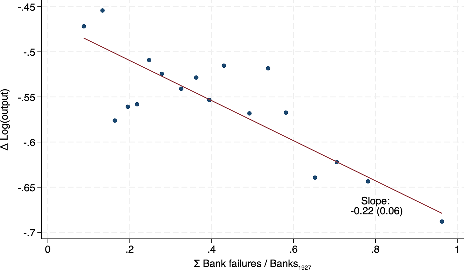


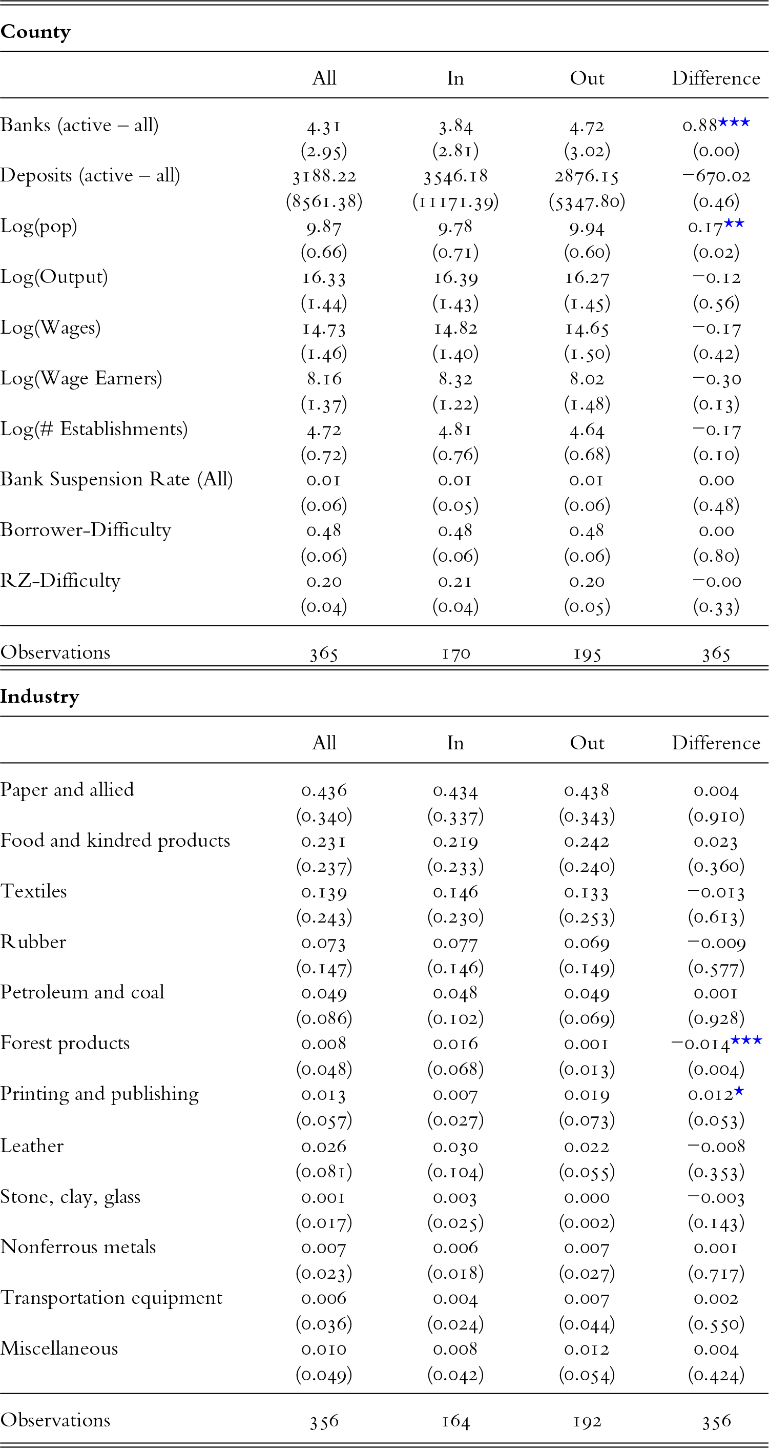

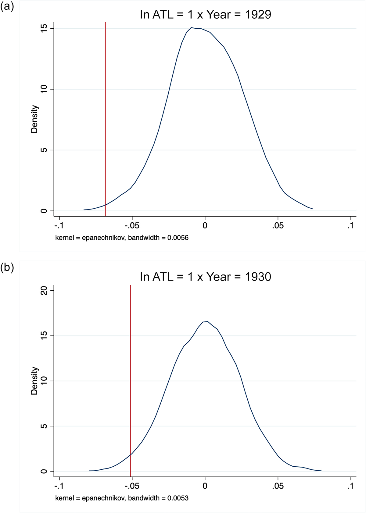
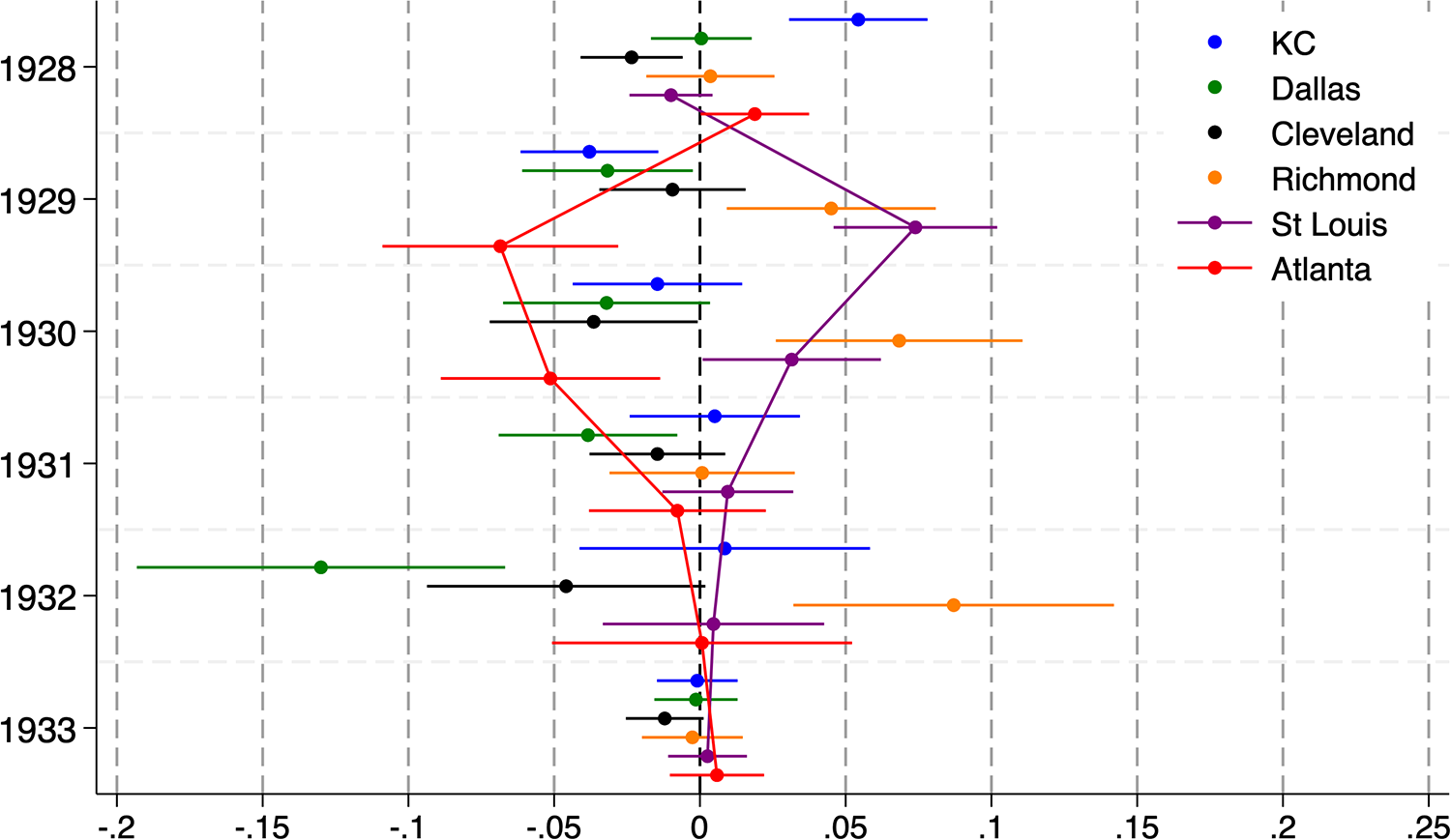
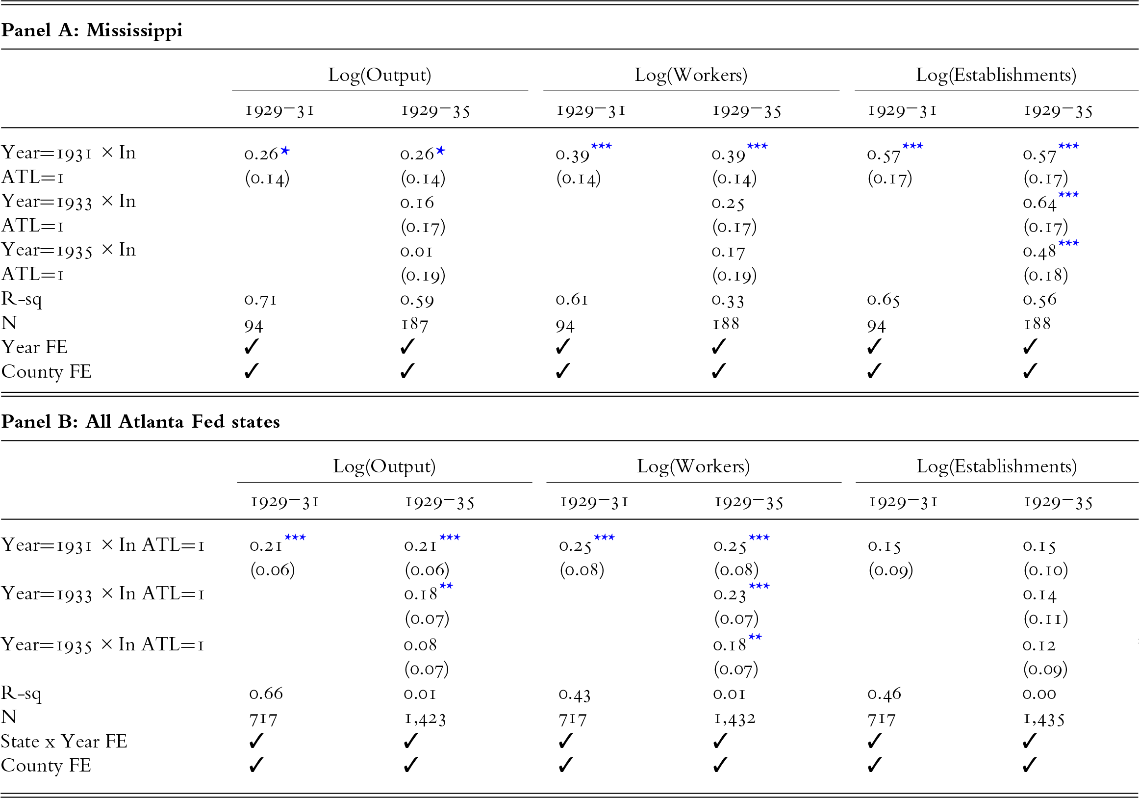
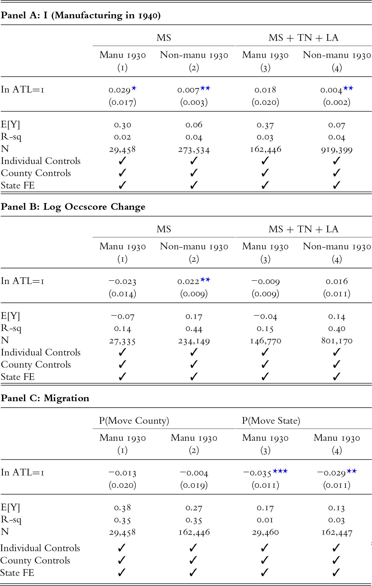


 Open access

