1 Introduction
In both civilian and military settings, effective management of airspace is an important and difficult problem. Air traffic controllers must cope with increasing volume and congestion around commercial airports when determining corridors and sequences for landing, takeoff and holding. Air campaign planners must synchronize large numbers of concurrent missions within a limited theater airspace, to be executed using diverse and increasingly autonomous sets of air vehicles. The key challenge in both cases is to ensure appropriate separation between all vehicles at all times, and to do so without significantly degrading the efficiency of individual movements. Viewed another way, this challenge can be seen as the problem of efficiently allocating shared airspace to movements over time.
In this paper, we take the view of airspace deconfliction as an extended resource allocation problem, and consider the problem of planning and scheduling vehicle movements to satisfy spatial constraints in addition to time and capacity constraints. As a first step we propose an efficient, scalable representation of spatial constraints over time based on a linear octree. We then define an extended planning/scheduling algorithm that utilizes this representation to construct a conflict-free schedule for accomplishing a given set of movements with a given set of vehicles. The extended algorithm assumes the existence of a base algorithm for computing a resource-feasible solution to the problem, which is used to compute ‘spatial capacity’ profiles and identify subspaces of likely spatio-temporal contention. Similar to other contention-based scheduling strategies (Sadeh, Reference Sadeh1991; Smith, Reference Smith1994; Beck, Reference Beck1999; Cesta et al., Reference Cesta, Oddi and Smith2002), this profile is used to direct the search for conflict-resolving changes to movement itineraries and/or timing constraints.
Central to the computation of a conflict-free schedule is the definition of an airspace conflict. We explore two different notions. A fine-grained definition of airspace conflict is formulated first, based on the ‘closest point of approach’ (CPA) of the separation buffers associated with two vehicle trajectories. A vehicle's separation buffer is a surrounding spatio-temporal region (the size and shape of which are a function of the type of vehicle), which accounts for the positional uncertainty of the vehicle as it moves. Under this definition, a conflict-free schedule is one in which no two vehicle separation buffers ever intersect. However, given the uncertainty associated with air flight parameters and the evasive capabilities of onboard processes (either manual or automated), an alternative approach to determining movement plans and schedules that is aimed at giving more deconfliction autonomy to individual vehicles can provide a more robust execution framework. To this end, we propose a second, coarser-grained definition of conflict, based on the presence of >n vehicles within a given spatio-temporal neighborhood. This ‘neighborhood’ is determined using larger separation zones called encounter regions that are, like separation buffers, associated with each vehicle. For any spatio-temporal neighborhood containing i vehicles (2 ⩽ i ⩽ n), there is some possibility that real-time, evasive actions will be necessary to avoid collisions among the vehicles. Given this, we compute an encounter set for each aircraft that identifies all other aircraft to avoid, which can be communicated in addition to its scheduled itinerary.
The remainder of this paper is organized as follows. We first describe our linear octree approach to representing airspace capacity constraints over time, assuming a fine-grained definition of airspace conflict. Next we present an algorithm for constructing conflict-free movement schedules. To demonstrate the viability of our approach, we then describe results obtained by coupling our algorithm with a previously developed system for air campaign scheduling and using it to generate realistically sized air campaign schedules. Turning attention to the concept of an integrated planning and execution framework, we next develop and evaluate a dual octree representation based additionally on encounter regions, which enables the construction of movement plans and schedules with some tolerable level of conflict. We conclude with a discussion of some limitations of our current model and a description of our current research plans.
2 Managing airspace as a capacitated resource
The allocation of airspace to a large set of missions requires an efficient and scalable representation scheme. Airspace capacity, in the form of contiguous corridor-like 4D spatio-temporal regions, must be rapidly retrievable in response to extensive queries from the resource scheduler and must continue to be so as that capacity is depleted. To deliver this functionality, we make use of the octree, a hierarchical, spatial (i.e., 3D) data structure that recursively divides a spatial volume into smaller subspaces for storing objects according to [x,y,z] coordinates. Hierarchical data structures rely on the concept of recursive decomposition to repeatedly divide large heterogeneous spaces into smaller and more manageable homogeneous subspaces (see Samet (Reference Samet1990) and Gaede and Günther (Reference Gaede and Günther1998) for more general discussions of multidimensional storage mechanisms).
The use of hierarchical structures for representing multidimensional data has been employed across a broad range of problem domains, including image processing, computer graphics, geographical information systems and robotics (e.g., for collision detection). The octree is a natural data structure for representing spatial or geographic data, typically characterized by [longitude, latitude, altitude] triplets. An octree decomposes a 3D volume by recursively halving it along each of its three coordinate axes until each subspace (called an octant or voxel) achieves some domain-specific condition (e.g., commonality among, or threshold of objects) or cannot be further subdivided (i.e., owing to its having reached a minimal size). In our case, in accordance with our fine-grained conflict definition, an octant is subdivided when it registers a conflict between two or more vehicle routes within its spatio-temporal bounds, in which case the area where the conflict occurs will be localized into a single octant or a cluster of abutting octants, to enable easy access to that particular area of contention. The subdivision of octants in response to coarser-grained neighborhood conflicts is discussed in a later section.
To manage space as a capacitated resource using an octree, we begin by mapping the entire spatio-temporal environment through which vehicles will be traveling into a single large octant (the initial configuration of the octree). As mission routes are planned and scheduled, they are inserted into the octree to reflect their exclusive right to a portion of spatial capacity for a particular period of time. Each octant designates a 3D volume whose contents are the vehicle route segments that intersect its region at any point in time. Airspace capacity can only be allocated to a vehicle if there are no other vehicles traveling along the same route or intersecting it at any time. That is, all vehicles must remain spatio-temporally independent of one another, or conflict-free, along their entire routes. Sufficient capacity for a vehicle route is dependent on there being a 4D path through space and time that does not conflict with any other vehicle routes. To find capacity for a vehicle, the scheduler must query what is typically a sequence of contiguous octants intersected by each leg of its route to ensure that sufficient spatio-temporal capacity is available for the duration of the route.
In a tree representation of an octree, each octant (except for those at the leaf level), has eight children (i.e., 2n, where n is the number of dimensions being represented). Its overall structure can therefore become quite large and unwieldy as the number of octants increases, and the process of searching for a particular octant within the tree can become more costly. To avoid this problem, we represent the octree as a linear octree (Gargantini, Reference Gargantini1982). The idea behind a linear octree is to assign each octant in the octree a unique key derived from its 3D location (i.e., its origin) and then represent the octree as a balanced binary tree. This approach requires significantly fewer pointers, and the use of the keys facilitates rapid access to the octants. Given a key, its corresponding octant node can be located quickly (in O(log N) time, where N is the number of octants) using a fast binary search instead of by traversing the possibly extensive paths within a regular octree. The keys are generated by translating points in 3D space into binary x, y and z coordinates and then interleaving the resulting bits to derive an integer value (also called a Morton code (Morton, Reference Morton1966)).
2.1 Vector-based vehicle routes
To represent the continuous movement of a vehicle through airspace, we use a contiguous sequence of 4D vectors, ![\[--><$> \overrightarrow{{{{v}_i}}} {\rm{:}}\left[ {{\rm{\rDelta }}{{x}_i},{\rm{\rDelta }}{{y}_i},{\rm{\rDelta }}{{z}_i},{\rm{\rDelta }}{{t}_i}} \right] <$><[[](https://static.cambridge.org/binary/version/id/urn:cambridge.org:id:binary:20151128095935283-0214:S0269888912000239_eqnU1.gif?pub-status=live) , that connect a sequence of [x,y,z,t] waypoints. Vehicles travel at a constant speed, constrained by platform type, over the duration of each vector. Inside the octree, each vector
![\[--><$> \overrightarrow{{{{v}_i}}} <$><[[](https://static.cambridge.org/binary/version/id/urn:cambridge.org:id:binary:20151128095935283-0214:S0269888912000239_eqnU2.gif?pub-status=live) will intersect one or more spatially contiguous octants based on these waypoints and the vectors linking them. Each octant can be thought of as a bucket containing annotated pointers to all of the vectors that intersect it, with each annotation indicating the times when the vector enters into and exits from the octant.
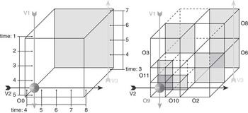
Figure 1 illustrates how an octree and its constituent octants organize an airspace volume and how vectors populate those octants. The left-hand side of the figure shows two intersecting vectors (![\[--><$> \overrightarrow{{{{v}_{\rm{1}}}}} <$><[[](https://static.cambridge.org/binary/version/id/urn:cambridge.org:id:binary:20151128095935283-0214:S0269888912000239_eqnU3.gif?pub-status=live) and
![\[--><$> \overrightarrow{{{{v}_{\rm{2}}}}} <$><[[](https://static.cambridge.org/binary/version/id/urn:cambridge.org:id:binary:20151128095935283-0214:S0269888912000239_eqnU4.gif?pub-status=live) ) and a third independent vector (
![\[--><$> \overrightarrow{{{{v}_{\rm{3}}}}} <$><[[](https://static.cambridge.org/binary/version/id/urn:cambridge.org:id:binary:20151128095935283-0214:S0269888912000239_eqnU5.gif?pub-status=live) ). Suppose the temporal extent of the three vectors (within the octree) is as follows:
![\[--><$> \overrightarrow{{{{v}_{\rm{1}}}}} [1 .\,. 5) <$><[[](https://static.cambridge.org/binary/version/id/urn:cambridge.org:id:binary:20151128095935283-0214:S0269888912000239_eqnU6.gif?pub-status=live) (i.e., a continuous temporal extent of 1 inclusive to 5 exclusive),
![\[--><$> \overrightarrow{{{{v}_{\rm{2}}}}} [4 .\,. 8) <$><[[](https://static.cambridge.org/binary/version/id/urn:cambridge.org:id:binary:20151128095935283-0214:S0269888912000239_eqnU7.gif?pub-status=live) and
![\[--><$> \overrightarrow{{{{v}_{\rm{3}}}}} [3 .\,. 7) <$><[[](https://static.cambridge.org/binary/version/id/urn:cambridge.org:id:binary:20151128095935283-0214:S0269888912000239_eqnU8.gif?pub-status=live) , and that the vectors represent vehicles traveling at the same speed. Recall that two or more vectors can reside in the same octant if they occupy non-overlapping intervals of time and space. A conflict occurs—indicating that capacity in a region is exceeded—when two or more vectors spatio-temporally intersect. In the figure, note that
![\[--><$> \overrightarrow{{{{v}_{\rm{1}}}}} <$><[[](https://static.cambridge.org/binary/version/id/urn:cambridge.org:id:binary:20151128095935283-0214:S0269888912000239_eqnU9.gif?pub-status=live) and
![\[--><$> \overrightarrow{{{{v}_{\rm{2}}}}} <$><[[](https://static.cambridge.org/binary/version/id/urn:cambridge.org:id:binary:20151128095935283-0214:S0269888912000239_eqnU10.gif?pub-status=live) intersect at an [x,y,z] coordinate in the near-lower-left corner of octant O 0 at time 4.5. If the temporal extent of
![\[--><$> \overrightarrow{{{{v}_{\rm{2}}}}} <$><[[](https://static.cambridge.org/binary/version/id/urn:cambridge.org:id:binary:20151128095935283-0214:S0269888912000239_eqnU11.gif?pub-status=live) was instead [1..5) (i.e., the same as
![\[--><$> \overrightarrow{{{{v}_{\rm{1}}}}} <$><[[](https://static.cambridge.org/binary/version/id/urn:cambridge.org:id:binary:20151128095935283-0214:S0269888912000239_eqnU12.gif?pub-status=live) ), then no conflict would occur, since the two vehicles traveling on those vectors would not be at the same [x,y,z] coordinate at any point in time.
Octant division in response to a conflict between two vectors ![\[--><$> \overrightarrow{{{{v}_{\rm{1}}}}} <$><[[](https://static.cambridge.org/binary/version/id/urn:cambridge.org:id:binary:20151128095935283-0214:S0269888912000239_eqnU13.gif?pub-status=live) and
![\[--><$> \overrightarrow{{{{v}_{\rm{2}}}}} <$><[[](https://static.cambridge.org/binary/version/id/urn:cambridge.org:id:binary:20151128095935283-0214:S0269888912000239_eqnU14.gif?pub-status=live) : before (l) and after (r); populated octants have shaded backs (red indicating a conflict), empty octants are not shown

In response to the introduction of the conflict between ![\[--><$> \overrightarrow{{{{v}_{\rm{1}}}}} <$><[[](https://static.cambridge.org/binary/version/id/urn:cambridge.org:id:binary:20151128095935283-0214:S0269888912000239_eqnU15.gif?pub-status=live) and
![\[--><$> \overrightarrow{{{{v}_{\rm{2}}}}} <$><[[](https://static.cambridge.org/binary/version/id/urn:cambridge.org:id:binary:20151128095935283-0214:S0269888912000239_eqnU16.gif?pub-status=live) , the octree will be subdivided twice, until (in this example), the octant containing the conflict reaches its minimal size, which is ideally set to be large enough to contain the conflict itself, but not much more than that. In the subdivision process, octant O 0 is first replaced by its eight children: octants O 1..O 8 (numbered from front-to-back, left-to-right, bottom-to-top, in the figure). The intermediate octant O 1 (in the near-lower-left corner) will subsequently be subdivided and replaced with octants O 9..O 16, leaving the conflict localized in octant O 9, where its contents can now be rapidly retrieved for the purposes of deconfliction. The resulting octree is shown on the right-hand side of Figure 1, with the vectors apportioned to octants as follows:
![\[--><$> \overrightarrow{{{{v}_{\rm{1}}}}} :[1 .\,. 3)\;{\rm{to}}\;{{O}_{\rm{3}}},\;\overrightarrow{{{{v}_{\rm{1}}}}} :[3 .\,. 4)\;{\rm{to}}\;{{O}_{{\rm{11}}}}\;{\rm{and}},\;\overrightarrow{{{{v}_{\rm{1}}}}} :[4 .\,. 5)\;{\rm{to}}\;{{O}_{\rm{9}}},\;\overrightarrow{{{{v}_{\rm{2}}}}} :<$><[[](https://static.cambridge.org/binary/version/id/urn:cambridge.org:id:binary:20151128095935283-0214:S0269888912000239_eqnU17.gif?pub-status=live)
![\[--><$>[4 .\,. 5)\;{\rm{to}}\;{{O}_{\rm{9}}},\;\overrightarrow{{{{v}_{\rm{2}}}}} :[5 .\,. 6)\;{\rm{to}}\;{{O}_{{\rm{10}}}}\;{\rm{and}}\,\overrightarrow{{{{v}_{\rm{2}}}}} :[6 .\,. 8)\;{\rm{to}}\;{{O}_{\rm{2}}} <$><[[](https://static.cambridge.org/binary/version/id/urn:cambridge.org:id:binary:20151128095935283-0214:S0269888912000239_eqnU18.gif?pub-status=live) , and finally
![\[--><$> \overrightarrow{{{{v}_{\rm{3}}}}} :[3 .\,. 5)\;{\rm{to}}\;{{O}_{\rm{6}}},\;{\rm{and}}\;\overrightarrow{{{{v}_{\rm{3}}}}} :<$><[[](https://static.cambridge.org/binary/version/id/urn:cambridge.org:id:binary:20151128095935283-0214:S0269888912000239_eqnU19.gif?pub-status=live)
![\[--><$>[5 .\,. 7)\;{\rm{to}}\;{{O}_{\rm{8}}} <$><[[](https://static.cambridge.org/binary/version/id/urn:cambridge.org:id:binary:20151128095935283-0214:S0269888912000239_eqnU20.gif?pub-status=live) . As long as conflicts do not occur, there is no limit on the number of vectors that can intersect and occupy an octant.
The process of querying the octree does not trigger any octant subdivisions, allowing the check for conflicts to be done as efficiently as possible. Assume that ![\[--><$> \overrightarrow{{{{v}_{\rm{1}}}}} <$><[[](https://static.cambridge.org/binary/version/id/urn:cambridge.org:id:binary:20151128095935283-0214:S0269888912000239_eqnU21.gif?pub-status=live) was inserted into the octree first. If the conflict between
![\[--><$> \overrightarrow{{{{v}_{\rm{1}}}}} <$><[[](https://static.cambridge.org/binary/version/id/urn:cambridge.org:id:binary:20151128095935283-0214:S0269888912000239_eqnU22.gif?pub-status=live) and
![\[--><$> \overrightarrow{{{{v}_{\rm{2}}}}} <$><[[](https://static.cambridge.org/binary/version/id/urn:cambridge.org:id:binary:20151128095935283-0214:S0269888912000239_eqnU23.gif?pub-status=live) had been detected before
![\[--><$> \overrightarrow{{{{v}_{\rm{2}}}}} <$><[[](https://static.cambridge.org/binary/version/id/urn:cambridge.org:id:binary:20151128095935283-0214:S0269888912000239_eqnU24.gif?pub-status=live) was inserted, by querying the octree to determine whether there was sufficient spatio-temporal capacity for
![\[--><$> \overrightarrow{{{{v}_{\rm{2}}}}} <$><[[](https://static.cambridge.org/binary/version/id/urn:cambridge.org:id:binary:20151128095935283-0214:S0269888912000239_eqnU25.gif?pub-status=live) 's route (i.e., in the original octant O 0), then the octant subdivision could have been avoided by either leaving
![\[--><$> \overrightarrow{{{{v}_{\rm{2}}}}} <$><[[](https://static.cambridge.org/binary/version/id/urn:cambridge.org:id:binary:20151128095935283-0214:S0269888912000239_eqnU26.gif?pub-status=live) out of the octree or modifying it either spatially or temporally to prevent the conflict.
2.2 Conflict detection
The linear octree facilitates the rapid retrieval of spatial capacity buckets that correspond to [x,y,z] coordinate locations. Given a route vector ![\[--><$> \overrightarrow{v} <$><[[](https://static.cambridge.org/binary/version/id/urn:cambridge.org:id:binary:20151128095935283-0214:S0269888912000239_eqnU27.gif?pub-status=live) starting at waypoint
![\[--><$> {{w}_1}:[{{x}_1},{{y}_1},{{z}_1},{{t}_1}] <$><[[](https://static.cambridge.org/binary/version/id/urn:cambridge.org:id:binary:20151128095935283-0214:S0269888912000239_eqnU28.gif?pub-status=live) and ending at waypoint
![\[--><$> {{w}_n}:[{{x}_n},{{y}_n},{{z}_n},{{t}_n}] <$><[[](https://static.cambridge.org/binary/version/id/urn:cambridge.org:id:binary:20151128095935283-0214:S0269888912000239_eqnU29.gif?pub-status=live) , the process of determining whether there is sufficient capacity for
![\[--><$> \overrightarrow{v} <$><[[](https://static.cambridge.org/binary/version/id/urn:cambridge.org:id:binary:20151128095935283-0214:S0269888912000239_eqnU30.gif?pub-status=live) begins by accessing the octant that contains w 1, interpolating the point
![\[--><$> {{w}_1}^\prime <$><[[](https://static.cambridge.org/binary/version/id/urn:cambridge.org:id:binary:20151128095935283-0214:S0269888912000239_eqnU31.gif?pub-status=live) at which it exits from the octant (if it does so), and then looking for spatio-temporal conflicts between the vector that contains the segment connecting w 1 and
![\[--><$> {{w}_1}^\prime <$><[[](https://static.cambridge.org/binary/version/id/urn:cambridge.org:id:binary:20151128095935283-0214:S0269888912000239_eqnU32.gif?pub-status=live) and other vectors with segments that occupy the same or directly abutting octant(s). This process continues with the remaining portion of the vector that extends past the bounds of the octant (i.e., from
![\[--><$> {{w}_1} ^\prime<$><[[](https://static.cambridge.org/binary/version/id/urn:cambridge.org:id:binary:20151128095935283-0214:S0269888912000239_eqnU33.gif?pub-status=live) to wn), and all subsequent vectors comprising a vehicle's route.
Determining whether a spatio-temporal conflict exists between two vectors involves more than just checking to see whether they intersect in four dimensions. A conflict condition between two vehicles actually occurs during any period of time when they are traveling too close to one another, because each vehicle has its own constant separation buffer (or maneuver avoidance zone: see Ennis & Zhao, Reference Ennis and Zhao2004) that designates a cylindrical spatial region centered on the vehicle (i.e., like a hockey puck), with which no other vehicle's own separation buffer may overlap. Separation buffers help account for the uncertainty inherent in the movement of vehicles over time: given the individual characteristics of a vehicle, its true location at any point in time may have strayed from its intended [x,y,z] position. Exclusion of other vehicles from the separation buffer zone ensures that each vehicle can travel safely within its own protective envelope.
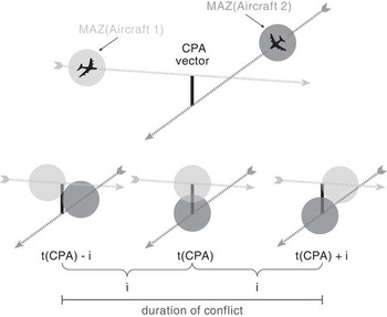
Detecting the overlap of vehicle separation buffers begins with the calculation of the CPA between their corresponding route vectors. Assuming that vehicles travel at a constant speed along a straight-line vector, a CPA calculation can identify both the exact point in time when two vehicles, traveling along two different vectors at possibly different speeds and times, will be closest to one another, and exactly what that distance will be. From there, it is possible to determine the temporal extent of any conflict, based on the sizes of their respective separation buffers.
This concept is illustrated in Figure 2. Two aircraft are set to cross paths. Their CPA, occurring at time t CPA, is described by the vector ‘CPA vector’. Using this vector (when there is a conflict), it is also possible to determine the points at which the separation buffers of the two aircraft are just about to overlap and just about to separate, which occurs some offset unit of time (i, in the figure) before and after t CPA. The temporal extent of the entire conflict is therefore ![\[--><$> [({{t}_{{\rm{CPA}}}}\,{\rm{ - }}\,i) .\,. ({{t}_{{\rm{CPA}}}}\, + \,i)] <$><[[](https://static.cambridge.org/binary/version/id/urn:cambridge.org:id:binary:20151128095935283-0214:S0269888912000239_eqnU34.gif?pub-status=live) .
Determining the overlap of vehicle separation buffers using a closest point of approach calculation. CPA = closest point of approach

2.3 Search among neighboring octants
Conflict detection is performed whenever a vector is considered for insertion into an octant, at which point its potential interaction with any vectors currently residing in the octant must be evaluated. An important issue when working with separation buffers—instead of simple vectors—is the need to perform conflict detection across octant boundaries, since overlap can occur between vehicles in adjoining, or neighboring octants. As a result, we have extended the conflict-detection mechanism to consider the vectors in neighboring octants as additional candidates for overlap whenever a vehicle is close enough to an octant boundary that its separation buffer could intersect with the separation buffer of a vehicle in an adjoining octant. Conveniently, the linear octree structure facilitates rapid access to neighboring octants (using their Morton codes), so access to such vehicle vectors is easily achieved, thereby enabling the conflict-detection process to consider all potential candidates for interference.
3 Conflict-free generation of movement schedules
Building on the representational techniques described in the previous section, we have developed an algorithm for generating conflict-free schedules in space and time (an earlier version of which is described in Hildum & Smith, Reference Hildum and Smith2007). Previous research with resource-constrained problems has emphasized the utility of access to resource contention profiles to inform look-ahead analysis techniques in the scheduling process (Sadeh, Reference Sadeh1991; Smith, Reference Smith1994; Beck, Reference Beck1999; Cesta et al., Reference Cesta, Oddi and Smith2002). The linear octree mechanism facilitates the generation of a similar assessment of the spatial resource requirements for a particular problem. Taking this approach, our algorithm utilizes an initial priming scheduling run performed ahead of the main scheduling phase, to populate the octree with all expected missions and identify all anticipated spatio-temporal areas of contention. This resource capacity profile is then used to guide the construction of a spatially conflict-free schedule during the second primary scheduling run.
During the first phase of the algorithm, the priming run generates a schedule that ignores spatial capacity constraints. Routes are built without any consideration for their interaction with one another, and in the process, a primed octree is populated, which localizes and highlights anticipated areas of contention for the entire problem, based on vehicle separation constraints.
During the primary (second) scheduling phase, the actual conflict-free schedule is built, and in the process, spatial capacity constraints are given the full attention of the scheduling algorithm. The route planner consults the previously constructed primed octree—now serving as an oracle—and modifies routes as necessary to avoid the conflicts with other vehicle routes appearing in the primed octree. The route-modifying operator attempts to introduce a horizontally displaced passing lane around each conflict, running parallel to the original vector. More intuitively, the route modifier tries to shift the conflicted portion of a route away from a conflict region within a conflicted octant, or from one conflicted octant to a less-conflicted neighboring octant. The efficiency of the linear octree representation again plays an important role here, enabling rapid access to the conflicted regions traversed by the route as well as the various neighboring octants to which conflicted traffic might be divertedFootnote 1.
3.1 The air campaign scheduling problem
To demonstrate our approach to conflict-free airspace scheduling, we consider a previously investigated air campaign scheduling domain (Myers et al., Reference Myers, Smith, Hildum, Jarvis and de Lacaze2001; Zhou & Smith, Reference Zhou and Smith2002). The general air campaign scheduling problem involves the allocation of aircraft and munitions to air strike missions over time in a battlefield domain. The problem has two broad types of inputs:
1. A set of targets for which individual air strike missions (sorties) must be scheduled. Each target has an associated target type, location and priority. For our purposes in this paper, we assume that each sortie can destroy a single target. Each target also has a specified time-on-target window during which it must be struck.
2. A description of resource capabilities, specifying (1) what types and amounts of resource capacity (aircraft, munitions, runways) are available for use, (2) where said resources are positioned in theater and (3) a table of weaponeering solutions that maps feasible aircraft/munitions pairs to target types.
The desired output is a schedule indicating the set of sorties to be flown. For each sortie, an aircraft and munitions quantity are allocated for a period of time allowing the target to be struck within its desired window, and a pair of takeoff and landing runway slots are reserved. The precise routes to be flown by each sortie are determined by our conflict-free scheduling algorithm.
3.2 Conflict-free air campaign scheduling
Our algorithm for generating conflict-free air campaign schedules builds on a previously developed ordered depth-first search procedure for incrementally generating air campaign and logistics schedules (Myers et al., Reference Myers, Smith, Hildum, Jarvis and de Lacaze2001; Zhou & Smith, Reference Zhou and Smith2002; Smith et al., Reference Smith, Becker and Kramer2004). Our extension augments this approach by taking resource-feasible vehicle missions that guarantee sufficient resource capacity over time (i.e., aircraft, munitions and runway access) and developing conflict-free routes for the aircraft to follow throughout the airspace.
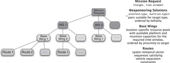
An illustration of the search schema employed to schedule an individual mission request is presented in Figure 3. To satisfy a mission request to strike a particular target within a desired time window, the scheduler first selects the most effective weaponeering solution for the target from among the set of feasible options. A weaponeering solution specifies a <platform-type, munitions-type> pair. Once the weaponeering solution is established, the next step is to determine the base wing from which the mission will be sourced. A base wing provides quantities of different platform types (e.g., kinds of aircraft) and associated munitions, as well as runway capacity for takeoffs and landings. There may be several candidate base wings that can provide a specific weaponeering solution. The list of suitable base wings is ordered by proximity to the target. If one base wing does not have enough available platform and munitions capacity at the desired time to satisfy the mission request, the next-closest base wing to the target will be explored.
The ordered depth-first mission-scheduling search schema. WS = weaponeering solutions

We expand this basic mission scheduling procedure by adding the lowest ply shown in Figure 3 to include the selection of a route for the mission, allowing it to traverse through the airspace to reach its target and return to the designated base wing from which it was sourced. Each route consists of a sequence of five contiguous flight vectors (i.e., ascent, approach, fly-by, return and descent)Footnote 2. The route is assembled after a base wing has been selected, and a platform, munitions and runway slots have been allocated to the mission. When a route is being assembled, spatial capacity constraints may or may not be enforced to ensure that the route avoids conflicts with other existing scheduled routes, depending on the top-level scheduling mode (see below). If the spatial capacity constraints are enforced, attempts are made to adjust an initially conflicted route both temporally (by shifting the mission downstream) and spatially (by altering the route to fly around a conflict). If these attempts fail to resolve all conflicts, the algorithm will backtrack and consider a different base wing or a different weaponeering solution. If all possibilities are exhausted, the mission request is abandoned.
The complete air campaign schedule is built incrementally by iteratively applying the search schema of Figure 3 to each input mission request. Missions are ordered according to the priority of their target, and preemption or any modification of existing scheduled missions is not permitted.
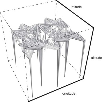
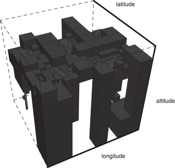
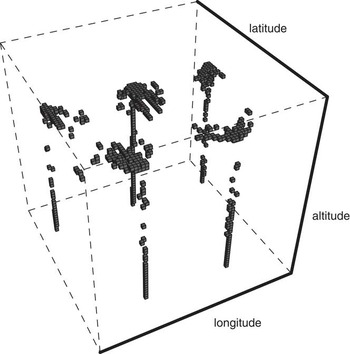
To illustrate the two-phase scheduling process, consider the 3D plot of 1000 air missions shown in Figure 4. These missions are sourced from a group of 10 bases to reach destinations in the center of the environment. The octants of a primed octree that contains these missions, generated during a priming run when spatial constraints are ignored, are shown in Figure 5. Blue/gray octants designate areas that contain one or more fully deconflicted air routes. The small red conflicted octants of Figure 5, which indicate the specific areas of contention, are isolated and shown in Figure 6. Octants with no traffic are not shown. All conflicts in the red octants must be resolved to achieve a fully deconflicted solution. The information contained in these octants is available during the subsequent primary scheduling phase to inform the route-planning component.
Flight paths for 1000 aircraft missions; colors are assigned randomly to distinguish between missions

Octants in a primed octree resulting from a priming scheduling run for 1000 aircraft missions; red octants indicate airspace regions containing vehicle conflicts, blue/gray octants indicate airspace regions free of any conflicts; empty octants are not shown

Conflicted octants from the plot in Figure 5

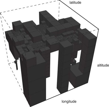
A final octree produced by the scheduling phase of the algorithm, when all spatial constraints are enforced to produce a conflict-free result, is illustrated in Figure 7Footnote 3. The absence of conflicted octants reflects the fact that all original conflicts from the priming run have been resolved through modifications to their routes.
Octants resulting from the primary scheduling phase for 1000 aircraft missions; the conflicts in all previously conflicted octants have been resolved through route modifications

3.3 Experimental results for conflict-free scheduling
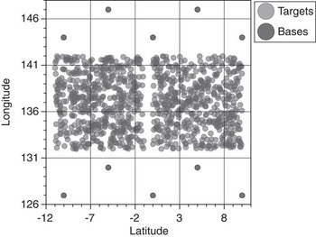
To evaluate the performance of our algorithm, we constructed a series of 20 data sets containing from 50 to 1000 randomly generated targets (in 50-target increments) spread across two roughly 700-miles-square adjoining regions, bracketed by 10 bases from which missions can be sourced. Each base is equipped with a complete cross-section and supply of the usable aircraft and munitions (and two runways), and each target is classified by one of 58 target categories that maps it to a set of feasible aircraft/munition pairs. All targets must be struck within a two-day time window. Figure 8 illustrates the largest, 1000-target data set and the common base locations for the entire series.
Evaluation data series: target and base layout (1000 targets, 10 bases)

In our evaluation, we compare the performance of our profile-based algorithm against a baseline approach that minimally extends the algorithm implemented by the underlying scheduling engine. These two approaches behave as follows:
• Baseline: As implemented by the underlying scheduling engine, the process of scheduling a sortie is a multi-tiered search process that at its highest level considers all feasible weaponeering solutions for the target, and then for each weaponeering solution, all bases equipped with its specified aircraft/munitions pairs. For each weaponeering-solution/base pair, the attempt is made to secure the necessary aircraft, munitions and runway capacity. The baseline extension to this process adds a call to the route planner, which attempts to build a conflict-free route indicating sufficient spatial capacity. If conflicts between the new route and any scheduled routes are detected in the octree, a single attempt will be made to deconflict it by rerouting it around the conflicts. If that attempt fails, the route planner will signal a failure and the scheduling engine will continue its search looking for available aircraft, munitions and runway capacity at the current base, but farther downstream in time. If, however, a conflict-free route is obtained, it is returned and the sortie is scheduled. When the timeline for a weaponeering-solution/base pair is exhausted, another feasible base is explored. When all bases for the weaponeering solution are exhausted, another feasible weaponeering solution is explored. If this process fails to secure the necessary aircraft, munitions, runway and spatial capacity, the sortie is marked as unschedulable.
• Profile-based: In our profile-based approach, the underlying scheduling engine behaves nearly identically to the baseline approach, except that the scheduler is run an additional time as a preprocessing step to populate the primed octree. During the priming phase, as described earlier, the route planner builds routes as usual, but does not check them for conflicts. Instead, it simply returns the first route it builds for a sortie, and the sortie is scheduled and assigned that route. During the primary scheduling phase, however, the route planner, when searching for airspace capacity, checks for conflicts by searching through the primed octree, which maintains an up-to-date summary of the airspace contention profile that reflects the entire set of sorties, both scheduled and unscheduled. If a conflict-free route is obtained (ideally the one built during the priming phase), it is returned to the scheduler. If there are conflicts that can be resolved through route modification (i.e., relative to the primed octree), the modified route is returned. If a conflict-free route cannot be obtained, the route planner will again signal a failure, and the search process of the underlying scheduling engine will explore other feasible options (just as in the baseline case).
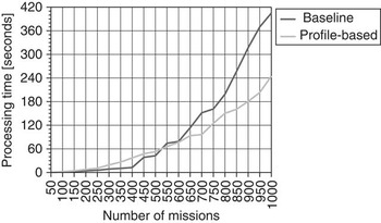
The performance results in Figure 9 show the amount of processing time required by each approach in scheduling the 20 random data sets. Note that both approaches are able to produce conflict-free schedules that include all of the missions in each of the data sets.
Comparison of processing times for baseline and profile-based scheduling approaches

These results emphasize an important point, which is that the additional overhead introduced by generating, maintaining and consulting a global spatial-contention profile (i.e., the primed octree populated with both scheduled and unscheduled sortie routes), is clearly compensated for by a notable improvement in overall scheduling performance for runs of more than a minute in duration (e.g., in excess of 500 missions). The ability of our profile-based approach to exploit the primed octree to resolve conflicts with both scheduled and unscheduled sorties earlier in the scheduling process makes it less likely that the eventual attempts to resolve them will be postponed until there are fewer resolution options available, and the cost of finding alternate solutions is greater.
4 Computing global movement plans with tolerable conflict potential
The use of conflict-free movement schedules such as those discussed in the previous section presumes a tight linkage between the airspace planner and executing air vehicles; whenever there is deviation from planned trajectories during execution, the global plan must be recomputed to ensure continued safe vehicle movement. Given the uncertainty associated with air movement, an alternative, and potentially more robust approach to global movement scheduling is to produce plans that assume some amount of autonomy on the part of individual aircraft to take appropriate deconfliction actions when necessary. In other words, global movement schedules can be constructed using a coarser notion of airspace conflict, which allows some specified amount of violation with respect to vehicle separation buffers. These coarser conflicts can be localized using a model of the spatio-temporal envelope needed by an aircraft to take evasive action during execution, and the set of aircraft that a given vehicle can be expected to encounter can be provided to the vehicle prior to execution to facilitate onboard deconfliction processes. In this section, we describe extensions of our basic approach to movement scheduling to support this kind of planning and execution framework.
4.1 Encounter regions
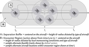
To support the generation of schedules with looser constraints on airspace conflicts, we expand the notion of the separation buffer zone by introducing the encounter region. This cylindrical region, which like the separation buffer is centered on the aircraft, provides an approximation of the larger region of uncertainty that surrounds an aircraft owing to the possibility that it may have to deviate from its nominal trajectory (e.g., change its speed or direction to avoid violating the separation buffer zone of another aircraft). Encounter regions are only utilized when an aircraft is placed in the position of having to perform its own autonomous deconfliction maneuvers, that is, when the aircraft's separation buffer zone intersects with the separation buffer, or ‘active’ encounter region, of another aircraft. During these times, the larger encounter region must be protected, and other aircraft must maintain separation from this larger region; otherwise, only the separation buffer zone need be honored.
The basic geometry of the encounter region is illustrated in Figure 10. The figure shows an aircraft traveling along a flight vector, viewed from above. The aircraft's separation buffer zone, labeled A, is centered on the aircraft with a width and height (not shown) specific to the aircraft type. The encounter region, labeled B, defines the larger volume that captures the wider set of feasible positions for an aircraft as it responds on its own to a potential conflict. Its dimensions are dictated by the individual capabilities of the aircraft and its current state (e.g., speed, heading, attitude).
Spatial geometry of the separation buffer zone and encounter region

The primary impact of reasoning about conflicts in terms of these two different kinds of aircraft separation constraint models is the need for dual octrees: one for enforcing the smaller separation buffer zones and one for enforcing the larger encounter regions. The details of this dual octree approach are described below.
4.2 Determining potential conflict
Encounter region intersections alone are not sufficient to indicate a potential conflict between aircraft. As mentioned above, encounter regions come into play when an aircraft maneuvers locally on its own in response to an expected separation buffer violation, thereby expanding the region of uncertainty surrounding its location for a period of time. The primary implication is that the process of determining whether an aircraft is involved in a potential conflict with another aircraft (i.e., whether their vectors intersect) must now employ different spatial constraints, depending on the conditions under which the aircraft—and any potential conflicting aircraft—are traveling at any point in time.
For this purpose, we use the term encounter mode to describe the situation when an aircraft is utilizing its larger encounter region to maneuver locally to avoid one or more potential separation buffer violations. A vehicle automatically switches into encounter mode whenever its separation buffer is violated. As soon as a separation buffer violation occurs, the minimum-distance constraints for determining what is a vector-to-vector conflict between two vehicles switch from those defining the smaller separation buffer to those defining the larger encounter region for each vehicle type. When a separation buffer violation ends, the minimum-distance constraints revert to normal.
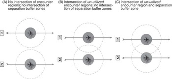
To clarify the use of these two regions in determining whether two vectors intersect, consider Figure 11. Three canonical non-conflict scenarios are displayed in this figure, based on varying degrees of intersection between the encounter regions and separation buffer zones of two aircraft. In case A, there is no intersection whatsoever between the two aircraft: their encounter regions are both not utilized, and do not intersect. By extension, their separation buffer zones also cannot intersect, so there is no possibility of conflict. In case B, while there is intersection between the two encounter regions, again not utilized, there is no intersection between the separation buffer zones, so there is no possibility of conflict. In case C, there is intersection between the encounter region of one aircraft and the separation buffer zone of the other aircraft, but again, because the encounter regions are not utilized (i.e., neither aircraft is operating in encounter mode) and there is no intersection between the separation buffer zones, there is no conflict.
Canonical non-conflict scenarios between vehicle pairs

Figure 12, conversely, displays three canonical scenarios of potential conflict between two vehicle route vectors. This time, in case A, there is an intersection between the encounter regions of both vehicles—utilized or not, and there is an intersection between the separation buffer zones as well. This case describes the most straightforward potential conflict scenario. Both aircraft will enter encounter mode, thereby utilizing their full encounter regions, and, in this situation (i.e., owing to the overlap in their encounter regions), route modifications will be required to ensure that their encounter regions are kept completely independent of one another for the duration of their loss of separation (LOS).
Canonical potential-conflict scenarios between vehicle pairs

Cases B and C in Figure 12 identify two special scenarios that can occur between intersecting aircraft routes, where at least one vehicle is operating in encounter mode, owing to interaction with some other vehicle. Case B shows an intersection between the encounter regions of two aircraft both operating in encounter mode (though unrelated to each other). Although there is no intersection between their separation buffer zones, the local maneuvering permitted while operating in encounter mode creates the potential for a conflict between the two aircraft, which may both be deviating from their nominal trajectories. Case C is a more specific example of the scenario in case B; in this situation, the utilized encounter region of one aircraft intersects with the separation buffer zone of the other aircraft, which may or may not be operating in encounter mode itself. Again, intersection with the separation buffer zone by a utilized encounter region leads to the potential for conflict between the two aircraft, and warrants route modifications to ensure that (1) at the very least, the encounter region of route 2 does not intersect with the separation buffer zone of route 1, and (2) in case route 1 is operating in encounter mode, the encounter regions of the two routes do not intersect.
4.3 Dual octree approach
To compute potential conflicts under the more flexible assumption of encounter region separation constraints, we adopt a dual octree representation. The dual octree approach works by populating two separate octrees with nearly duplicate mission data. The first octree enforces the separation constraints of the smaller separation buffers, while the second octree enforces the separation constraints dictated by the larger encounter regions. Because the encounter region octree allots each aircraft a wider area within which to maneuver, it registers a greater number of conflicts as contention levels increase within the airspace. Its attempt to provide each aircraft with a larger buffer between itself and all other aircraft is obviously more likely to fail. The separation buffer octree, conversely, grants each aircraft only its minimum necessary buffer, and as a result, allows for a much more tightly packed airspace by effectively increasing the threshold for signaling a conflict.
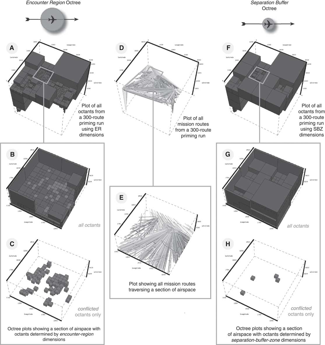
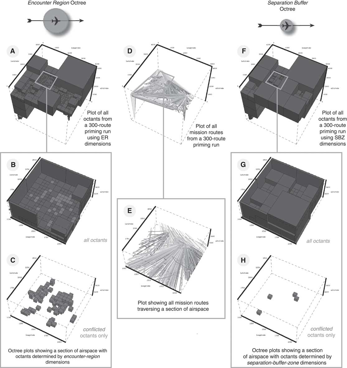
Figure 13 illustrates the dual-octree representation. On the left-hand side is a set of plots (labeled A, B and C) representing the larger encounter region octree (and portions of it) populated by a group of 300 air missions included in the center of the figure (labeled D). On the right-hand side is a set of plots (labeled F, G and H) representing the smaller separation buffer zone octree (and portions of it) populated by the same group of missions. Comparing the plots of the encounter region octree (A) and the separation buffer octree (F), it is evident that there are more conflicted octants in the encounter region octree, owing to the larger dimensions of the encounter regions, which lead to more vehicle conflicts. The close-up views into these octrees (B and G), and the companion plots showing only conflicted octants (C and H), highlight a particular spatial section of the airspace to further illustrate this point.
The dual-octree concept: the encounter region octree with wider separation constraints (left) signals more conflicts, while the separation buffer zone octree with narrower separation constraints (right) signals fewer, for the same set of missions. ER = encounter region; SBZ = separation buffer zone
The key to the dual octree approach is combining the constraint information maintained in each of the octrees to provide an accurate view of the actual contention within the airspace. By refining the view of contention obtained from the encounter region octree based on corresponding contention information from the separation buffer octree, we can determine the specific distance constraints to apply at any point to assess the severity of vector-to-vector conflicts based on the behavior of aircraft along their respective routes (i.e., whether or not either are in encounter mode). If a separation buffer zone is violated, then the larger encounter region must be enforced and honored for a period of time; otherwise, the continued protection of the separation buffer zones will suffice.
4.4 Conflict neighborhoods and encounter sets
As we mentioned earlier in the paper, the typical fine-grained definition of a conflict describes a scenario that involves, at the very least, two vehicles experiencing a loss of desired separation for a period of time. Our goal in this section is to specify and exploit a relaxed, coarser-grained definition of conflict that tolerates some amount of route intersection under the assumption that trajectories can be deconflicted by the aircraft involved at execution time. More precisely, we extend the notion of a conflict to refer more broadly to a collection of >n such intersecting routes. We refer to a spatio-temporal region where a set of >n routes intersect as a conflict neighborhood, and refer to n as the neighborhood size.
Under this extended definition of a ‘neighborhood’ conflict, the implication for the octree (i.e., both the encounter region octree and the separation buffer octree) is that an octant is not considered to be in conflict until it contains a single vector that intersects with ⩾n other vectors. As an example, consider a case when the neighborhood size is two. A pair of conflicting vectors will not signal a conflict in the octree, because each vector—within the octant that contains the intersection—only intersects with the one other vector. But if a third vector were to intersect with either of the other two vectors within the same octant, a conflict would be signaled, since all three vectors would be transitively linked by their intersections.
A second restriction imposed by the introduction of the conflict neighborhood is that a single route may not intersect with ⩾n other routes, which limits the number of aircraft that must deconflict themselves at execution time. It is important to note that a single vector can intersect with ⩾n other vectors in such a way that no single octant contains a single intersection of >n vectors. This would be the case, when n = 2, if a single vector of sufficient length is intersected by one vector at its start and with another vector at its end, leading to three intersecting routes, but possibly no single spatio-temporal region containing more than two intersecting vectors. As a result, it becomes necessary to perform additional checks, across octants, to ensure that the neighborhood sizing constraint is not violated in this way.
We call the set of all vectors with which a single vector intersects the encounter set for that vector. By extension, the encounter set for an aircraft route consisting of a sequence of vectors is the set of routes whose constituent vectors appear in the collected encounter sets of each of its vectors. The goal for the scheduler is to generate solutions in which there is no scheduled mission with an encounter set of a size that exceeds the neighborhood sizing constraint in effect.
Recall that an aircraft enters encounter mode whenever its separation buffer zone intersects with the separation buffer zone or the activated encounter region of another aircraft. When this occurs, its separation constraints expand to the size of the encounter region for the duration of the original separation buffer LOS, meaning that the aircraft may now be in conflict with a greater number of other aircraft than it otherwise would have been. To accurately assess the existence of conflict neighborhoods and construct encounter sets, the vector-to-vector intersection results from both octrees must be combined to determine exactly which losses of separation are significant.
The encounter set for a route is constructed by determining all instances where its vectors overlap spatio-temporally with other intersecting vectors because of a LOS between their separation buffers or activated encounter regions. And because encounter regions can be activated by interaction with other vectors that do not directly intersect with the route in question, it is necessary to propagate the spatio-temporal overlap across all related vector intersections (i.e., both direct and indirect) to assess the overall impact on a particular route.
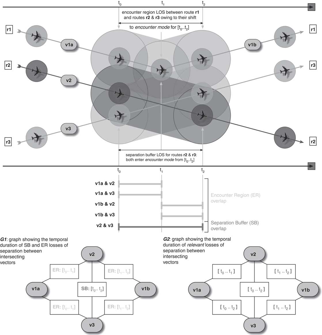
To illustrate this problem, consider the scenario presented in Figure 14. Routes r1 and r2 exist in the airspace. They fly together in parallel without any LOS between their separation buffers, and then diverge at time t 1. As a result, their encounter sets are both empty. But when a third route (r3) is added, it has a direct impact on r2, which leads to an indirect impact on r1. The LOS between the separation buffers of vectors v3 and v2 activates their encounter regions during the [t 0..t 2] temporal interval, which in turn causes a LOS between the encounter regions of v2 and vector v1a of r1 during [t 0..t 1] and v3 and vector v1b of r1 during [t 1..t 2]. The end result is that the insertion of r3 triggers a significant LOS between all three of the routes, resulting in an identical encounter set of {r1,r2,r3} for each one.
Problem scenario illustrating route vector overlaps and corresponding encounter set graphs
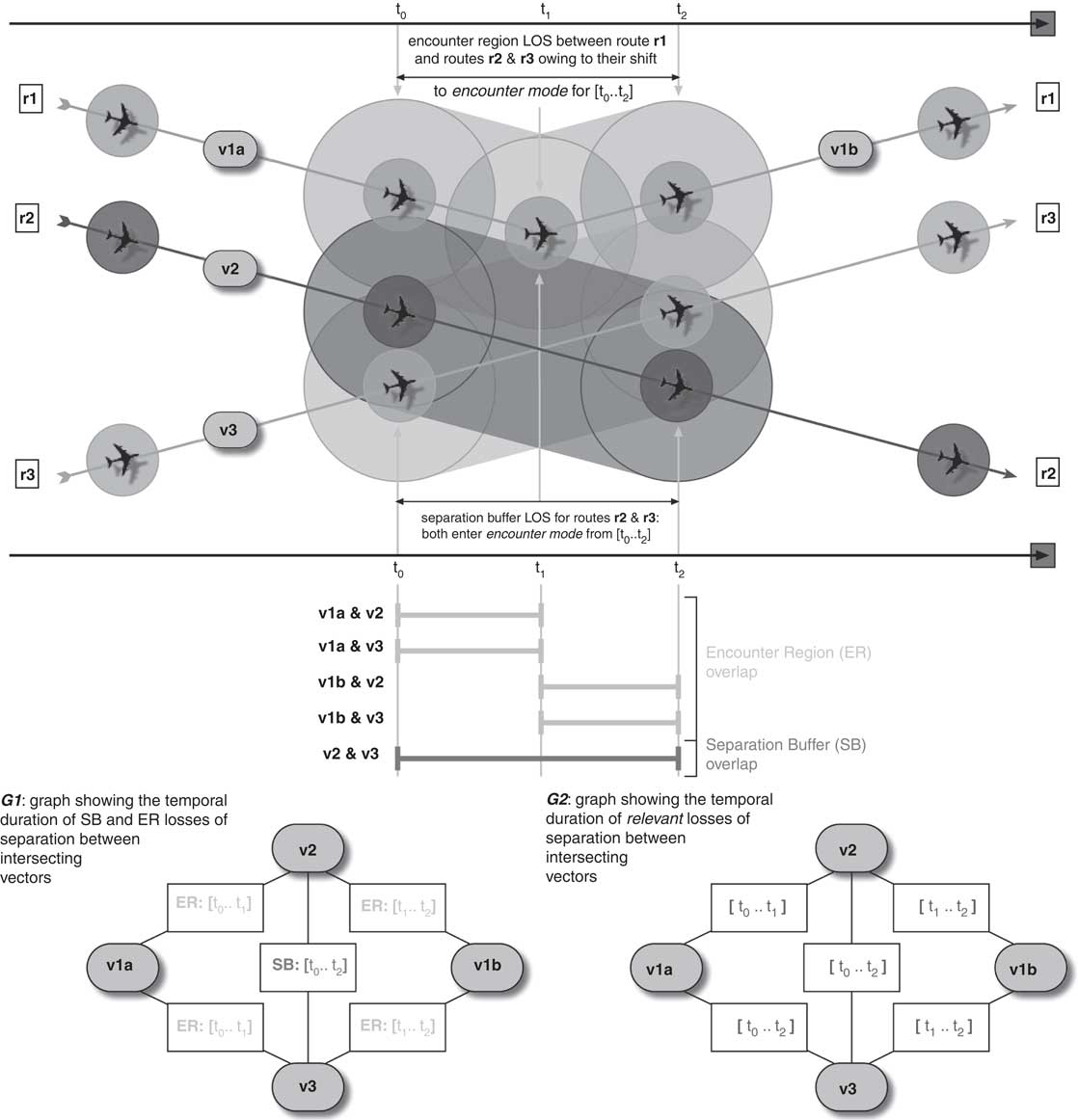
The process of determining encounter sets based on the spatio-temporal overlap of vectors is handled by a two-phase temporal propagation algorithm that produces two graphs (described below). Examples of these two graphs are provided at the bottom of Figure 14, labeled G1 and G2.
The first phase of this algorithm assembles a graph identifying the maximal overlap of LOS intervals among simultaneously intersecting vectors. Each pair of intersecting vectors is linked by an annotated arc recording the temporal bounds of the overlap and whether they result from a separation buffer or encounter region LOS. In graph G1 of Figure 14, note that v2 and v3 experience a separation buffer LOS during the interval [t 0..t 2] (the triggering LOS), v1a experiences an encounter region LOS during the interval [t 0..t 1] with both v2 and v3, and v1b experiences an encounter region LOS during the interval [t 1..t 2] with both v2 and v3.
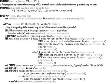
A high-level description of this phase of the algorithm is provided in Figure 15. It starts with a master list containing the vectors for a given route (or vehicle): [V 1, …, Vn] and a list of corresponding intervals initialized to their temporal extent. These intervals are used to propagate the bounds of simultaneous LOS intervals across chains of intersecting vectors to determine the maximal overlap for each vector. The algorithm proceeds by stepping through these lists in parallel using a breadth-first search.
High-level description of the closure algorithm for determining maximal temporal overlap of LOS intervals between vectors. LOS = loss of separation

On each iteration, the set of all vectors ![\[--><$> \{ I{{V}_{i,1}}, \ldots, I{{V}_{i,m}}\} <$><[[](https://static.cambridge.org/binary/version/id/urn:cambridge.org:id:binary:20151128095935283-0214:S0269888912000239_eqnU35.gif?pub-status=live) whose encounter regions intersect with that of the current Vi are retreived, and the bounds of their individual LOS with Vi are determined by tightening Vi's corresponding propagated bounds according to the bounds of the overlap between Vi and IVi ,j and the temporal extent of both vectors. In the case of a separation buffer LOS between Vi and IVi ,j, the bounds for that overlap are used instead of the bounds for the encounter region overlap, to more quickly tighten the propagated bounds and to identify guaranteed losses of separation. As soon as the propagated bounds are subsumed by any previously established bounds for the same vector, that branch of the search is pruned (because we are calculating the maximal overlap). Otherwise, each intersecting vector IVi ,j and its propagated bounds are added to the ends of the master lists for continued processing. The algorithm continues until the maximal temporal overlap among the transitive closure of simultaneously intersecting vectors reachable from the original [V 1, …, Vn] route vectors has been determined, which occurs when the propagated bounds have all been subsumed within the developing graph.
After this transitive closure vector-overlap graph has been produced, it is used to construct a new graph that identifies all separation buffer overlaps and those encounter region overlaps that involve encounter regions that have been activated by corresponding separation buffer overlaps. That is, it filters out any encounter region overlaps that involve encounter regions that are not activated by corresponding separation buffer overlaps, since those wider encounter regions are not actually being utilized by vehicles that are maneuvering to avoid separation buffer conflicts. An example of this relevant-overlap graph is labeled G2 in Figure 14. In this case, the LOS between the separation buffers of v2 and v3 activates their encounter regions during the temporal invterval [t 0..t 2], which reifies the previously identified encounter region overlaps between these vectors and both v1a and v1b, leaving them unchanged. The relevant temporal overlaps are recorded with the arcs.
This phase of the algorithm is described in Figure 16. The algorithm seeds a new master vector list with annotated entries corresponding to each arc in the vector-overlap graph (e.g., G1 of Figure 14) that represents a separation buffer LOS between two vectors. The algorithm proceeds in a fashion similar to that exhibited by the first phase of the algorithm. In this case, the process starts with the set of arcs representing separation buffer conflicts. For each arc, it propagates the bounds of its conflict outward to all of the connected vectors identified in the vector-overlap graph. Search branches are pruned once the propagated time bounds for a conflict are subsumed by any previuosly established temporal bounds for the same vectors. And as was the case before, these time bounds will tighten monotonically as they are propagated across overlapping vectors, ensuring that quiescense will be reached.
High-level description of the closure algorithm for propagating separation buffer overlap durations across the vector-overlap graph

Upon completion, the relevant-vector-overlap, or encounter set graph (e.g., G2 of Figure 14) identifies the set of vectors whose vehicles (1) experience a direct LOS with the separation buffer of another vehicle and (2) are forced into encounter mode to avoid the vectors of other locally maneuvering vehicles. By collecting the set of all vectors reachable from any particular vector in the graph, its encounter set can be determined, and by extension, the encounter set of its route. In Figure 14, the encounter set for all three routes is {r1,r2,r3}.
Using this two-phase temporal propagation algorithm, it is possible to construct a complete view of the impact of a proposed route on the set of all existing routes, to assess whether the neighborhood sizing constraint will be violated by the encounter set for the proposed route—or any existing route.
4.5 Experimental results for limiting conflict neighborhoods
In adopting this coarser-grained notion of conflict, the extended performance goal in generating air movement schedules is to ensure that any schedule generated for a set of air missions satisfies the neighborhood sizing constraint by limiting the size of any conflict neighborhood to n. To test this capability, we reused the data sets introduced earlier (see Figure 8) and added a new, second set of data sets that presented higher density movement problems. This time, the objective is to show that the neighborhood sizing constraints can be satisfied without imposing significant computational overhead.
We ran these data sets using a range of neighborhood sizing constraints appropriate to the level of contention within each respective data set. In the case of the original data sets used in Section 3.3, the largest conflict neighborhoods involved four conflicting aircraft, so the range of neighborhood sizes tested was [2..5]. The case where n = 5 serves as a kind of lower-bound benchmark since it requires no deconfliction effort on the part of the system. Obviously, a scheduling approach that allows coarser neighborhood conflicts solves a relaxed version of the problem; that is, it is acceptable to allow some degree of finer-grained conflicts between aircraft, and this requires less deconfliction effort on the part of the system. For the same reason, the tighter (i.e., lower in value) the neighborhood sizing constraint, the tougher it is to produce a ‘conflict-free’ solution. The second, higher-density version of the original data set was designed by eliminating half of the bases from which air missions could be sourced, meaning that all of the air traffic was focused to one side of the environment, thereby increasing the degree of contentionFootnote 4. In the higher density runs, the largest conflict neighborhoods involved seven aircraft, so the range of neighborhood sizes tested was [2..8].
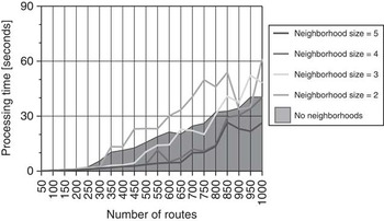
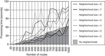
The results from the first set of experiments are shown in Figure 17, and the results from the high density experiments are shown in Figure 18. Note that in each set of results, when neighborhood sizing is turned on and the neighborhood size constraint is low (i.e., tight), the additional cost incurred to maintain and continually monitor all developing constraint neighborhoods pushes the processing times above those of the baseline case (where neighborhood sizing is turned off). Although the system is solving a relaxed version of the problem, there is a penalty paid for the necessary additional infrastructure and search effort. In the low-density results where there are fewer neighborhood conflicts to manage, the baseline performance is matched with a neighborhood size of three. In the high-density results, the baseline performance is matched with a neighborhood size of six. As the neighborhood size constraint value is increased (i.e., loosened), performance improves, and a crossover point is reached where the opportunity to solve a more relaxed version of the problem requiring less deconfliction compensates for the additional effort required to facilitate the conflict neighborhoods.
Comparison of processing times for various neighborhood sizes across a set of 20 data sets including from 50 to 1000 air missions

Comparison of processing times for various neighborhood sizes across a set of 20 higher density data sets including from 50 to 1000 air missions

In broad terms, these results confirm the utility of our dual octree approach for limiting the degree of conflict that exists among aircraft operating within a shared and potentially congested airspace, and demonstrate that these coarser-grained airspace deconfliction solutions can be generated with sufficient efficiency to provide flexibility to pilots and operators and preclude having to regenerate or significantly adjust an air campaign plan every time an aircraft deviates from its nominal course during execution.
5 Related work
Previous research in airspace deconfliction has focused primarily on the local problem faced by a particular movement activity (Stilman, Reference Stilman2000) or on dynamic real-time synchronization of multiple movements (OR Concepts Applied, 2002; Sridhar et al., Reference Sridhar, Chatterji, Grabbe and Sheth2002, Reference Sridhar, Sheth, Smith and Leber2005; Coppenbarger et al., Reference Coppenbarger, Lanier, Sweet and Dorsky2004). In both contexts, the principal goal is simply to make local planning and scheduling decisions that avoid airspace conflicts. The advantage of considering spatial constraints up front during more global planning and scheduling of a set of movements that must occupy a common airspace over a given time interval is that it provides the additional opportunity to optimize overall traffic flow by making efficient use of available airspace.
Other recent work has developed alternative techniques for representing and reasoning about 2D spatial constraints for purposes of detecting potential conflicts among surface movements that overlap in space and time (Yaman et al., Reference Yaman, Nau and Subrahmanian2005; Parker et al., Reference Parker, Yaman, Nau and Subrahmanian2007). The goal of this work, however, is to provide deductive machinery for answering queries relative to the space-time coordinates of known movements. The work described in this paper, in contrast, considers the larger problem of constructing a global movement plan and schedule that is conflict-free in 3D space and time and scalable to real-world problems.
Some current work in the management of air traffic in the civilian airspace employs a constraint programming solution to minimize the complexity of the problem by adjusting the numbers of flights admitted to established traffic sectors through the relaxation of takeoff times and the adjustment of en-route flight vectors (Flener et al., Reference Flener, Pearson, Agren, Garcia Vello, Celiktin and Dissing2007). This kind of approach is suitable for environments that enforce a strict pre-determined partitioning of airspace. Our work instead aims to avoid relying on such partitioning so that our conflict-free routing capabilities can yield greater efficiency of operations.
6 Summary
In this paper, we have considered the problem of constructing a movement plan for multiple vehicles that is conflict-free in space and time. By integrating spatial constraints directly into the planning and scheduling process, rather than considering airspace deconfliction after the fact from a local, tactical perspective, it is possible to anticipate likely areas of congestion and exploit opportunities to optimize traffic flow. Prior research has approached airspace deconfliction from a local, tactical perspective, and hence has focused rather exclusively on the more immediate problem of conflict avoidance.
Central to any approach to solving this extended resource allocation problem is a convenient, scalable basis for detecting airspace conflicts. To this end, we introduced a linear octree representation of available airspace capacity. We then used this octree representation to define a contention-driven scheduling procedure, wherein advance computation of a spatial capacity profile is used to direct the schedule generation process. Experiments performed using realistically sized problems from an air campaign planning domain showed this procedure capable of efficiently generating large-scale, conflict-free schedules, and for problems over a certain size, to outperform a simpler baseline procedure that instead utilized an octree representation without any look-ahead analysis.
To provide a more robust basis for integrating global movement scheduling with execution, we also investigated the use of a coarser-grained definition of conflict as a means of generating movement schedules that assume some amount of real-time, onboard deconfliction capability. We introduced the concept of an encounter region to delineate a larger spatio-temporal envelope within which a given air vehicle could execute its own evasive actions, and developed a dual octree representation that enables the generation of conflict neighborhoods of a limited size. Experiments using an extended set of air campaign problems showed the viability of this generalized movement scheduling procedure and its computational characteristics as the density of the vehicles in the airspace is varied.
7 Future work
One logical extension of our approach is to use a 4D hyper-octree representation of airspace, in which each octant designates a 4D spatio-temporal volume by treating the temporal dimension identically to spatial [x,y,z] dimensions. We are currently evaluating use of this extended representation, and our initial experiments suggest that significant speed-ups over the 3D implementation are possible.
Additional efforts are focused on three general research directions. First is the expansion of our spatial constraint model to encompass more diverse requirements. This includes adding support for:
• a wider range of vehicle types with different separation buffer volumes (we currently distinguish between fixed-wing and rotor aircraft types only) and different performance characteristics (e.g., unmanned aerial vehicles);
• weapons and other environmental threats (e.g., missiles, radar) that exhibit different spatio-temporal footprints, and may pop-up unexpectedly;
• special terrain features that constrain the route-planning and route-modification processes, either through inclusion (e.g., established or designated traffic corridors) or exclusion (e.g., high-threat, restricted or no-fly zones).
Second, we are working to enhance our route-building and modification techniques to reflect more sophisticated, real-world constraints on the maneuverability of mobile vehicles. Fuel availability strictly defines the range of feasible (re)routing options, while performance characteristics and other relevant flight variables limit the degree to which a vehicle's speed and trajectory can be altered in-flight. Additionally, we are exploring the opportunity to tailor route modification strategies to specific conflict scenarios, such as when one aircraft overtakes another along the same vector or when two aircraft are approaching one another head-on.
Finally, we are investigating the issues involved in translating movement plans into effective operational guidance for onboard deconfliction processes, and the ability to dynamically respond to the detected presence of unknown (and presumably uncooperative) vehicles within an evolving environment. Part of the process of developing a dynamic response capability involves the extension of the octree-based representation of available airspace over time to incorporate an aggregate model of airspace density. In its simplest implementation, density might be approximated by the number of air vehicles in a given region (or sector) of the airspace; more sophisticated measures could include such characteristics as the number of aircraft changing altitude, which tends to introduce greater complexity for humans in ensuring safe flight. The specification of an airspace density constraint for a particular region of the airspace could, in general, correspond to a set of contiguous octants in the octree (since octants are determined orthogonally during the process of localizing airspace conflicts). Our intention is to establish and manage these constraints dynamically, as a function of the set of missions and trajectories under consideration. With respect to the case of known (cooperative) manned mission trajectories, for example, we are looking to develop techniques for dynamically inferring manned flight regions from this data, and establishing different density constraints for allocating within and outside of these regions.
Acknowledgments
The work reported in this paper has been supported in part by the Boeing Company under contract CMU-BA-GTA-1-BOEING and the CMU Robotics Institute. The authors would like to thank Paul C. Parks and Patrick D. Hoy of the Boeing Company for sharing their expertise and providing valuable feedback and ideas about this work. Additionally, the authors are grateful to the reviewers for their insightful comments and suggestions with respect to earlier versions of this paper.