1. Introduction

In formal philosophy of science, certain simplifying and idealizing assumptions are often required in order to make questions tractable. The problem is that such assumptions can also get in the way, confounding results derived from our formal models. Results are confounded when they depend on a part of the model that does not accurately portray the target. Here is a simple toy example: even an ornate, highly detailed model of Cathédrale Notre-Dame de Paris will not represent every crack, patch, and cranny in the structure’s brick walls. To conclude from this model that the actual cathedral’s bricks are somewhat glossy and smooth would be a mistake; an idealized feature of the model will have confounded your “results” should you conclude this.

The nature of the idealizing assumption(s) made by one’s formal model naturally depends on the case. However, it is striking how often one particular idealizing assumption shows up (implicitly or explicitly) in formal philosophy of science, namely, the assumption that competing scientific hypotheses are mutually exclusive. This assumption is the subject of our article.

Many philosophers of science may not think of this as an idealizing assumption. They might think that this feature of a formal model gets the target right—at least often enough for it not to be a worrisome confounder. We accordingly argue in section 2 that competition is often not a simple matter of mutual exclusivity. If the mutual exclusivity assumption has an appropriate general place in formal philosophy of science, it is as a simplifying assumption allowing questions about competing hypotheses to be tractable, not as an accurate portrayal of reality. Highlighting the various ways in which consistent hypotheses may compete allows us to uncover two desiderata for a fuller and more accurate explication of hypothesis competition. In section 3, we use these two desiderata to motivate and defend a particular formal explication of hypothesis competition. In section 4, we use computer simulations and this formal explication to explore the extent to which, and conditions under which, this idealizing assumption can confound work in formal philosophy of science. We focus on the particular case of the study of Bayesian inference and its reliability. In section 5, we turn briefly to a case study to highlight further the need for a more careful treatment of hypothesis competition in the philosophy of science. We suggest that our explication provides the formal philosopher of science with a far more useful and accurate representation of what it takes for hypotheses to compete in actual scientific practice.

2. Desiderata for Hypothesis Competition

Competition between scientific hypotheses is very often not a matter of mutual exclusivity. It is easy to find actual cases of consistent scientific hypotheses being treated as competitors. There are two distinct ways in which consistent hypotheses may compete, each suggestive of senses in which a satisfactory account of hypothesis competition must part from the simple mutual exclusivity idea.

First, hypotheses that are not strictly speaking mutually exclusive may still do much to directly rebut each other; they may be logically consistent even if they nearly rule each other out. To give a simple example, a detective might judge it very unlikely that Smith and Jones carried out the robbery together because he knows they are sworn enemies. The upshot is that hypotheses may compete to varying degrees corresponding (at least in this case) to the extent that they disconfirm one another—how close they come to entirely ruling each other out. This gives rise to our first desideratum:

Second, hypotheses may compete with one another, even in cases in which they are not only consistent but perfectly compatible or even supportive of one another. There is no direct conflict between them in such a case, but they may nonetheless compete indirectly, via some body of evidence. Hypotheses compete in this way to the extent that adopting either hypothesis undermines the support that the relevant body of evidence provides for the other.

As an illustration of this from science, consider the ongoing debates about the mass extinction at the Cretaceous-Paleogene (K-Pg) boundary that brought an end to the dinosaurs around 66 million years ago. The leading hypothesis is the occurrence at this time in history of a bolide impact (Alvarez et al. Reference Alvarez, Alvarez, Asaro and Michel1980; Schulte et al. Reference Schulte2010), but other contending hypotheses include massive volcanism, climate change, and sea level regression. Overall, a vast number of further hypotheses have been proposed (Benton Reference Benton1990). Cleland (Reference Cleland2002, Reference Cleland2011) argues that historical science proceeds by (i) the proliferation of rival hypotheses to explain a puzzling body of traces and (ii) a search for a ‘smoking gun’ to discriminate between them. Many scientists claim that evidence relating to the K-Pg boundary—including the iridium anomaly and the existence of impact ejecta such as shocked quartz and spherules, as well as the discovery of the Chicxulub crater on the Yucatan peninsula in Mexico (Hildebrand et al. Reference Hildebrand1991) and evidence that ejecta at K-Pg boundary sites show a distribution pattern related to the distance from the crater (Schulte et al. Reference Schulte2010)—provides a smoking gun for the impact hypothesis.

Without considering the indirect pathway to competition, one might legitimately be led to question whether any of these hypotheses are really rivals (or competitors) at all—as Cleland’s approach requires. Certainly there is no logical incompatibility between the hypotheses mentioned above; any philosopher of science who explicates competition simply as mutual exclusivity will not be accurately representing this feature of the scientific debate.Footnote ¹ But note that hypotheses such as impact and volcanism are also not plausibly thought of as direct competitors at all. It is much more reasonable to treat them as independent before any evidence is taken into account since plausibly they do little or nothing to rebut each other directly to any significant degree.Footnote ² Rather, insofar as there is competition between these hypotheses, it comes indirectly by way of the body of evidence for which they both individually claim to account.

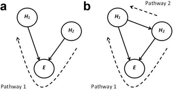
The upshot is that a full account of hypothesis competition needs to consider two different ways in which scientific hypotheses can compete. Figure 1 provides a visual representation of the two distinct “pathways to hypothesis competition.” Solid lines with arrows represent logical (deductive or inductive) relationships between propositions. In figure 1a, the absence of an arrow between H₁ and H₂ means that there is no direct support or disconfirming relation between these hypotheses. This means that H₁ and H₂ can only compete indirectly via E as indicated by pathway 1. In figure 1b, H₁ and H₂ have a direct bearing on one another, and so they may also compete directly if pathway 2 describes a disconfirming rather than supporting relation.

Figure 1.

a, H₁ and H₂ may only compete indirectly via pathway 1; b, H₁ and H₂ have the potential to compete directly via pathway 2 or indirectly via pathway 1.

The foregoing discussion gives rise to our second desideratum:

3. Direct and Indirect Competition

In Glass and Schupbach (Reference Glass and Schupbach2017), we develop and defend a formal explication of hypothesis competition that satisfies both of the above desiderata. In this section, we motivate the use of this measure explicitly in terms of direct and indirect pathways to competition, and we reiterate some important implications of competition explicated in this way.

Our explication is Bayesian only in the sense that it is probabilistic and uses the relevant probabilities as formal representations of rational degrees of belief (or credences) for a particular epistemic agent. Since these are probabilities, they are assumed to satisfy the standard Kolmogorov axioms; rational agent credences are thus at least synchronically coherent in our framework. Setting up our minimal Bayesian framework, if A is an algebra of propositions (including the tautology and closed under negation and disjunction), then probability function Pr: $A\to \left[0,1\right]$ assigns the degrees of belief that an ideal Bayesian agent has in any and all members of A. The degree to which one proposition (incrementally) confirms another is measured differently by distinct candidate measures. We favor the log-likelihood measure (and other measures ordinally equivalent to it). For any three propositions x, y, $z\in A$, this measure calculates the degree to which x confirms y, given z, as follows:

$C_l\left(x,y|z\right)=\log \left[\frac{\mathrm{Pr}\left(x|y\&z\right)}{\mathrm{Pr}\left(x|\neg y\&z\right)}\right]\mathrm{.}$

The degree to which proposition x disconfirms y, given z, is defined as the degree to which x confirms ¬y, given z:

$C_l\left(x,\neg y|z\right)=\log \left[\frac{\mathrm{Pr}\left(x|\neg y\&z\right)}{\mathrm{Pr}\left(x|y\&z\right)}\right]=-C_l\left(x,y|z\right)\mathrm{.}$

Using C₁, our measure of the overall (or “net”) degree to which H and H′ compete with respect to E may be represented as the average degree to which H and H′ disconfirm each other in light of E:

$\mathrm{Comp}\left(H,H^{\prime }/E\right)=\frac{C_l\left(H,\neg H^{\prime }|E\right)+C_l\left(H^{\prime },\neg H|E\right)}{2}\mathrm{.}$

Comp takes increasingly positive values to the extent that H and H′ compete (or disconfirm one another in light of E), decreasingly negative values to the extent that H and H′ support (or confirm) one another, and value 0 exactly when H and H′ are irrelevant to one another in light of E (this happens, e.g., when the direct and indirect competition or support between H and H′ with respect to E exactly cancel each other out).Footnote ³

We may demonstrate that Comp captures both pathways to competition by showing that it is a simple combination of separate measures of degree of direct and indirect competition respectively. Recall that competition between hypotheses H and H′ (where H, $H^{\prime }\in A$) occurs along the direct pathway to the extent that these hypotheses confirm the falsity of each other (i.e., “disconfirm” each other). In our previous paper, we used degree of disconfirmation $C_1\left(H^{\prime },\neg H\right)$ to represent the degree to which H′ directly rebuts H and used this as part of our account of competition. Here we extend this by using C₁ to formalize degree of direct competition Comp_D as the average degree to which either hypothesis confirms the negation of the other:

${\mathrm{Comp}}_D\left(H,H^{\prime }\right)=\frac{C_l\left(H^{\prime },\neg H\right)+C_l\left(H,\neg H^{\prime }\right)}{2}=\left(\log \left[\frac{\mathrm{Pr}\left(H^{\prime }|\neg H\right)}{\mathrm{Pr}\left(H^{\prime }|H\right)}\right]+\log \left[\frac{\mathrm{Pr}\left(H|\neg H^{\prime }\right)}{\mathrm{Pr}\left(H|H^{\prime }\right)}\right]\right)/2.$

Next, recall that competition between H and H′ occurs along the indirect path, by way of some body of evidence $E\in A$, to the extent that each hypothesis undermines the support that E provides for the other. To measure this extent, one must compare the degree to which E confirms either hypothesis (without consideration for the other hypothesis) with the degree to which E confirms that same hypothesis after the alternative hypothesis is accepted or assumed. For example, E confirms H to degree C₁(E,H); given H′, however, E confirms H to degree $C_1\left(E,H|H^{\prime }\right)$. In our previous paper, we defined the extent to which H′ turns E against H by subtracting the latter from the former: $C_1\left(E,H\right)-C_1\left(E,H|H^{\prime }\right)$. Here we use this approach to define the degree of indirect competition Comp_I as the average degree to which the hypotheses turn E against one another:

$\begin{array}{c}{\mathrm{Comp}}_I\left(H,H^{\prime }/E\right)=\frac{C_l\left(E,H\right)-C_l\left(E,H|H^{\prime }\right)+C_l\left(E,H^{\prime }\right)-C_l\left(E,H^{\prime }|H\right)}{2}\\ =\left(\log \left[\frac{\mathrm{Pr}\left(E|H\right)}{\mathrm{Pr}\left(E|\neg H\right)}\right]-\log \left[\frac{\mathrm{Pr}\left(E|H\&H^{\prime }\right)}{\mathrm{Pr}\left(E|\neg H\&H^{\prime }\right)}\right]+\log \left[\frac{\mathrm{Pr}\left(E|H^{\prime }\right)}{\mathrm{Pr}\left(E|\neg H^{\prime }\right)}\right]-\log \left[\frac{\mathrm{Pr}\left(E|H^{\prime }\&H\right)}{\mathrm{Pr}\left(E|\neg H^{\prime }\&H\right)}\right]\right)/2.\end{array}$

The desired result—that Comp captures both pathways to competition—then follows, as expressed in the following theorem:

Proof This follows from theorem 1 in Glass and Schupbach (Reference Glass and Schupbach2017).

$\begin{array}{c}{\mathrm{Comp}}_D\left(H,H^{\prime }\right)+{\mathrm{Comp}}_I\left(H,H^{\prime }/E\right)=(\log \left[\frac{\mathrm{Pr}\left(H^{\prime }|\neg H\right)}{\mathrm{Pr}\left(H^{\prime }|H\right)}\frac{\mathrm{Pr}\left(E|H\right)}{\mathrm{Pr}\left(E|\neg H\right)}\frac{\mathrm{Pr}\left(E|\neg H\&H^{\prime }\right)}{\mathrm{Pr}\left(E|H\&H^{\prime }\right)}\right]+\\ \log \left[\frac{\mathrm{Pr}\left(H|\neg H^{\prime }\right)}{\mathrm{Pr}\left(H|H^{\prime }\right)}\frac{\mathrm{Pr}\left(E|H^{\prime }\right)}{\mathrm{Pr}\left(E|\neg H^{\prime }\right)}\frac{\mathrm{Pr}\left(E|\neg H^{\prime }\&H\right)}{\mathrm{Pr}\left(E|H^{\prime }\&H\right)}\right])/2\\ =(\log \left[\frac{\mathrm{Pr}\left(H^{\prime }|\neg H\right)\mathrm{Pr}\left(E|\neg H\&H^{\prime }\right)}{\mathrm{Pr}\left(E|\neg H\right)}\frac{\mathrm{Pr}\left(E|H\right)}{\mathrm{Pr}\left(H^{\prime }|H\right)\mathrm{Pr}\left(E|H\&H^{\prime }\right)}\right]+\\ \log \left[\frac{\mathrm{Pr}\left(H|\neg H^{\prime }\right)\mathrm{Pr}\left(E|\neg H^{\prime }\&H\right)}{\mathrm{Pr}\left(E|\neg H^{\prime }\right)}\frac{\mathrm{Pr}\left(E|H^{\prime }\right)}{\mathrm{Pr}\left(H|H^{\prime }\right)\mathrm{Pr}\left(E|H^{\prime }\&H\right)}\right])/2\\ =\left(\log \left[\frac{\mathrm{Pr}\left(H^{\prime }|\neg H\&E\right)}{\mathrm{Pr}\left(H^{\prime }|H\&E\right)}\right]+\log \left[\frac{\mathrm{Pr}\left(H|\neg H^{\prime }\&E\right)}{\mathrm{Pr}\left(H|H^{\prime }\&E\right)}\right]\right)/2=\frac{C_l\left(H^{\prime },\neg H|E\right)+C_l\left(H,\neg H^{\prime }|E\right)}{2}=\mathrm{Comp}\left(H,H^{\prime }/E\right).\end{array}$

QED

Using our measure, we can make more precise sense of qualitative judgments of hypothesis competition. We explicate the judgment that H and H′ compete with respect to E (to some degree) as a positive degree of competition, $\mathrm{Comp}\left(H,H^{\prime }/E\right)>0$. Since positive degree of competition corresponds to the case in which H and H′ disconfirm one another in light of E (and ignoring cases in which Pr(H) or Pr(H′) is zero), we may also state the (qualitative) condition for competition using the following probabilistic inequality:

(1)$\begin{array}{}\mathrm{Pr}\left(H|H^{\prime }\&E\right)<\mathrm{Pr}\left(H|E\right)\mathrm{.}\end{array}$

In an earlier study on “explaining away,” Glass (Reference Glass, Chandler and Harrison2012, theorem 1) also proved that the following inequality provides another equivalent condition for competition:

(2)$\begin{array}{}\log \left[\frac{\mathrm{Pr}\left(E│H\&H^{\prime }\right)\times \mathrm{Pr}\left(E|\neg H\&\neg H^{\prime }\right)}{\mathrm{Pr}\left(E│H\&\neg H^{\prime }\right)\times \mathrm{Pr}\left(E|\neg H\&H^{\prime }\right)}\right]+\log \left[\frac{\mathrm{Pr}\left(H|H^{\prime }\right)\times \mathrm{Pr}\left(\neg H|\neg H^{\prime }\right)}{\mathrm{Pr}\left(H|\neg H^{\prime }\right)\times \mathrm{Pr}\left(\neg H|H^{\prime }\right)}\right]<0.\end{array}$

We can reapply (2) for our own purposes here, giving us another statement of the criterion for competition (to some degree). Equation (2) turns out to be especially useful insofar as it, unlike the other qualitative criteria, separates independent terms (the two summands) relating to the indirect and direct pathways by which competition can occur respectively.Footnote ⁴

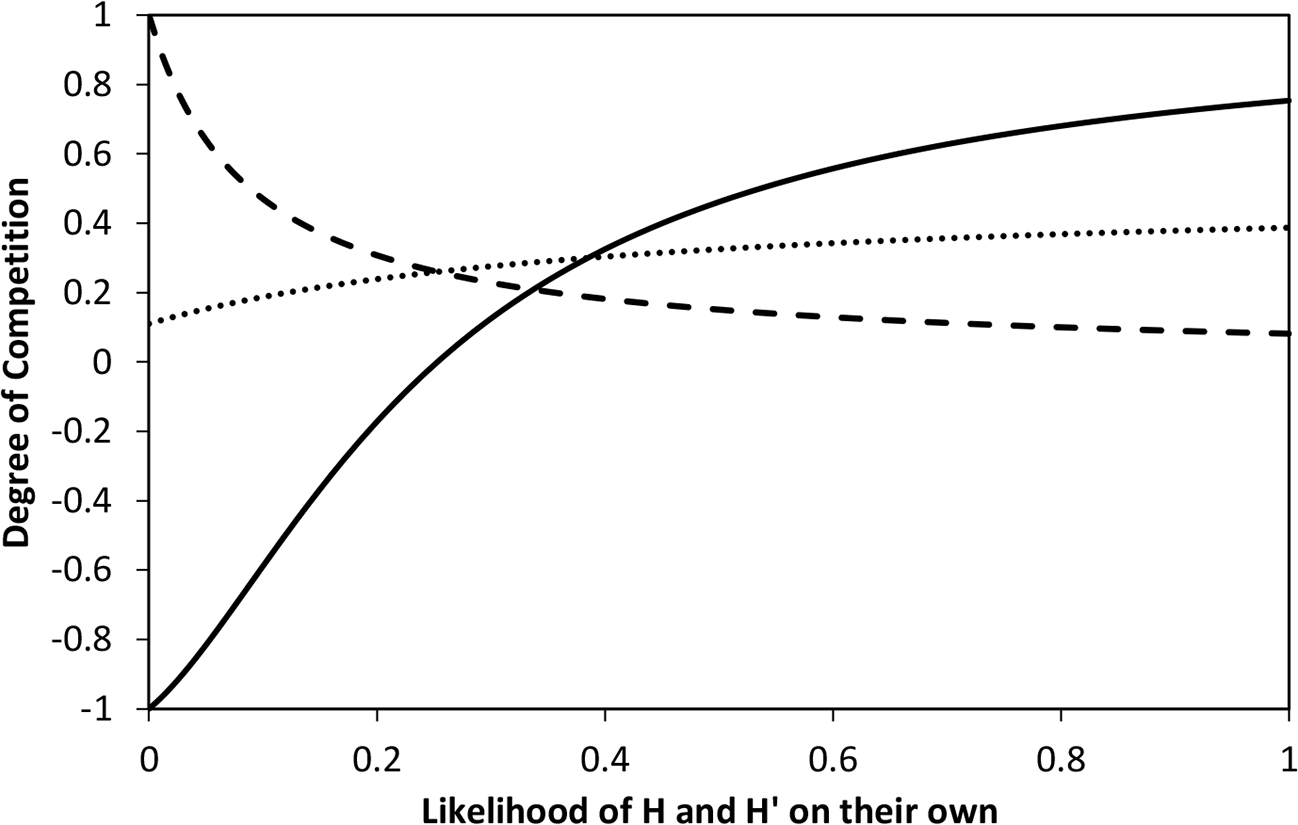
Figure 2 displays degree of competition as a function of the likelihoods for the hypotheses on their own (i.e., $\mathrm{Pr}\left(E|\neg H\&H^{\prime }\right)$ and $\mathrm{Pr}\left(E|H\&\neg H^{\prime }\right)$) in a scenario in which the hypotheses are independent before the evidence is taken into account, corresponding to the absence of direct competition as displayed in figure 1a, and to the case in which the second term in (2) is zero. The values of the probabilities $\mathrm{Pr}\left(H|E\right)$ and $\mathrm{Pr}\left(H|H^{\prime }\&E\right)$ are also shown in figure 2. For the limiting case in which the likelihoods are zero, the first term in (2) is infinite, and so the degree of competition is minimal. Essentially, this means that neither hypothesis can account for the evidence on its own since either hypothesis alone (i.e., conjoined with the negation of the other hypothesis) implies the falsity of E. Furthermore, when the likelihoods are zero, $\mathrm{Pr}\left(H|H^{\prime }\&E\right)=1$, and so given E, H′ guarantees the truth of H. As the likelihoods increase, so does the degree of competition until it reaches zero when $\mathrm{Pr}\left(H|H^{\prime }\&E\right)=\mathrm{Pr}\left(H|E\right)$, which occurs at a value of the likelihood close to 0.25. This corresponds to the first term in (2) being zero. For greater values of the likelihoods, $\mathrm{Pr}\left(H|H^{\prime }\&E\right)<\mathrm{Pr}\left(H|E\right)$, and so the degree of competition is positive. This corresponds to competition along pathway 1.

Figure 2.

Degree of competition (solid line) as a function of the likelihoods $\mathrm{Pr}\left(E|H\&\neg H^{\prime }\right)=\mathrm{Pr}\left(E|\neg H\&H^{\prime }\right)$, when $\mathrm{Pr}\left(H\right)=\mathrm{Pr}\left(H^{\prime }\right)=0.1$, $\mathrm{Pr}\left(E|H\&H^{\prime }\right)=0.8$, and $\mathrm{Pr}\left(E|\neg H\&\neg H^{\prime }\right)=0.08$. Also shown are $\mathrm{Pr}\left(H|H^{\prime }\&E\right)$ (dashed line) and $\mathrm{Pr}\left(H|E\right)$ (dotted line). Here we use an ordinally equivalent measure of competition with range [−1,1] (constructed using C_k as described in n. 3).

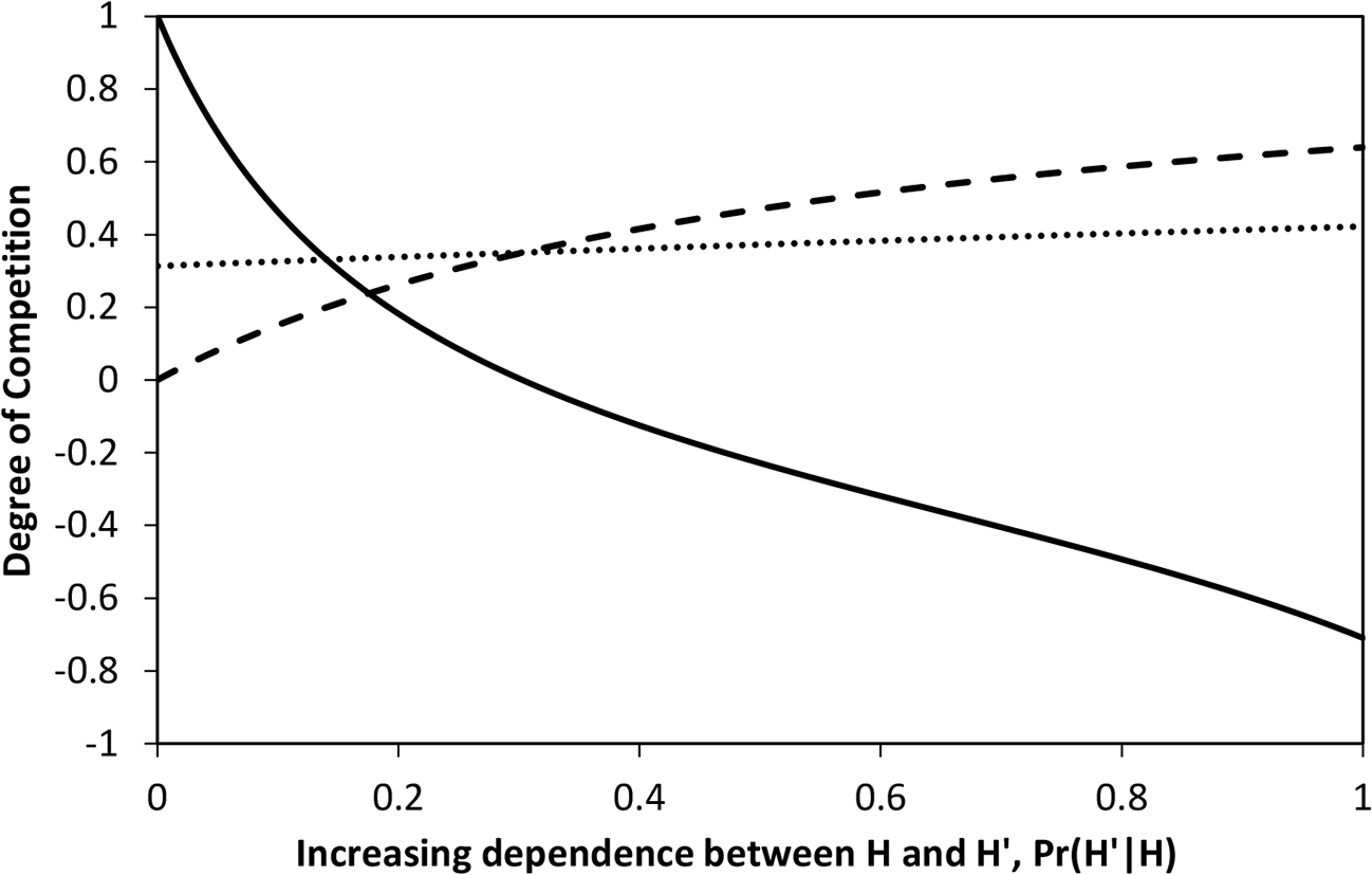
Figure 3 shows another scenario similar to the previous one but where there is a direct dependence between the hypotheses corresponding to figure 1b. Negative dependence between the hypotheses, which occurs for $\mathrm{Pr}\left(H^{\prime }|H\right)<0.1$, gives rise to competition via pathway 2 and so adds to the competition due to pathway 1. For sufficiently large positive dependence, the negative contribution via pathway 1 is cancelled out via the contribution from pathway 2 resulting in no competition. This occurs at$\mathrm{Pr}\left(H^{\prime }|H\right)=0.3$ when $\mathrm{Pr}\left(H|H^{\prime }\&E\right)=\mathrm{Pr}\left(H|E\right)$, and as the dependence between H′ and H increases further the degree of competition becomes lower still.

Figure 3.

Degree of competition (solid line) as a function of dependence between hypotheses: $\mathrm{Pr}\left(H^{\prime }|H\right)$ varies from 0 to 1, while $\mathrm{Pr}\left(H^{\prime }|\neg H\right)$ is fixed at 0.1; thus, dependence is negative for $\mathrm{Pr}\left(H^{\prime }|H\right)<0.1$ and positive for $\mathrm{Pr}\left(H^{\prime }|H\right)>0.1$. Apart from Pr(H′), other probabilities are as defined in figure 2 except that now $\mathrm{Pr}\left(E|H\&\neg H^{\prime }\right)$ and $\mathrm{Pr}\left(E|\neg H\&H^{\prime }\right)$ are fixed at 0.5. Also shown are $\mathrm{Pr}\left(H|H^{\prime }\&E\right)$ (dashed line) and $\mathrm{Pr}\left(H|E\right)$ (dotted line). Here we use an ordinally equivalent measure of competition with range [−1,1] (constructed using C_k as described in n. 3).

4. Computer Simulations of Bayesian Inference

In section 2, we argued that the mutual exclusivity assumption, although common in formal philosophy of science research, is often not true to scientific practice (the object of philosophy of science research). At best then, this assumption is a relatively innocuous idealizing assumption. At worst, it perniciously confounds a wide swath of work in contemporary philosophy of science. In this section, we present some initial research into the important questions of just how harmful this idealizing assumption can be to formal results and under what conditions.

In order to investigate the impact of incorrectly assuming that hypotheses are mutually exclusive on making inferences, we carried out computer simulations. The idea is first to define a probability model, which we will stipulate as the correct model, Pr, involving H, H′, and E, where H and H′ are not assumed to be mutually exclusive. We then modify this model to obtain what we will call the mutually exclusive probability model, Pr_X, where H and H′ are treated as mutually exclusive. The next step is to make inferences using the mutually exclusive model and determine how good they are by comparing them with inferences made using the correct model. Inferences are made by selecting the most probable hypothesis given E, so essentially we evaluate the mutually exclusive model by determining how often it identifies the same hypothesis as the correct model—or how often it correctly identifies the most probable of potentially competing hypotheses. Here we focus on how the results depend on the direct competition between the two hypotheses, and so the above steps are repeated for different values of direct competition.

The first step is to define the correct probability model, Pr, for a given degree of direct competition between the hypotheses. Since the measure of direct competition, Comp_D, lies in the range [−∞,∞], to obtain a measure with range [−1,1], we instead use the measure $\left[C_k\left(H,\neg H^{\prime }|E\right)+C_k\left(H^{\prime },\neg H|E\right)\right]/2$, which uses the ordinally equivalent Kemeny-Oppenheim measure of incremental confirmation, $C_k\left(H^{\prime },\neg H\right)=\left[\mathrm{Pr}\left(H^{\prime }|\neg H\right)-\mathrm{Pr}\left(H^{\prime }|H\right)\right]/\left[\mathrm{Pr}\left(H^{\prime }|\neg H\right)+\mathrm{Pr}\left(H^{\prime }|H\right)\right]$. We can express any given value of direct competition, d, as $\left(d_1+d_2\right)/2$, where $d_1=\left(b_1-a_1\right)/\left(b_1+a_1\right)$, $a_1=\mathrm{Pr}\left(H|H^{\prime }\right)$, $b_1=\mathrm{Pr}\left(H|\neg H^{\prime }\right)$, and where $d_2=\left(b_2-a_2\right)/\left(b_2+a_2\right)$, $a_2=\mathrm{Pr}\left(H^{\prime }|H\right)$, and $b_2=\mathrm{Pr}\left(H^{\prime }|\neg H\right)$. For a positive value of d (a similar approach is adopted for negative values), d₁ can then be selected randomly from a uniform distribution over the interval ($\max \left(2d-1\right)$,0), min(2d,1)) and d₂ then set to $2d-d_1$. Prior probability Pr(H) is selected randomly. With Pr(H) fixed, we can obtain values for Pr(H′), a₁, b₁, a₂, and b₂—since (i) $\mathrm{Pr}\left(H\right)=a_1\mathrm{Pr}\left(H^{\prime }\right)+b_1\mathrm{Pr}\left(\neg H^{\prime }\right)$, where $b_1=a_1\left(1+d_1\right)/\left(1-d_1\right)$, (ii) there are corresponding expressions for Pr(H′) and b₂, and (iii) $a_1\mathrm{Pr}\left(H^{\prime }\right)=a_2\mathrm{Pr}\left(H\right)$.Footnote ⁵

As was the case for figure 3, we select values of likelihoods so that $\mathrm{Pr}\left(E|\neg H\&\neg H^{\prime }\right)<\min [\mathrm{Pr}\left(E|H\&\neg H^{\prime }\right)$, $\mathrm{Pr}\left(E|\neg H\&H^{\prime }\right)]\le \max [\mathrm{Pr}\left(E|H\&\neg H^{\prime }\right)$, $\mathrm{Pr}\left(E|\neg H\&H^{\prime }\right)]<\mathrm{Pr}\left(E|H\&H^{\prime }\right)$. Of course, other assignments of likelihoods are possible, but this reflects the situation when the evidence is more likely if either one of the hypotheses is true rather than if neither is true, and it is more likely still if both hypotheses are true. It also ensures that both hypotheses are confirmed by E (i.e., $\mathrm{Pr}\left(H|E\right)>\mathrm{Pr}\left(H\right)$ and $\mathrm{Pr}\left(H^{\prime }|E\right)>\mathrm{Pr}\left(H^{\prime }\right)$) in the case in which H and H′ are independent.

Now that the correct probability model has been specified, it needs to be modified to obtain the mutually exclusive probability model, Pr_X. We define prior probabilities for H and H′ so that ${\mathrm{Pr}}_X\left({\mathrm{HvH}}^{\prime }\right)={\mathrm{Pr}}_X\left(H\right)+{\mathrm{Pr}}_X\left(H^{\prime }\right)=\mathrm{Pr}\left(Hv{H}^{\prime }\right)$, which means that the total area of the probability space taken up by the hypotheses remains the same. This is achieved by reducing each correct prior Pr(H_i) by multiplying it by the same factor $\mathrm{Pr}\left({\mathrm{HvH}}^{\prime }\right)/\left(\mathrm{Pr}\left(H\right)+\mathrm{Pr}\left(H^{\prime }\right)\right)$. Apart from that, we simply set ${\mathrm{Pr}}_X\left(E|H\right)={\mathrm{Pr}}_X\left(E|H\&\neg H^{\prime }\right)=\mathrm{Pr}\left(E|H\&\neg H^{\prime }\right)$, ${\mathrm{Pr}}_X\left(E|H^{\prime }\right)={\mathrm{Pr}}_X\left(E|\neg H\&H^{\prime }\right)=\mathrm{Pr}\left(E|\neg H\&H^{\prime }\right)$, and ${\mathrm{Pr}}_X\left(E|\neg H\&\neg H^{\prime }\right)=\mathrm{Pr}\left(E|\neg H\&\neg H^{\prime }\right)$.

With the two models now in place, we find the hypothesis that maximizes ${\mathrm{Pr}}_X\left(H_i|E\right)$. We compare it with the hypothesis that maximizes $\mathrm{Pr}\left(H_i|E\right)$ and, if they match, count the iteration as a success for the mutually exclusive model. By repeating this process (10⁷ times in the computer simulations that were carried out) of selecting the models and maximizing the posterior probability, we are able to determine the accuracy of the mutually exclusive approach as the percentage of cases in which it is successful. As noted earlier, this process is then repeated for different values of direct competition between H and H′.

Clearly, when the mutually exclusive approach is used, only one inference can be made, but in reality (as described here by the correct model) both hypotheses could be true unless the degree of competition is maximal. To get an idea of how much of a weakness this is in the mutually exclusive approach, we also obtained the accuracy by considering the number of successes for hypotheses whose posterior probability in the correct model is greater than 0.5 as a percentage of the total number of such hypotheses. This can be expressed as

$\frac{\mathrm{Total}\mathrm{number}\mathrm{of}\mathrm{correctly}\mathrm{identified}\mathrm{hypotheses}\mathrm{with}\mathrm{probability}>0.5}{\mathrm{Total}\mathrm{number}\mathrm{of}\mathrm{hypotheses}\mathrm{with}\mathrm{probability}>0.5}\times 100\%,$

where the probability refers to the posterior distribution $\mathrm{Pr}\left(·|E\right)$ of the correct model.

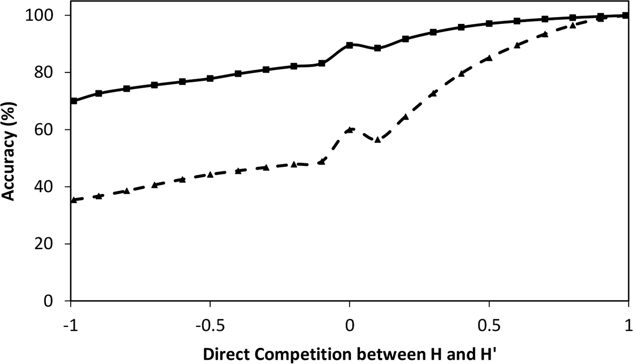
Results are presented in figure 4. Consider first of all the results for the general case (solid line). It is clear that as the degree of direct competition approaches its maximal value of 1, the accuracy of making inferences using the mutually exclusive model approaches 100%. This makes sense since maximal competition corresponds to mutual exclusion. While the accuracy of the mutually exclusive approach is greater than 97% for degrees of competition above about 0.5, in general the accuracy decreases as degree of direct competition decreases and is at 70% for values close to −1, which corresponds to the case in which the hypotheses, far from competing, entail each other. While this seems like a reasonable level of accuracy, it must be remembered that there are only two hypotheses to choose from, and so a random guess would achieve an accuracy of 50%. Note that a degree of competition of 0.5 corresponds to cases in which each hypothesis is on average still three times as likely to be true if the alternative hypothesis is false, $\mathrm{Pr}\left(H_i|\neg H_j\right)=3\times \mathrm{Pr}\left(H_i|H_j\right)$, while a degree of direct competition of 1/3 corresponds to the case in which each is on average still twice as likely. In such cases, there remains a substantial relation of negative relevance between the hypotheses, and thus reasoners may still be strongly inclined to think of them as competitors.Footnote ⁶

Figure 4.

Accuracy of inferences made using the mutually exclusive model as a function of the degree of direct competition between the hypotheses. Results are presented for the general case (solid line) and for the case in which all hypotheses with a posterior probability greater than 0.5 are taken into account in determining accuracy (dashed line).

Now consider the results that take into account cases in which both hypotheses H and H′ have a posterior probability greater than 0.5 according to the correct model (dashed line in fig. 4). When the degree of competition is 1, the hypotheses cannot both have probability greater than 0.5; that is, they cannot both be more likely to be true than false. Hence for high degrees of competition, the accuracy is still close to 100%. However, the accuracy now falls off much more quickly so that it is already below 75% when the degree of competition is 0.3. In general, the accuracy continues to fall with lower values of competition until it reaches an accuracy of just 35% as the degree of competition approaches −1. Of course, it is not surprising that the mutually exclusive approach performs worse in this case since according to it at most one hypothesis could be true (or have probability greater than 0.5). These results highlight the extent of perhaps the most significant problem with the mutually exclusive approach: its exclusion of hypotheses that may well be true.

In summary, insofar as inference is concerned with identifying the most probable hypothesis, it could be argued from the results in figure 4 that the mutually exclusive approach performs quite well, with an accuracy close to or greater than 90%, provided the hypotheses are in direct competition to at least some extent; that is, the degree of direct competition is greater than zero. However, the problem of excluding hypotheses that may well be true is a problem even in cases in which the hypotheses are competing. Of course, all of these results provide insight into cases in which we are only monitoring varying degrees of direct competition; future investigations will explore the extent to which these inaccuracies might be compounded when we instead consider cases of varying degrees of indirect or net competition.

5. Case Study

Let us return to our earlier discussion of consistent but competing scientific hypotheses in the context of the mass extinction at the K-Pg boundary. Here we focus on two of the causal hypotheses, asteroid impact and Deccan volcanism, which we denote as H and H′ respectively. There is no reason to think that these hypotheses are mutually exclusive. Yet, even if H and H′ do not compete at all along the direct pathway 2, they may still compete along the indirect pathway 1. If so, the discovery of evidence that provides confirmation of the impact hypothesis, as noted earlier, would count against volcanism via pathway 1 even if this evidence does not directly contradict volcanism. This is the main strategy adopted by Schulte et al. (Reference Schulte2010) who, assuming competition between the hypotheses, argue against volcanism essentially on the grounds that it is not needed because the asteroid hypothesis on its own accounts for the relevant evidence.

Some responses to Schulte et al. suggest that the impact and volcanism hypotheses are not in competition (Archibald et al. Reference Archibald2010; Courtillot and Fluteau Reference Courtillot and Fluteau2010; Keller et al. Reference Keller2010). Those arguments, as well as other work (Brusatte et al. Reference Brusatte2015), which relate to the first term in expression (2) and hence to pathway 1, amount to the claim that overall the evidence given both impact and volcanism hypotheses (and perhaps other hypotheses too) is much more probable than it is given the impact hypothesis without volcanism (i.e., $\mathrm{Pr}\left(E|H\&H^{\prime }\right)$ is much greater than $\mathrm{Pr}\left(E|H\&\neg H^{\prime }\right)$). In a recent paper, Renne et al. (Reference Renne2015) argue that the Chicxulub impact accelerated the rate of volcanic activity from the Deccan Traps. This kind of direct positive dependence between the hypotheses would result in a positive second term in (2) and would lead to support between the hypotheses rather than competition along pathway 2.

This very brief survey indicates that there are grounds for questioning the assumption that the impact and volcanic hypotheses are competing. Furthermore, even if the hypotheses are competing to some degree, the simulation results presented in section 4 show that if the assumption of mutual exclusion is made for inference purposes it could easily lead to exclusion of a true hypothesis.

6. Conclusion

We have argued that hypothesis competition cannot be adequately understood in terms of mutual exclusion. It is important to recognize that competition is a matter of degree and that it can occur in different ways—directly or indirectly via the evidence. In section 3, we defended a previously proposed measure by showing how it explicates these features in terms of degrees of direct and indirect competition and by illustrating its quantitative behavior in simple scenarios. It might be thought that mutual exclusivity would suffice as a simplifying assumption that would capture key aspects of scientific reasoning, but the results of computer simulations in section 4 show that this approach can have significant limitations, particularly by resulting in the exclusion of hypotheses that may well be true. Finally, our brief discussion of the extinction of the dinosaurs in section 5 illustrates subtleties of competition in scientific practice that go well beyond mutual exclusion. This work suggests that there is a need for philosophers of science to explore the nature of hypothesis competition in more detail, and we hope that our account provides a helpful framework for this task.