1 Introduction
In the last decade, growing computational power has led to an increasing number of numerical applications concerning three-dimensional problems in fluid dynamics. The validation of codes for these types of simulations is, however, difficult owing to the complexity of fully three-dimensional fluid motions. As a result, comparison with experiments would be desirable, even though these are not always available or may be difficult to handle because of a number of issues concerning the experimental measurements. In this context, the possibility of checking numerical codes against analytical solutions represents a considerable advantage since this allows for complete control of the physical quantities of interest and, from a numerical point of view, it makes the assignment of boundary/initial conditions very easy. Unfortunately, the availability of fully three-dimensional solutions for incompressible viscous fluids is very limited. With respect to this, a summary of analytic solutions can be found, for example, in Wang (Reference Wang1989) and Langlois & Deville (Reference Langlois and Deville2014).
The aim of the present work is, therefore, to make a further contribution in this direction. Specifically, we provide a class of unsteady tri-periodic fully three-dimensional solutions of the Navier–Stokes equations, basing on the work of Ethier-Ross & Steinman (Reference Ethier-Ross and Steinman1999). These correspond to laminar flows and can be gathered in two distinct solutions characterized by positive and negative helicity. In particular, they both belong to the class of Beltrami flows (where vorticity and velocity fields are parallel) and can be regarded as extensions in three dimensions of the well-known vortex solution by Taylor (Reference Taylor1923).
The benchmarking of numerical schemes is, obviously, the most straightforward application of the proposed analytical results. The periodicity of these solutions (and the consequent absence of boundaries) makes them particularly simple to use. In any case, this does not exhaust all possible applications of the proposed outcomes. Since such solutions represent the free evolution of rotational three-dimensional patterns, they can be adopted to study the onset of instabilities and the possible transition to turbulence in three-dimensional flows. This was, in fact, the original idea at the centre of the work by Taylor & Green (Reference Taylor and Green1937), where the initial evolution of a viscous fluid from a particular three-dimensional initial condition was studied. Such an initial condition was related to the bi-periodic vortex pattern described in Taylor (Reference Taylor1923) of which, in some sense, it represented an extension in three dimensions. At the present time, the above-mentioned approach is very common when dealing with numerical simulations of turbulence in three dimensions: the strategy is to initialize the computations through a three-dimensional divergence-free velocity field that extends the two-dimensional vortex pattern, and then study the subsequent evolution to turbulence (see Brachet et al. Reference Brachet, Meiron, Orszag, Nickel, Morf and Frisch1983; Berselli Reference Berselli2005; Drikakis et al. Reference Drikakis, Fureby, Grinstein and Youngs2007). Incidentally, we note that in many works the adopted three-dimensional initial condition is characterized by a null component in one direction (see, for example, Goldstein (Reference Goldstein1940), Orszag (Reference Orszag1974), Sharma & Sengupta (Reference Sharma and Sengupta2019)), and this implies longer times are needed to reach a fully developed homogeneous and isotropic turbulent flow. Such an issue may be easily overcome by using the proposed fully three-dimensional solutions. Similarly to the works of Di Mascio et al. (Reference Di Mascio, Antuono, Colagrossi and Marrone2017) and Sengupta, Sharma & Sengupta (Reference Sengupta, Sharma and Sengupta2018b) in which the stability of the two-dimensional solution by Taylor (Reference Taylor1923) was studied, the proposed solutions may represent a further tool for the inspection of the stability of three-dimensional flows and their transition to turbulence.
2 Solution structure
Here we briefly recall the solution structure described in Ethier-Ross & Steinman (Reference Ethier-Ross and Steinman1999). First, we introduce the Navier–Stokes equations for incompressible fluids, i.e.
 $$\begin{eqnarray}\displaystyle \left.\begin{array}{@{}c@{}}\displaystyle \unicode[STIX]{x1D735}\boldsymbol{\cdot }\boldsymbol{u}=0,\\ \displaystyle \frac{\unicode[STIX]{x2202}\boldsymbol{u}}{\unicode[STIX]{x2202}t}+(\boldsymbol{u}\boldsymbol{\cdot }\unicode[STIX]{x1D735})\boldsymbol{u}=-\frac{\unicode[STIX]{x1D735}p}{\unicode[STIX]{x1D70C}}+\unicode[STIX]{x1D708}\unicode[STIX]{x0394}\boldsymbol{u},\end{array}\right\} & & \displaystyle\end{eqnarray}$$
where  $\boldsymbol{u}=(u,v,w)$ is the velocity vector,
 $p$ is the pressure field,
 $\unicode[STIX]{x1D70C}$ is the density (constant) and
 $\unicode[STIX]{x1D708}$ is the kinematic viscosity. The class of solutions described in Ethier-Ross & Steinman (Reference Ethier-Ross and Steinman1999) are obtained by following an approach similar to that adopted for deriving the Taylor vortex solution (see Taylor (Reference Taylor1923)). Specifically, the strategy is to look for a divergence-free velocity field such that
(1) the unsteady terms (namely
 $\unicode[STIX]{x2202}\boldsymbol{u}/\unicode[STIX]{x2202}t$) balance the viscous terms in the momentum equations; and
(2) the advective terms
$(\boldsymbol{u}\boldsymbol{\cdot }\unicode[STIX]{x1D735})\boldsymbol{u}$ can be expressed as the gradient of a scalar function, that is, $(\boldsymbol{u}\boldsymbol{\cdot }\unicode[STIX]{x1D735})\boldsymbol{u}=\unicode[STIX]{x1D735}H,$ where $H$ is defined apart from an unessential constant value.


Since  $\boldsymbol{u}$ has to be divergence-free, the velocity field can be represented through the stream function
 $\unicode[STIX]{x1D74D}$ such that
 $\boldsymbol{u}=\unicode[STIX]{x1D735}\times \unicode[STIX]{x1D74D}$. Under the hypotheses above, the continuity equation is identically satisfied and the momentum equation can be rearranged as
 $$\begin{eqnarray}\displaystyle \unicode[STIX]{x1D735}\times \left[\frac{\unicode[STIX]{x2202}\unicode[STIX]{x1D74D}}{\unicode[STIX]{x2202}t}-\unicode[STIX]{x1D708}\unicode[STIX]{x0394}\unicode[STIX]{x1D74D}\right]=-\unicode[STIX]{x1D735}\left[\frac{p}{\unicode[STIX]{x1D70C}}+H\right]. & & \displaystyle\end{eqnarray}$$
The approach followed by Taylor (Reference Taylor1923) and later by Ethier-Ross & Steinman (Reference Ethier-Ross and Steinman1999) was to decompose the divergence-free field and the gradient field and obtain two separate equations, i.e.
 $$\begin{eqnarray}\displaystyle \frac{\unicode[STIX]{x2202}\unicode[STIX]{x1D74D}}{\unicode[STIX]{x2202}t}=\unicode[STIX]{x1D708}\unicode[STIX]{x0394}\unicode[STIX]{x1D74D},\quad \frac{p}{\unicode[STIX]{x1D70C}}+H=\text{const}. & & \displaystyle\end{eqnarray}$$
The idea above is of fundamental importance for the derivation of the analytical solutions, since it allows one to ‘move’ all the nonlinear contributions to the pressure field (through the term  $H$) and obtain a linear equation for the stream function
 $\unicode[STIX]{x1D74D}$. Incidentally, we observe that the second relation in (2.3) means that the mechanical energy, namely
 $E_{m}=p/\unicode[STIX]{x1D70C}+H$, remains constant during the flow evolution. For the first equation in (2.3), the following separation of variables is adopted:
 $$\begin{eqnarray}\displaystyle \unicode[STIX]{x1D74D}(\boldsymbol{x},t)=\unicode[STIX]{x1D733}(\boldsymbol{x})T(\unicode[STIX]{x1D70F}). & & \displaystyle\end{eqnarray}$$
Here  $\unicode[STIX]{x1D733}=(\unicode[STIX]{x1D6F9}_{yz},\unicode[STIX]{x1D6F9}_{zx},\unicode[STIX]{x1D6F9}_{xy})$ and
 $\unicode[STIX]{x1D70F}=\unicode[STIX]{x1D708}t$. Then, it follows that
 $$\begin{eqnarray}\displaystyle \frac{\text{d}T}{\text{d}\unicode[STIX]{x1D70F}}=\unicode[STIX]{x1D706}T,\quad \unicode[STIX]{x0394}\unicode[STIX]{x1D733}=\unicode[STIX]{x1D706}\unicode[STIX]{x1D733}, & & \displaystyle\end{eqnarray}$$
where  $\unicode[STIX]{x1D706}\in \mathbb{C}$. The first equation above gives
 $T(\unicode[STIX]{x1D70F})=\exp (\unicode[STIX]{x1D706}\unicode[STIX]{x1D70F})$, implying that
 $\text{Re}(\unicode[STIX]{x1D706})\leqslant 0$ is required in order to find bounded solutions for
 $\unicode[STIX]{x1D70F}>0$. To satisfy the second equation in (2.5), Ethier-Ross & Steinman (Reference Ethier-Ross and Steinman1999) adopted the following decomposition:
 $$\begin{eqnarray}\displaystyle \unicode[STIX]{x1D6F9}_{yz}=f(y)g(z)h(x),\quad \unicode[STIX]{x1D6F9}_{zx}=f(z)g(x)h(y),\quad \unicode[STIX]{x1D6F9}_{xy}=f(x)g(y)h(z). & & \displaystyle\end{eqnarray}$$
Here  $f,g$ and
 $h$ have to satisfy the relations
 $$\begin{eqnarray}\displaystyle \ddot{f}=a^{2}\,f,\quad \ddot{g}=b^{2}g,\quad \ddot{h}=c^{2}h, & & \displaystyle\end{eqnarray}$$
with  $\unicode[STIX]{x1D706}=a^{2}+b^{2}+c^{2}$ and
 $a,b,c\in \mathbb{C}$.
The last condition to fulfil is the requirement that  $(\boldsymbol{u}\boldsymbol{\cdot }\unicode[STIX]{x1D735})\boldsymbol{u}$ is a gradient. This is equivalent to imposing that
 $\unicode[STIX]{x1D735}\times [(\boldsymbol{u}\boldsymbol{\cdot }\unicode[STIX]{x1D735})\boldsymbol{u}]=0$. Using standard algebra, the latter condition corresponds to
 $$\begin{eqnarray}\displaystyle \unicode[STIX]{x1D735}\times [\boldsymbol{u}\times (\unicode[STIX]{x1D735}\times \boldsymbol{u})]=0. & & \displaystyle\end{eqnarray}$$
Flows satisfying the above equation are called generalized Beltrami flows. As a particular case, flows that satisfy (2.8) with  $\boldsymbol{u}\times (\unicode[STIX]{x1D735}\times \boldsymbol{u})=0$ are said to be Beltrami flows. The latter are characterized by a vorticity field which is always parallel to the velocity vector. Incidentally, we observe that Beltrami flows can never represent planar or axisymmetric motions, since in these latter cases the vorticity is always perpendicular to the velocity field. The role played by velocity, vorticity and their scalar product (namely helicity) is inspected, for example, Berselli & Cordoba (Reference Berselli and Cordoba2009) with a specific focus on the regularity of the flow evolution.
2.1 A brief review of the literature
Before describing the proposed solutions, we summarize here some of the available results obtained through the procedure described in the previous section.
As observed in Ethier-Ross & Steinman (Reference Ethier-Ross and Steinman1999), Taylor’s two-dimensional solution is obtained by setting  $\unicode[STIX]{x1D6F9}_{yz}=\unicode[STIX]{x1D6F9}_{xz}=0$ and
 $\unicode[STIX]{x1D6F9}_{xy}=f(x)g(y)$ (that is,
 $h=1$). This bi-periodic solution belongs to the generalized Beltrami flows and reads as
 $$\begin{eqnarray}\displaystyle \left.\begin{array}{@{}c@{}}u=-\cos (kx)\sin (ky)\text{e}^{-2\unicode[STIX]{x1D708}k^{2}t},\\ v=\sin (kx)\cos (ky)\text{e}^{-2\unicode[STIX]{x1D708}k^{2}t},\\ \displaystyle p=-\unicode[STIX]{x1D70C}\frac{\cos (2kx)+\cos (2ky)}{4}\text{e}^{-4\unicode[STIX]{x1D708}k^{2}t},\end{array}\right\} & & \displaystyle \nonumber\end{eqnarray}$$
where  $k=2\unicode[STIX]{x03C0}/L$ and
 $L$ is the wavelength. Sometimes this is erroneously referred to as the Taylor–Green vortex solution, but in the original work (i.e. Taylor Reference Taylor1923) Taylor is the unique author while both Taylor and Green appear in the subsequent paper (namely Taylor & Green Reference Taylor and Green1937) that is devoted to the analysis of the early stages of the evolution of a viscous fluid from periodic three-dimensional initial conditions.
In their work, Ethier-Ross & Steinman (Reference Ethier-Ross and Steinman1999) described a number of original solutions obtained through the procedure illustrated in § 2. In particular, they considered the following cases.
(i) Where
$a+b+c=0$ for $a,b,c\in \mathbb{R}$. This choice is, however, not useful for benchmarking because of the unbounded growth in time of the solution ($\text{Re}(\unicode[STIX]{x1D706})>0$).(ii) Where
$a^{2}+b^{2}=0$ and $c$ is purely imaginary. In this case, the solution belongs to a Beltrami flow and is made of exponentials and sine/cosine functions of the spatial variables that decay exponentially over time ($\text{Re}(\unicode[STIX]{x1D706})<0$).


In any case, not one of the motions above is tri-periodic and, consequently, an explicit modelling of the boundary of the computational domain is required for numerical simulations.
On the contrary, a tri-periodic solution obtained by using the approach of Ethier-Ross & Steinman (Reference Ethier-Ross and Steinman1999) is described in Barbato, Berselli & Grisanti (Reference Barbato, Berselli and Grisanti2007). Specifically, this is a Beltrami flow and corresponds to the choice  $a=c=0$ and
 $b=\imath k$ (namely
 $f=h=1$) and reads as
 $$\begin{eqnarray}\displaystyle \left.\begin{array}{@{}c@{}}u=[A\sin (kz)+C\cos (ky)]\text{e}^{-\unicode[STIX]{x1D708}k^{2}t},\\ v=[B\sin (kx)+A\cos (kz)]\text{e}^{-\unicode[STIX]{x1D708}k^{2}t},\\ w=[C\sin (ky)+B\cos (kx)]\text{e}^{-\unicode[STIX]{x1D708}k^{2}t},\\ \displaystyle p=-\unicode[STIX]{x1D70C}[BC\cos (kx)\sin (ky)+AB\sin (kx)\cos (kz)+AC\sin (kz)\cos (ky)]\text{e}^{-2\unicode[STIX]{x1D708}k^{2}t},\end{array}\right\}\quad & & \displaystyle\end{eqnarray}$$
where  $A,B$ and
 $C$ are arbitrary constants. Incidentally, we observe that this is not a fully three-dimensional motion, since the components of the velocity field do not depend on all the spatial variables (in particular,
 $u_{x}=v_{y}=w_{z}=0$).
Finally, we stress that the absence of boundaries in the domain makes periodic solutions particularly suited to study the onset of instabilities in the flow and the subsequent transition to turbulence numerically. Indeed, the fluid is free to evolve and is not influenced by the specific numerical treatment of the boundaries.
3 Tri-periodic fully three-dimensional solutions
Here we look for a tri-periodic fully three-dimensional solution of the form described in § 2. In particular, we simplify the problem by requiring the same periodicity in the three directions, namely  $a=b=c=\imath k,$ where
 $k$ is the wavenumber and
 $L=2\unicode[STIX]{x03C0}/k$ is the wavelength. Under these hypotheses, (2.7) gives
 $$\begin{eqnarray}\displaystyle & \displaystyle f(s)=A\cos (ks)+B\sin (ks), & \displaystyle\end{eqnarray}$$
 $$\begin{eqnarray}\displaystyle & \displaystyle g(s)=C\cos (ks)+D\sin (ks), & \displaystyle\end{eqnarray}$$
 $$\begin{eqnarray}\displaystyle & \displaystyle h(s)=E\cos (ks)+F\sin (ks). & \displaystyle\end{eqnarray}$$
The solution of (2.8) leads to a system of three nonlinear equations for the coefficients  $A,B,C,D,E$ and
 $F$ (see appendix A for details). After dropping the trivial cases (that is, those leading to a null velocity field), we find two distinct families of solutions:
 $$\begin{eqnarray}\displaystyle A_{1,2}=(r_{2,1})B,\quad C_{1,2}=(r_{1,2})D. & & \displaystyle\end{eqnarray}$$
Here the subscripts ‘1’ and ‘2’ indicate the specific family of the solution and
 $$\begin{eqnarray}\displaystyle r_{1}=\frac{\sqrt{3}E-F}{\sqrt{3}F+E},\quad r_{2}=\frac{\sqrt{3}E+F}{\sqrt{3}F-E}. & & \displaystyle\end{eqnarray}$$
We stress here that these may not be the unique non-trivial choices for the coefficients  $A,B,C,D,E$ and
 $F$ and that further solutions may exist. It is simple to prove that both families belong to the class of Beltrami flows and, in particular, the vorticity and velocity fields are linked by the relation
 $$\begin{eqnarray}\displaystyle \unicode[STIX]{x1D74E}_{1,2}=\pm \sqrt{3}k\boldsymbol{u}_{1,2}, & & \displaystyle\end{eqnarray}$$
which discriminates the two families according to the sign of the helicity field, namely  $\unicode[STIX]{x1D74E}\boldsymbol{\cdot }\boldsymbol{u}$. At present, we do not know whether the system reported in appendix A contains solutions of the general case
 $\unicode[STIX]{x1D735}\times [\boldsymbol{u}\times (\unicode[STIX]{x1D735}\times \boldsymbol{u})]=0$.
Before proceeding to the analysis, we note that, since the pressure gradient balances the nonlinear advective terms in the momentum equation and the vorticity is parallel to the velocity field, it immediately follows that
 $$\begin{eqnarray}\displaystyle \frac{\unicode[STIX]{x1D735}p}{\unicode[STIX]{x1D70C}}=-(\boldsymbol{u}\boldsymbol{\cdot }\unicode[STIX]{x1D735})\boldsymbol{u}=-\left[\unicode[STIX]{x1D735}\left(\frac{\Vert \boldsymbol{u}\Vert ^{2}}{2}\right)+\unicode[STIX]{x1D74E}\times \boldsymbol{u}\right]=-\unicode[STIX]{x1D735}\left(\frac{\Vert \boldsymbol{u}\Vert ^{2}}{2}\right), & & \displaystyle\end{eqnarray}$$
which implies that
 $$\begin{eqnarray}\displaystyle p_{1,2}=p_{0}-\unicode[STIX]{x1D70C}\frac{\Vert \boldsymbol{u}_{1,2}\Vert ^{2}}{2}, & & \displaystyle\end{eqnarray}$$
where  $p_{0}$ is a generic constant (hereinafter set equal to zero). Then, the knowledge of the velocity field immediately allows for the derivation of both the pressure and vorticity fields. Incidentally, we observe that the vortex stretching term is proportional to the gradient of the kinetic energy. Indeed, from (3.6), we find that
 $$\begin{eqnarray}\displaystyle {\mathcal{V}}_{1,2}^{S}=(\unicode[STIX]{x1D74E}_{1,2}\boldsymbol{\cdot }\unicode[STIX]{x1D735})\boldsymbol{u}_{1,2}=\pm \sqrt{3}k(\boldsymbol{u}_{1,2}\boldsymbol{\cdot }\unicode[STIX]{x1D735})\boldsymbol{u}_{1,2}=\pm \sqrt{3}k\unicode[STIX]{x1D735}\left(\frac{\Vert \boldsymbol{u}_{1,2}\Vert ^{2}}{2}\right), & & \displaystyle\end{eqnarray}$$
where the last equality is obtained following the derivation of (3.7). Then, the extrema of the kinetic energy field correspond to the points where the vortex stretching term is null.
3.1 One-parameter families
In this section we show that the two families of solutions described in (3.4) are actually characterized by just one parameter, namely  $R=F/E$. In particular, imposing the kinetic energy of the solution to be finite, it is possible to remove the apparent singularities at
 $R=\pm 1/\sqrt{3}$ in (3.5) to obtain
 $$\begin{eqnarray}\displaystyle u_{1,2} & = & \displaystyle \frac{4\sqrt{2}}{3\sqrt{3}} [\!\sin (kx+\unicode[STIX]{x1D703}_{1,2})\cos (ky+\unicode[STIX]{x1D719}_{1,2})\sin (kz+\unicode[STIX]{x1D713}_{1,2})\nonumber\\ \displaystyle & & \displaystyle -\cos (kz+\unicode[STIX]{x1D703}_{1,2})\sin (kx+\unicode[STIX]{x1D719}_{1,2})\sin (ky+\unicode[STIX]{x1D713}_{1,2})\!]\text{e}^{-3\unicode[STIX]{x1D708}k^{2}t}U_{0},\end{eqnarray}$$
 $$\begin{eqnarray}\displaystyle v_{1,2} & = & \displaystyle \frac{4\sqrt{2}}{3\sqrt{3}} [\!\sin (ky+\unicode[STIX]{x1D703}_{1,2})\cos (kz+\unicode[STIX]{x1D719}_{1,2})\sin (kx+\unicode[STIX]{x1D713}_{1,2})\nonumber\\ \displaystyle & & \displaystyle -\cos (kx+\unicode[STIX]{x1D703}_{1,2})\sin (ky+\unicode[STIX]{x1D719}_{1,2})\sin (kz+\unicode[STIX]{x1D713}_{1,2})\!]\text{e}^{-3\unicode[STIX]{x1D708}k^{2}t}U_{0},\end{eqnarray}$$
 $$\begin{eqnarray}\displaystyle w_{1,2} & = & \displaystyle \frac{4\sqrt{2}}{3\sqrt{3}} [\!\sin (kz+\unicode[STIX]{x1D703}_{1,2})\cos (kx+\unicode[STIX]{x1D719}_{1,2})\sin (ky+\unicode[STIX]{x1D713}_{1,2})\nonumber\\ \displaystyle & & \displaystyle -\cos (ky+\unicode[STIX]{x1D703}_{1,2})\sin (kz+\unicode[STIX]{x1D719}_{1,2})\sin (kx+\unicode[STIX]{x1D713}_{1,2})\!]\text{e}^{-3\unicode[STIX]{x1D708}k^{2}t}U_{0},\end{eqnarray}$$
where  $U_{0}$ is the reference velocity. By construction (see appendix A), the latter is related to the averaged kinetic energy per unit of mass, i.e
 $$\begin{eqnarray}\displaystyle \overline{{\mathcal{E}}}(t)=\frac{1}{L^{3}}\int _{0}^{L}\int _{0}^{L}\int _{0}^{L}\frac{\Vert \boldsymbol{u}\Vert ^{2}}{2}\,\text{d}x\,\text{d}y\,\text{d}z=\frac{U_{0}^{2}}{2}\text{e}^{-6\unicode[STIX]{x1D708}k^{2}t}, & & \displaystyle\end{eqnarray}$$
so that  $\overline{{\mathcal{E}}}(0)=U_{0}^{2}/2$ at the initial time. The phases
 $\unicode[STIX]{x1D703}_{1},\unicode[STIX]{x1D719}_{1}$ and
 $\unicode[STIX]{x1D713}_{1}$ are given by the following relations:
 $$\begin{eqnarray}\displaystyle & \displaystyle (\sin \unicode[STIX]{x1D703}_{1},\cos \unicode[STIX]{x1D703}_{1})=\left(-\frac{\sqrt{3}+R}{2\sqrt{1+R^{2}}},\frac{1-\sqrt{3}R}{2\sqrt{1+R^{2}}}\right), & \displaystyle\end{eqnarray}$$
 $$\begin{eqnarray}\displaystyle & \displaystyle (\sin \unicode[STIX]{x1D719}_{1},\cos \unicode[STIX]{x1D719}_{1})=\left(\frac{\sqrt{3}-R}{2\sqrt{1+R^{2}}},\frac{1+\sqrt{3}R}{2\sqrt{1+R^{2}}}\right), & \displaystyle\end{eqnarray}$$
 $$\begin{eqnarray}\displaystyle & \displaystyle (\sin \unicode[STIX]{x1D713}_{1},\cos \unicode[STIX]{x1D713}_{1})=\left(\frac{1}{\sqrt{1+R^{2}}},\frac{R}{\sqrt{1+R^{2}}}\right). & \displaystyle\end{eqnarray}$$
Using standard trigonometric identities, we obtain
 $$\begin{eqnarray}\displaystyle & \displaystyle (\sin (\unicode[STIX]{x1D703}_{1}-\unicode[STIX]{x1D713}_{1}),\cos (\unicode[STIX]{x1D703}_{1}-\unicode[STIX]{x1D713}_{1}))=\left(-{\textstyle \frac{1}{2}},-{\textstyle \frac{\sqrt{3}}{2}}\right), & \displaystyle \nonumber\\ \displaystyle & \displaystyle (\sin (\unicode[STIX]{x1D719}_{1}-\unicode[STIX]{x1D713}_{1}),\cos (\unicode[STIX]{x1D719}_{1}-\unicode[STIX]{x1D713}_{1}))=\left(-{\textstyle \frac{1}{2}},+{\textstyle \frac{\sqrt{3}}{2}}\right), & \displaystyle \nonumber\end{eqnarray}$$
which lead to
 $$\begin{eqnarray}\displaystyle \unicode[STIX]{x1D703}_{1}=\unicode[STIX]{x1D713}_{1}-\frac{5}{6}\unicode[STIX]{x03C0},\quad \unicode[STIX]{x1D719}_{1}=\unicode[STIX]{x1D713}_{1}-\frac{\unicode[STIX]{x03C0}}{6},\quad \text{where}~\unicode[STIX]{x1D713}_{1}=\arccos \left(\frac{R}{\sqrt{1+R^{2}}}\right).\qquad & & \displaystyle\end{eqnarray}$$
For the second family of solutions, we find that  $\unicode[STIX]{x1D703}_{2}=\unicode[STIX]{x1D719}_{1}$,
 $\unicode[STIX]{x1D719}_{2}=\unicode[STIX]{x1D703}_{1}$ and
 $\unicode[STIX]{x1D713}_{2}=\unicode[STIX]{x1D713}_{1}=\unicode[STIX]{x1D713},$ where the symbol
 $\unicode[STIX]{x1D713}$ is used hereinafter for the sake of notation.
A detailed inspection of the above findings shows that the parameter  $R$ (or, equivalently, the angle
 $\unicode[STIX]{x1D713}$) corresponds to a translation of the solutions of both families in the direction
 $(1,1,1)$. From a different perspective, we can represent each family through a reference solution and translate it in the direction
 $(1,1,1)$ through different choices of
 $R$ (or
 $\unicode[STIX]{x1D713}$). In particular, through the translation
 $$\begin{eqnarray}\displaystyle (x^{\prime },y^{\prime },z^{\prime })=(x,y,z)+\frac{\unicode[STIX]{x1D713}}{k}(1,1,1), & & \displaystyle\end{eqnarray}$$
we can rearrange (3.10)–(3.12) for family ‘1’ into the following reference solution:
 $$\begin{eqnarray}\displaystyle \begin{array}{@{}rcl@{}}\displaystyle \frac{u_{1}}{U_{0}}\ & =\ & {\displaystyle \frac{4\sqrt{2}}{3\sqrt{3}}}\left[\sin \left(kx^{\prime }-{\displaystyle \frac{5}{6}}\unicode[STIX]{x03C0}\right)\cos \left(ky^{\prime }-{\displaystyle \frac{\unicode[STIX]{x03C0}}{6}}\right)\sin (kz^{\prime })\right.\\ \ & \ & -\left.\cos \left(kz^{\prime }-{\displaystyle \frac{5}{6}}\unicode[STIX]{x03C0}\right)\sin \left(kx^{\prime }-{\displaystyle \frac{\unicode[STIX]{x03C0}}{6}}\right)\sin (ky^{\prime })\right]\text{e}^{-3\unicode[STIX]{x1D708}k^{2}t},\\ \displaystyle \frac{v_{1}}{U_{0}}\ & =\ & {\displaystyle \frac{4\sqrt{2}}{3\sqrt{3}}}\left[\sin \left(ky^{\prime }-{\displaystyle \frac{5}{6}}\unicode[STIX]{x03C0}\right)\cos \left(kz^{\prime }-{\displaystyle \frac{\unicode[STIX]{x03C0}}{6}}\right)\sin (kx^{\prime })\right.\\ \ & \ & -\left.\cos \left(kx^{\prime }-{\displaystyle \frac{5}{6}}\unicode[STIX]{x03C0}\right)\sin \left(ky^{\prime }-{\displaystyle \frac{\unicode[STIX]{x03C0}}{6}}\right)\sin (kz^{\prime })\right]\text{e}^{-3\unicode[STIX]{x1D708}k^{2}t},\\ \displaystyle \frac{w_{1}}{U_{0}}\ & =\ & {\displaystyle \frac{4\sqrt{2}}{3\sqrt{3}}}\left[\sin \left(kz^{\prime }-{\displaystyle \frac{5}{6}}\unicode[STIX]{x03C0}\right)\cos \left(kx^{\prime }-{\displaystyle \frac{\unicode[STIX]{x03C0}}{6}}\right)\sin (ky^{\prime })\right.\\ \ & \ & -\left.\cos \left(ky^{\prime }-{\displaystyle \frac{5}{6}}\unicode[STIX]{x03C0}\right)\sin \left(kz^{\prime }-{\displaystyle \frac{\unicode[STIX]{x03C0}}{6}}\right)\sin (kx^{\prime })\right]\text{e}^{-3\unicode[STIX]{x1D708}k^{2}t}.\end{array} & & \displaystyle \nonumber\end{eqnarray}$$
Here the dependence on the parameter  $R$ is dropped. The reference solution for family ‘2’ is obtained by interchanging the angles
 $5\unicode[STIX]{x03C0}/6$ and
 $\unicode[STIX]{x03C0}/6$.
Going back to the original variables, the stagnation points of the above solutions can be calculated by solving the latter system:
 $$\begin{eqnarray}\displaystyle \sin (kx+\unicode[STIX]{x1D713})=0,\quad \sin (ky+\unicode[STIX]{x1D713})=0,\quad \sin (kz+\unicode[STIX]{x1D713})=0. & & \displaystyle\end{eqnarray}$$
Note that both families share the same positions of the stagnation points and these are placed over the regular lattice
 $$\begin{eqnarray}(x_{l},y_{m},z_{n})=-\frac{\unicode[STIX]{x1D713}}{k}(1,1,1)-\frac{\unicode[STIX]{x03C0}}{k}(l,m,n),\end{eqnarray}$$
where  $l,m,n\in \mathbb{Z}$. In § A.1 we provide a linear stability analysis of the stagnation points and prove that they are always unstable equilibria. The above findings do not depend on the parameter
 $R$ (since this just represents a translation) and the only difference between the two families is the reversal of the stable/unstable manifolds. The same behaviour occurs between the different stagnation points belonging to the same family. As pointed out in Sharma & Sengupta (Reference Sharma and Sengupta2019), the presence of unstable equilibria may be the triggering for a period-doubling bifurcation and, subsequently, for a possible transition to the turbulent regime.
3.2 Examples
Here we show some plots of the proposed solutions. In particular, we display them at the initial time, namely  $t=0$, since the later instants just represent a damping of the initial velocity distribution. We consider dimensionless variables
 $\boldsymbol{x}^{\ast }=\boldsymbol{x}/L$,
 $\boldsymbol{u}^{\ast }=\boldsymbol{u}/U_{0}$ and
 $p^{\ast }=p/(\unicode[STIX]{x1D70C}U_{0}^{2})$ and, without any loss of generality, choose
 $R=0$ for both families. This latter choice is motivated by the necessity of simplifying the graphical representation of the stagnation points in the reference domain, namely the three-dimensional torus
 $[0,1]^{3}$.
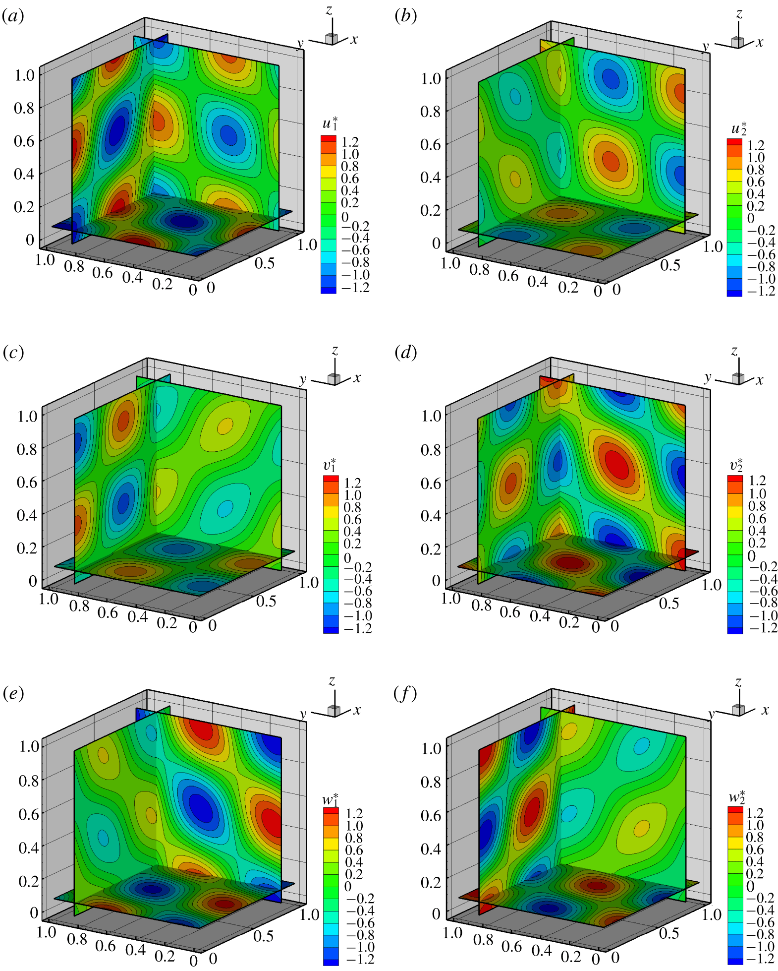
Contours of the velocity fields  $\boldsymbol{u}_{1}^{\ast }$ (a,c,e) and
 $\boldsymbol{u}_{2}^{\ast }$ (b,d,f) for
 $R=0$ (slices at
 $x^{\ast }=0.86$,
 $y^{\ast }=0.86$ and
 $z^{\ast }=0.08$).

In figure 1 we show the contours of the fields  $\boldsymbol{u}_{1}^{\ast }=(u_{1}^{\ast },v_{1}^{\ast },w_{1}^{\ast })$ (a,c,e) and
 $\boldsymbol{u}_{2}^{\ast }=(u_{2}^{\ast },v_{2}^{\ast },w_{2}^{\ast })$ (b,d,f) along the planes
 $x^{\ast }=0.86$,
 $y^{\ast }=0.86$ and
 $z^{\ast }=0.08$. The two families display similar patterns for the velocity components even though these show different orientations/angles of the contour lines. We note that some of these patterns are very close to the two-dimensional Taylor–Green vortex solution (see, for example, the planes at
 $y^{\ast }=0.86$ and
 $z^{\ast }=0.08$ of the component
 $v_{1}^{\ast }$ in figure 1c).
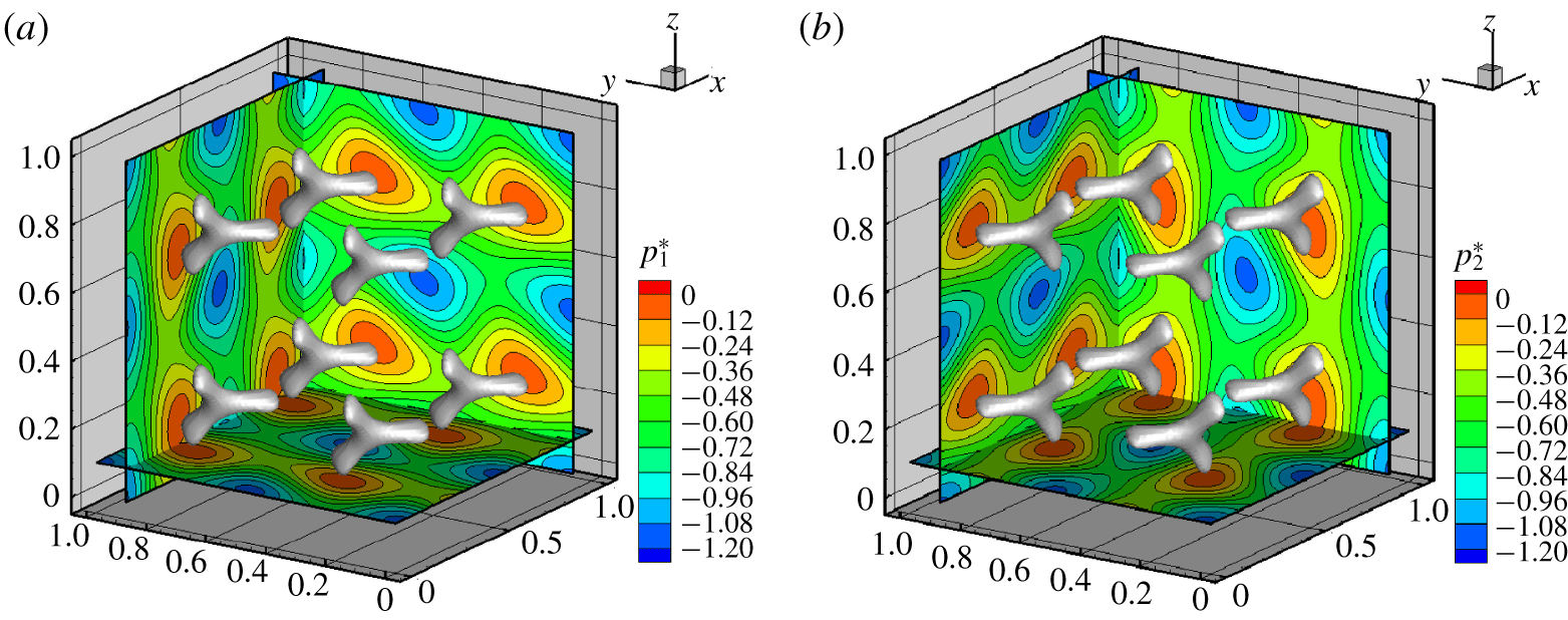
Contours of the pressure fields  $p_{1}^{\ast }$ (a) and
 $p_{2}^{\ast }$ (b) for
 $R=0$ (slices at
 $x^{\ast }=0.86$,
 $y^{\ast }=0.86$ and
 $z^{\ast }=0.08$) and iso-surfaces at
 $p_{1}^{\ast }=-0.02$ (a) and
 $p_{2}^{\ast }=-0.02$ (b).

In figure 2 we show the contours of the pressure fields  $p_{1}^{\ast }$ and
 $p_{2}^{\ast }$ on the same planes. Since the pressure directly relates to the kinetic energy and to the enstrophy (i.e.
 $\Vert \unicode[STIX]{x1D74E}\Vert ^{2}/2$), we also plot the iso-surfaces for
 $p_{1}^{\ast }=p_{2}^{\ast }=-0.02$. These highlight the presence of a pattern of
 $Y$-shaped structures that identify the regions where the enstrophy and the kinetic energy of the solutions are smaller, that is, the regions containing the stagnation points. For
 $R=0,$ these are obtained by solving the system (3.19) and read as
 $$\begin{eqnarray}\displaystyle (x_{l}^{\ast },y_{m}^{\ast },z_{n}^{\ast })=-{\textstyle \frac{1}{4}}(1,1,1)+{\textstyle \frac{1}{2}}(l,m,n), & & \displaystyle\end{eqnarray}$$
where  $l,m,n\in \mathbb{Z}$. It is interesting to observe that the
 $Y$-shaped structures have different orientations between the two families but ‘lie’ on the same planes, that is, planes orthogonal to the direction
 $(1,1,1)$. The latter is the direction associated with the maximum absolute eigenvalue at the stagnation points, as described in § A.1.
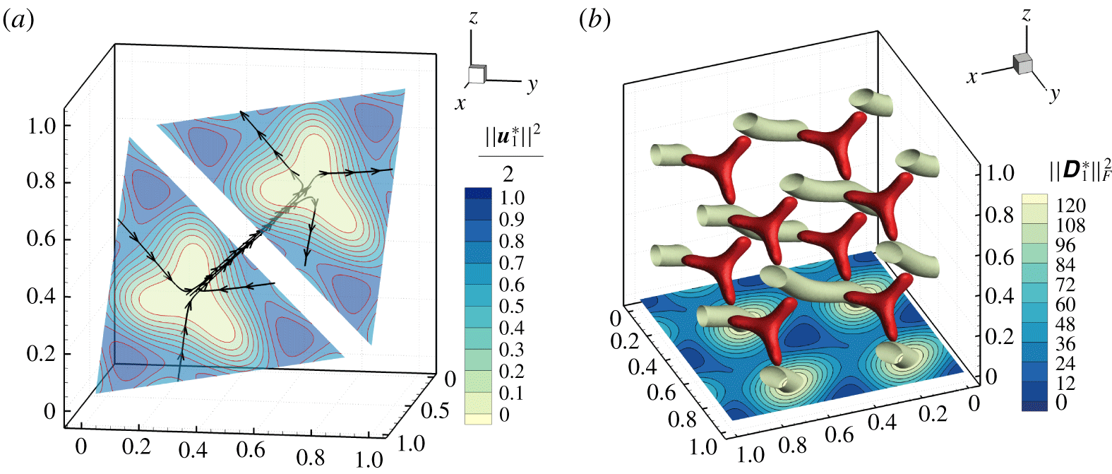
For family ‘1’, we show in figure 3(a) the streamlines in the neighbourhood of the stagnation points  $(1/4,1/4,1/4)$ and
 $(3/4,3/4,3/4)$ along with the planes that pass through them and are orthogonal to the direction
 $(1,1,1)$. Along these planes the contours of the kinetic energy
 $\Vert \boldsymbol{u}_{1}^{2}\Vert /2$ are drawn, highlighting the projection of the
 $Y$-shaped structures in the neighbourhood of the stagnation points. In figure 3(b) we show the
 $Y$-shaped structures along with the iso-surfaces and contours of
 $\Vert \unicode[STIX]{x1D63F}_{1}^{\ast }\Vert _{F}^{2}=\unicode[STIX]{x1D63F}_{1}^{\ast }\boldsymbol{ : }\unicode[STIX]{x1D63F}_{1}^{\ast },$ where
 $\unicode[STIX]{x1D63F}_{1}^{\ast }$ is the strain-rate tensor (namely the symmetric part of the tensor
 $\unicode[STIX]{x1D735}^{\ast }\boldsymbol{u}_{1}^{\ast }$) and
 $\Vert \cdot \Vert _{F}$ denotes the Frobenius matrix norm. The regions where the norm of the strain-rate tensor is close to the maximum value (about 120) appear like tubular shapes and are approximately oriented along the vector
 $(1,1,1)$, though they are separate from the neighbourhoods of the stagnation points. Note that the maximum of
 $\Vert \unicode[STIX]{x1D63F}_{1}^{\ast }\Vert _{F}^{2}$ is much larger than the enstrophy field (whose maximum is about
 $0.1$). The same behaviour is observed for family ‘2’ and is therefore not displayed here.
(a) Streamlines close to the stagnation points  $(1/4,1/4,1/4)$ and
 $(3/4,3/4,3/4)$. Here the planes are orthogonal to the direction
 $(1,1,1)$ and display the contour of the kinetic energy
 $\Vert \boldsymbol{u}_{1}^{\ast }\Vert ^{2}/2$. (b) Contour of
 $\Vert \unicode[STIX]{x1D63F}_{1}^{\ast }\Vert _{F}^{2}$ on the plane
 $z^{\ast }=0$ and iso-surface at
 $\Vert \unicode[STIX]{x1D63F}_{1}^{\ast }\Vert _{F}^{2}=115$ (here the ‘
 $Y$’-shaped structures correspond to the iso-surface of the enstrophy at
 $\Vert \unicode[STIX]{x1D74E}_{1}^{\ast }\Vert ^{2}/2=0.0015$). In both the panels
 $R=0$.

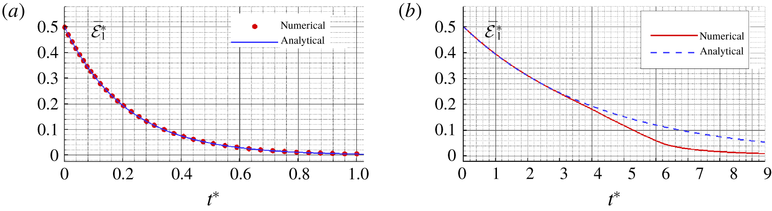
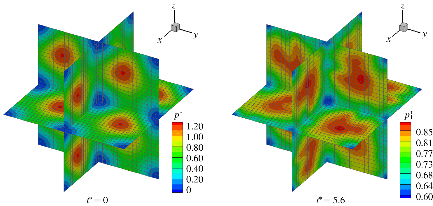
As a proof of concept of the possible applications related to the proposed solutions, we present in figure 4 the time histories of the averaged kinetic energy per unit of mass (see (3.13)) as predicted by the theoretical solution and by a finite volume code (see Di Mascio, Muscari & Dubbioso Reference Di Mascio, Muscari and Dubbioso2014; Muscari, Dubbioso & Di Mascio Reference Muscari, Dubbioso and Di Mascio2017). In particular, we define the Reynolds number as  $Re=U_{0}L/\unicode[STIX]{x1D708}$ and consider the cases
 $Re=50$ (figure 4a) and
 $Re=1000$ (figure 4b). In both simulations a uniform grid of
 $32^{3}$ points has been used. In the former case, the numerical output is practically superimposed to the analytical solution during the entire interval of the simulation which confirms the accuracy of the numerical algorithm. On the contrary, for
 $Re=1000$ some instabilities arise at about
 $t^{\ast }=3$, leading to an increase of dissipation and a deviation from the theoretical solution. For this latter case, we show in figure 5 the evolution of the pressure field along the three-coordinate planes at the centre of the domain. In particular, the left plot shows the initial pressure field (given by the analytic solution) while the right plot displays the solution at
 $t^{\ast }=5.6$. At this time instant the breaking down of the analytical vortex pattern and the generation of smaller wavelengths is evident.
Time histories of the averaged kinetic energy per unit of mass for  $Re=50$ (a) and
 $Re=1000$ (b). Comparisons between the analytic solutions and the numerical outputs. In both panels the solution for family ‘1’ when
 $R=0$ has been used to initialize the computations.

Snapshots of the evolution of the pressure field at  $Re=1000$ as predicted by the numerical solver. The analytical solution for family ‘1’ when
 $R=0$ has been used to initialize the computations.

The above findings suggest that the proposed solutions may be suited to study the triggering of instabilities and the transition to turbulence in high-Reynolds-number flows. Furthermore, they may be used for a receptivity/instability analysis based on disturbance enstrophy as described, for example, in Sengupta et al. (Reference Sengupta, Suman, Sengupta and Bhaumik2018a). In any case, these topics are beyond the scope of the present work.
4 Some considerations about turbulence
In both the introduction and the previous section we stressed that the proposed solutions may be used to study the onset of instabilities in the laminar flow and the subsequent possible transition to the turbulent regime. This likely occurs for high-Reynolds-number flows. Conversely, when the Reynolds number is very low, the proposed solutions may also be employed to characterize turbulent flows close to the Kolmogorov microscale.
In particular, using (3.13), we define the reference rate of energy dissipation as
 $$\begin{eqnarray}\displaystyle \unicode[STIX]{x1D716}=\left.\frac{\text{d}\overline{{\mathcal{E}}}(t)}{\text{d}t}\right|_{t=0}=\unicode[STIX]{x1D708}k^{2}U_{0}^{2}, & & \displaystyle\end{eqnarray}$$
where the equality is hereinafter understood as a relation between orders of magnitude (i.e. all numerical values are dropped). Then, defining the Reynolds number as  $Re=U_{0}L/\unicode[STIX]{x1D708}$, we consider the case
 $Re=1$. As a consequence,
 $U_{0}=\unicode[STIX]{x1D708}/L$ which leads to
 $$\begin{eqnarray}\displaystyle \unicode[STIX]{x1D716}=k^{2}\frac{\unicode[STIX]{x1D708}^{3}}{L^{2}}=\frac{\unicode[STIX]{x1D708}^{3}}{L^{4}},\quad \Rightarrow \quad L=\left(\frac{\unicode[STIX]{x1D708}^{3}}{\unicode[STIX]{x1D716}}\right)^{1/4}, & & \displaystyle\end{eqnarray}$$
which is exactly the Kolmogorov length scale. The time scale is immediately obtained by setting  $T=L/U_{0}=L^{2}/\unicode[STIX]{x1D708}$.
The reason why we rediscover the Kolmogorov microscale relies in the decomposition described in § 2. This implies that all the energy related to the generation of nonlinearities (i.e. the term  $(\boldsymbol{u}\boldsymbol{\cdot }\unicode[STIX]{x1D735})\,\boldsymbol{u}$) is ‘absorbed’ by the pressure field and gives no contribution to the time derivative
 $\unicode[STIX]{x2202}\boldsymbol{u}/\unicode[STIX]{x2202}t$. Consequently, no smaller length scales are created and, thus, the dynamics is dominated by viscous dissipation. This probably means that the flow at the Kolmogorov microscale tends to be a Beltrami flow (generalized or not).
5 Conclusions
Tri-periodic fully three-dimensional analytic solutions of the Navier–Stokes equations have been derived basing on the work of Ethier-Ross & Steinman (Reference Ethier-Ross and Steinman1999). These belong to the class of Beltrami flows and can be gathered in two distinct solutions characterized by positive and negative helicity. In particular, some plots of the proposed solutions have been displayed, showing that these can be regarded as a generalization in three dimensions of the Taylor–Green vortex solution. Furthermore, numerical simulations have been considered in order to illustrate the possible applications related to the theoretical findings.
The proposed solutions are simple to implement and to use for benchmarking numerical codes because, owing to their periodicity, there is no need for an explicit modelling of boundaries. Finally, they may be adopted to study the onset of turbulence in high-Reynolds-number flows, since they represent the free evolution of rotational three-dimensional fluid patterns.
Acknowledgements
This research was developed within and supported by the MIUR PRIN 2017 Project ‘FUNdamentals of BREAKing wave-induced boundary dynamics – FUNBREAK’, grant number 20172B7MY9. Useful discussions with Dr A. Colagrossi, Dr S. Marrone and Professor A. Di Mascio are gratefully acknowledged. In particular, the author thanks Dr S. Marrone and Professor A. Di Mascio for the numerical simulations shown in the present paper.
Declaration of interests
The authors report no conflict of interest.
Appendix A. Details of the computation
The substitution of the functions (3.1)–(3.3) in (2.7) and, subsequently, in (2.8) leads to a complex expression made of sines/cosines of the spatial coordinates. This can be regarded as a Fourier series in the variables  $(x,y,z)$ containing a finite number of modes whose amplitudes are made of the coefficients
 $A,B,C,D,E$ and
 $F$ of (3.1)–(3.3). Since the number of terms in the above expression is large, the amplitudes of the different modes are obtained by using the standard integral relations of a Fourier series through the Maple software for symbolic and numeric computing. Dropping multiple or linear dependent outputs, we find the following nonlinear system:
 $$\begin{eqnarray}\displaystyle \left.\begin{array}{@{}l@{}}B^{2}C^{2}FE+A^{2}D^{2}FE-B^{2}CF^{2}D-AD^{2}F^{2}B\\ \quad -\,A^{2}CE^{2}D-AC^{2}E^{2}B-6BCFADE=0,\\ -A^{2}C^{2}E^{2}-BCE^{2}AD+ADF^{2}BC-B^{2}C^{2}F^{2}+A^{2}D^{2}E^{2}-A^{2}D^{2}F^{2}\\ \quad +\,B^{2}C^{2}E^{2}+BD^{2}FAE+B^{2}DFCE-BC^{2}FAE-A^{2}DFCE+B^{2}D^{2}F^{2}=0,\\ A^{2}D^{2}F^{2}+2A^{2}DFCE-2BC^{2}FAE-B^{2}C^{2}F^{2}\\ \quad -\,2BD^{2}FAE+B^{2}C^{2}E^{2}+2B^{2}DFCE-A^{2}D^{2}E^{2}=0.\end{array}\right\} & & \displaystyle \nonumber\end{eqnarray}$$
Using the Maple software, we find some trivial solutions (which are dropped) and the two families of solutions described in (3.4). Substituting these in the expressions (3.1)–(3.3) and introducing the new parameter  $R=F/E$, we find that
 $$\begin{eqnarray}\displaystyle u & = & \displaystyle kBDE\left\{\left[\left(\frac{A_{1,2}}{B}\right)\cos (kx)+\sin (kx)\right]\left[-\left(\frac{C_{1,2}}{D}\right)\sin (ky)+\cos (ky)\right]\right.\nonumber\\ \displaystyle & & \displaystyle \times \,[\cos (kz)+R\sin (kz)]-\left[-\left(\frac{A_{1,2}}{B}\right)\sin (kz)+\cos (kz)\right]\nonumber\\ \displaystyle & & \displaystyle \times \left.\!\left[\left(\frac{C_{1,2}}{D}\right)\cos (kx)+\sin (kx)\right][\cos (ky)+R\sin (ky)]\right\}\text{e}^{-3\unicode[STIX]{x1D708}k^{2}t},\nonumber\end{eqnarray}$$
 $$\begin{eqnarray}\displaystyle v & = & \displaystyle kBDE\left\{\left[\left(\frac{A_{1,2}}{B}\right)\cos (ky)+\sin (ky)\right]\left[-\left(\frac{C_{1,2}}{D}\right)\sin (kz)+\cos (kz)\right]\right.\nonumber\\ \displaystyle & & \displaystyle \times \,[\cos (kx)+R\sin (kx)]-\left[-\left(\frac{A_{1,2}}{B}\right)\sin (kx)+\cos (kx)\right]\nonumber\\ \displaystyle & & \displaystyle \times \left.\!\left[\left(\frac{C_{1,2}}{D}\right)\cos (ky)+\sin (ky)\right][\cos (kz)+R\sin (kz)]\right\}\text{e}^{-3\unicode[STIX]{x1D708}k^{2}t},\nonumber\end{eqnarray}$$
 $$\begin{eqnarray}\displaystyle w & = & \displaystyle kBDE\left\{\left[\left(\frac{A_{1,2}}{B}\right)\cos (kz)+\sin (kz)\right]\left[-\left(\frac{C_{1,2}}{D}\right)\sin (kx)+\cos (kx)\right]\right.\nonumber\\ \displaystyle & & \displaystyle \times \,[\cos (ky)+R\sin (ky)]-\left[-\left(\frac{A_{1,2}}{B}\right)\sin (ky)+\cos (ky)\right]\nonumber\\ \displaystyle & & \displaystyle \times \left.\!\left[\left(\frac{C_{1,2}}{D}\right)\cos (kz)+\sin (kz)\right][\cos (kx)+R\sin (kx)]\right\}\text{e}^{-3\unicode[STIX]{x1D708}k^{2}t},\nonumber\end{eqnarray}$$
where the subscripts ‘1’ and ‘2’ indicate the specific family of the solution and
 $$\begin{eqnarray}\displaystyle A_{1,2}=(r_{2,1})B,\quad C_{1,2}=(r_{1,2})D, & & \displaystyle\end{eqnarray}$$
where
 $$\begin{eqnarray}\displaystyle r_{1}=\frac{\sqrt{3}-R}{\sqrt{3}R+1},\quad r_{2}=\frac{\sqrt{3}+R}{\sqrt{3}R-1}. & & \displaystyle\end{eqnarray}$$
First, we observe that the coefficients  $B$,
 $D$ and
 $E$ are redundant and can be replaced by a single parameter
 $H=kBDE$. Furthermore, we note that the solution is formally singular for
 $R=\pm 1/\sqrt{3}$. It is simple to show that such singularities are apparent and can be eliminated by imposing a finite value of the averaged kinetic energy per unity of mass. In particular, we obtain
 $$\begin{eqnarray}\displaystyle \overline{{\mathcal{E}}}(t)=\frac{1}{L^{3}}\int _{0}^{L}\int _{0}^{L}\int _{0}^{L}\frac{\Vert \boldsymbol{u}\Vert ^{2}}{2}\,\text{d}x\,\text{d}y\,\text{d}z=\frac{27}{4}\frac{(1+R^{2})^{3}}{(1-3R^{2})^{2}}\text{e}^{-6\unicode[STIX]{x1D708}k^{2}t}H^{2}. & & \displaystyle\end{eqnarray}$$
We require  $\overline{{\mathcal{E}}}(t)$ at
 $t=0$ to be finite and define the reference velocity
 $U_{0}$ such that
 $\overline{{\mathcal{E}}}(0)=U_{0}^{2}/2$. As a consequence, we obtain the following expression for
 $H$:
 $$\begin{eqnarray}\displaystyle H=\frac{\sqrt{2}}{3\sqrt{3}}\frac{(1-3R^{2})}{(1+R^{2})^{3/2}}U_{0}. & & \displaystyle\end{eqnarray}$$
Substituting the above formula in the equations for  $\boldsymbol{u}=(u,v,w)$ and rearranging, we obtain
 $$\begin{eqnarray}\displaystyle u_{1,2} & = & \displaystyle {\textstyle \frac{4\sqrt{2}}{3\sqrt{3}}}\left\{[a_{1,2}\cos (kx)+b_{1,2}\sin (kx)][-c_{1,2}\sin (ky)+d_{1,2}\cos (ky)]\right.\nonumber\\ \displaystyle & & \displaystyle \times \,[e_{1,2}\cos (kz)+f_{1,2}\sin (kz)]-[-a_{1,2}\sin (kz)+b_{1,2}\cos (kz)]\nonumber\\ \displaystyle & & \displaystyle \times \left.[c_{1,2}\cos (kx)+d_{1,2}\sin (kx)][e_{1,2}\cos (ky)+f_{1,2}\sin (ky)]\right\}\text{e}^{-3\unicode[STIX]{x1D708}k^{2}t}U_{0},\nonumber\end{eqnarray}$$
 $$\begin{eqnarray}\displaystyle v_{1,2} & = & \displaystyle {\textstyle \frac{4\sqrt{2}}{3\sqrt{3}}}\left\{[a_{1,2}\cos (ky)+b_{1,2}\sin (ky)][-c_{1,2}\sin (kz)+d_{1,2}\cos (kz)]\right.\nonumber\\ \displaystyle & & \displaystyle \times \,[e_{1,2}\cos (kx)+f_{1,2}\sin (kx)]-[-a_{1,2}\sin (kx)+b_{1,2}\cos (kx)]\nonumber\\ \displaystyle & & \displaystyle \times \left.[c_{1,2}\cos (ky)+d_{1,2}\sin (ky)][e_{1,2}\cos (kz)+f_{1,2}\sin (kz)]\right\}\text{e}^{-3\unicode[STIX]{x1D708}k^{2}t}U_{0},\nonumber\end{eqnarray}$$
 $$\begin{eqnarray}\displaystyle w_{1,2} & = & \displaystyle {\textstyle \frac{4\sqrt{2}}{3\sqrt{3}}}\left\{[a_{1,2}\cos (kz)+b_{1,2}\sin (kz)][-c_{1,2}\sin (kx)+d_{1,2}\cos (kx)]\right.\nonumber\\ \displaystyle & & \displaystyle \times \,[e_{1,2}\cos (ky)+f_{1,2}\sin (ky)]-[-a_{1,2}\sin (ky)+b_{1,2}\cos (ky)]\nonumber\\ \displaystyle & & \displaystyle \times \left.[c_{1,2}\cos (kz)+d_{1,2}\sin (kz)][e_{1,2}\cos (kx)+f_{1,2}\sin (kx)]\right\}\text{e}^{-3\unicode[STIX]{x1D708}k^{2}t}U_{0},\nonumber\end{eqnarray}$$
where
 $$\begin{eqnarray}\begin{array}{@{}ccc@{}}\displaystyle a_{1}=-\frac{\sqrt{3}+R}{2\sqrt{1+R^{2}}},\quad & \displaystyle b_{1}=\frac{1-\sqrt{3}R}{2\sqrt{1+R^{2}}},\quad & \displaystyle c_{1}=\frac{\sqrt{3}-R}{2\sqrt{1+R^{2}}},\\ \displaystyle d_{1}=\frac{1+\sqrt{3}R}{2\sqrt{1+R^{2}}},\quad & \displaystyle e_{1}=\frac{1}{\sqrt{1+R^{2}}},\quad & \displaystyle f_{1}=\frac{R}{\sqrt{1+R^{2}}},\end{array}\end{eqnarray}$$
and  $a_{2}=c_{1}$,
 $b_{2}=d_{1}$,
 $c_{2}=a_{1}$,
 $d_{2}=b_{1}$,
 $e_{2}=e_{1}$,
 $f_{2}=f_{1}$. Finally, the above coefficients can be rearranged in the form of trigonometric functions as shown in (3.14)–(3.16).
A.1 Stability of equilibria
In this section we provide a stability analysis of the stagnation points (equilibria) of the proposed solutions. First, we consider the trajectory of a generic fluid element and introduce the following change of variables:
 $$\begin{eqnarray}\displaystyle \boldsymbol{u}=\frac{\text{d}\boldsymbol{x}}{\text{d}t}=\frac{\text{d}\boldsymbol{x}}{\text{d}\unicode[STIX]{x1D70F}}\frac{\text{d}\unicode[STIX]{x1D70F}}{\text{d}t},\quad \text{with}~\frac{\text{d}\unicode[STIX]{x1D70F}}{\text{d}t}=\frac{4\sqrt{2}}{3\sqrt{3}}\text{e}^{-3\unicode[STIX]{x1D708}k^{2}t}U_{0}. & & \displaystyle\end{eqnarray}$$
The latter equation, with the additional requirement  $\unicode[STIX]{x1D70F}(0)=0$, corresponds to
 $$\begin{eqnarray}\displaystyle \unicode[STIX]{x1D70F}(t)=\frac{4\sqrt{2}}{9\sqrt{3}\unicode[STIX]{x1D708}k^{2}}[1-\text{e}^{-3\unicode[STIX]{x1D708}k^{2}t}]U_{0}. & & \displaystyle\end{eqnarray}$$
This allows us to simplify (3.10)–(3.12) as follows:
 $$\begin{eqnarray}\displaystyle & \!\!\!\!\displaystyle \frac{\text{d}x}{\text{d}\unicode[STIX]{x1D70F}}=[\sin (kx+\unicode[STIX]{x1D703})\cos (ky+\unicode[STIX]{x1D719})\sin (kz+\unicode[STIX]{x1D713})-\cos (kz+\unicode[STIX]{x1D703})\sin (kx+\unicode[STIX]{x1D719})\sin (ky+\unicode[STIX]{x1D713})],\;\quad \; & \displaystyle\end{eqnarray}$$
 $$\begin{eqnarray}\displaystyle & \!\!\!\!\displaystyle \frac{\text{d}y}{\text{d}\unicode[STIX]{x1D70F}}=[\sin (ky+\unicode[STIX]{x1D703})\cos (kz+\unicode[STIX]{x1D719})\sin (kx+\unicode[STIX]{x1D713})-\cos (kx+\unicode[STIX]{x1D703})\sin (ky+\unicode[STIX]{x1D719})\sin (kz+\unicode[STIX]{x1D713})],\;\quad \; & \displaystyle\end{eqnarray}$$
 $$\begin{eqnarray}\displaystyle & \!\!\!\!\displaystyle \frac{\text{d}z}{\text{d}\unicode[STIX]{x1D70F}}=[\sin (kz+\unicode[STIX]{x1D703})\cos (kx+\unicode[STIX]{x1D719})\sin (ky+\unicode[STIX]{x1D713})-\cos (ky+\unicode[STIX]{x1D703})\sin (kz+\unicode[STIX]{x1D719})\sin (kx+\unicode[STIX]{x1D713})].\;\quad \; & \displaystyle\end{eqnarray}$$
Here the dependence on the specific family of solutions is dropped for the sake of simplicity. To further simplify the analysis, we just focus on the stagnation point  $\boldsymbol{x}_{0}=(x_{0},y_{0},z_{0})=-\unicode[STIX]{x1D713}/k\,(1,1,1)$, since the results do depend on this specific choice, and consider the following translation
 $\boldsymbol{x}^{\prime }=\boldsymbol{x}-\boldsymbol{x}_{0}$. Expanding in Taylor series around
 $\boldsymbol{x}^{\prime }=0$, we obtain at the leading order
 $$\begin{eqnarray}\displaystyle \left.\begin{array}{@{}c@{}}\displaystyle \frac{\text{d}x^{\prime }}{\text{d}\unicode[STIX]{x1D70F}}=k(az^{\prime }+by^{\prime }),\\ \displaystyle \frac{\text{d}y^{\prime }}{\text{d}\unicode[STIX]{x1D70F}}=k(ax^{\prime }+bz^{\prime }),\\ \displaystyle \frac{\text{d}z^{\prime }}{\text{d}\unicode[STIX]{x1D70F}}=k(ay^{\prime }+bx^{\prime }),\end{array}\right\} & & \displaystyle\end{eqnarray}$$
where  $a=\sin (\unicode[STIX]{x1D703}-\unicode[STIX]{x1D713})\cos (\unicode[STIX]{x1D719}-\unicode[STIX]{x1D713})$ and
 $b=-\cos (\unicode[STIX]{x1D703}-\unicode[STIX]{x1D713})\sin (\unicode[STIX]{x1D719}-\unicode[STIX]{x1D713})$. Substituting the values for
 $(\unicode[STIX]{x1D703}_{1,2},\unicode[STIX]{x1D719}_{1,2},\unicode[STIX]{x1D713}_{1,2})$, we find that
 $a_{1}=b_{1}=-\sqrt{3}/4$ for family ‘1’ and
 $a_{2}=b_{2}=\sqrt{3}/4$ for family ‘2’. This means that the stability of family ‘2’ close to the point
 $\boldsymbol{x}_{0}$ can be obtained from that of family ‘1’ through a change of sign for the time evolution, that is,
 $t\rightarrow -t$. Consistently with the results of § 3.1, no dependence on
 $R$ is observed, since such a parameter just represents a translation of the solution.
For family ‘1’, the matrix associated with system (A 10) (apart from the positive multiplicative constant  $\sqrt{3}k/4$) is
 $$\begin{eqnarray}\displaystyle A=\left(\begin{array}{@{}ccc@{}}0 & -1 & -1\\ -1 & 0 & -1\\ -1 & -1 & 0\end{array}\right), & & \displaystyle\end{eqnarray}$$
whose eigenvalues are  $\unicode[STIX]{x1D706}_{1}=-2$ and
 $\unicode[STIX]{x1D706}_{2}=\unicode[STIX]{x1D706}_{3}=1$. The eigenvector associated with
 $\unicode[STIX]{x1D706}_{1}$ is
 $\boldsymbol{v}_{1}=(1,1,1)$ while the remaining ones lie on the plane orthogonal to
 $\boldsymbol{v}_{1}$. For family ‘2’, the eigenvalues are opposite in sign, that is,
 $\unicode[STIX]{x1D706}_{1}=2$ and
 $\unicode[STIX]{x1D706}_{2}=\unicode[STIX]{x1D706}_{3}=-1$. In both cases, the equilibrium is unstable, since there always exists a positive eigenvalue. Then, the only difference between the two families is the reversal of the stable/unstable manifolds. Using the relation in (3.20), it is possible to prove that the same occurs between the different stagnation points belonging to the same family.