1. Introduction
Robotic fish, with their inherent potential for efficient locomotion, have emerged as a promising technology for various marine applications, such as environmental monitoring [Reference Wang, Tan, Xing, Wang, Tan and Liu1], marine exploration [Reference Katzschmann, DelPreto, MacCurdy and Rus2, Reference Ryuh, Yang, Liu and Hu3], and search and rescue [Reference Wang, Tan, Xing, Wang, Tan, Liu and Chang4]. Among the diverse propulsion mechanisms observed in aquatic species, pectoral fin propulsion – exemplified by rajiform, labriform, and diodontiform modes – stands out for its ability to provide high maneuverability and energy efficiency, particularly in complex or confined environments [Reference Lindsey, Hoar and Randall5]. This propulsion mode generates thrust through the undulation or oscillation of the fins, offering advantages over traditional propeller-based systems in terms of stealth, adaptability, and minimal ecological disturbance, as demonstrated by manta and stingray-inspired robots [Reference Shang, Wang, Tan and Cheng6, Reference Peng, Xie, Yang, Jia, Huang and Xie7] and boxfish-inspired robots [Reference Qiu, Chen, Ma, Bi, Wang and Li8].
Recent advancements in bioinspired robotics have significantly enhanced the development of biomimetic vehicles that emulate pectoral fin locomotion. Manta ray-inspired robotic fish have garnered considerable attention due to their exceptional maneuverability, high speed, and silent propulsion. Various designs of pectoral fins have been explored, including flexible fins [Reference Bao, Cao, Cao, Pan, Lu, Xing and Huang9–Reference Zhang, Huang, Xu, Zhu, Cao, Cao and Pan11], multilink mechanisms [Reference Sun, Wu, Sheng, Hu, Wang and Huang12, Reference Asada, Tsujimoto, Oki and Furuhashi13], mart materials such as shape memory alloys (SMA) [Reference Zhenlong, Yangwei, Li and Hang14] and ionic polymer-metal composites (IPMC) [Reference Chen, Um and Bart-Smith15], twisting water hydraulic artificial muscles (TWHAMs) [Reference Nie, Gao, Huo, Ji, Hong and Ma16], and soft structures [Reference Liu, Chen, Wang, He, Chen, Li, Li and Cui17–Reference Zhang, Li, Liu, Chen, Zhu, Li, Li, Tao, Zhang and Xu19]. Additionally, control strategies for these platforms utilizing pectoral fins have been investigated to optimize performance [Reference He, Xie, Pan, Cao, Huang, Ma, Zhang and Cao20]. Other bioinspired systems, such as those modeled after boxfish [Reference Behbahani, Jianxun and Xiaobo21] or incorporating a combination of pectoral and caudal fins [Reference Wang, Yu, Tan and Zhang22–Reference Zhong, Li and Du24], have also been developed to enhance locomotion efficiency and functionality.
Generally, two approaches are employed in the dynamic analysis of robotic fish with pectoral fins. The first involves numerical tools such as computational fluid dynamics (CFD) [Reference Menzer, Gong, Fish and Dong25, Reference Sheng, Sun and Huang26] and fluid-structure interaction (FSI) [Reference Qiu, Chen, Ma, Bi, Wang and Li8], which offer high fidelity but are computationally expensive. The second approach utilizes analytical models based on mathematical descriptions, such as plate element theory [Reference Behbahani and Tan27, Reference Behbahani and Tan28], drag models, or the Morison force model [Reference Pham, Nguyen, Lee and Vo29]. These models provide moderate accuracy but are well-suited for analysis and controller design due to their low computational requirements.
In detailed analyses, Menzer et al. utilized CFD to investigate manta-like flapping. Their vortex analysis further revealed enhanced performance through modulated fin kinematics [Reference Menzer, Gong, Fish and Dong25]. Similarly, Li et al. employed this numerical method to refine the swing curve of a three-degree-of-freedom bioinspired pectoral fin [Reference Li, Wang, Li, Xia and Wang30]. In a parallel study, Li et al. optimized a 3-DOF pectoral fin propulsion curve using hydrodynamic simulations and multilayer perceptron (MLP) neural networks [Reference Li, Li, Xia and Kang31]. Sheng et al. developed bionic pectoral fin mechanisms using CFD-based validation and a topological model [Reference Sheng, Sun and Huang26]. However, many existing designs rely on complex multi-degree-of-freedom systems, which increase mechanical complexity, energy consumption, and control challenges.
Conversely, robotic fish employing labriform motion and analytical models have garnered significant interest. Behbahani and Tan proposed a flexible joint for pectoral fins that enables passive feathering during recovery strokes, reducing drag in labriform-mode biomimetic platforms [Reference Behbahani and Tan27]. Extending this approach, the authors introduced a flexible passive rowing joint for pectoral fins. Their dynamic model, based on blade element theory, demonstrated enhanced speeds with longer, more flexible joints at low frequencies [Reference Behbahani and Tan28]. Similarly, Naser and Rashid developed a labriform-mode model with concave pectoral fins, achieving higher thrust compared to flat fin designs [Reference Naser and Rashid32]. Additionally, vehicles with folding pectoral fins, as described in ref. [Reference Pham, Nguyen, Lee and Vo29], achieved high swimming speeds and energy consumption comparable to natural fish within the same speed range, though motion efficiency remained suboptimal. However, platforms equipped with undulating fan-shaped pectoral fins have not been extensively explored. Furthermore, analytical dynamic models for ribbon or undulating fins do not offer sufficient predictive accuracy compared to numerical methods investigated in refs. [Reference Zhao and Dou33, Reference Sun, Zhang and Huang34] or experimental studies reported in ref. [Reference Liu, Taylor and Curet35]. While the Morison force model has been effectively utilized to predict the dynamic behavior of robotic fish with folding pectoral fins [Reference Pham, Nguyen, Lee and Vo29], its application to undulating pectoral fins remains unexplored.
Based on a comprehensive review of the referenced studies, locomotion mechanisms such as diodontiform and labriform propulsion have yet to achieve optimal performance or maneuverability. In this work, we introduce a novel fish robot propelled by undulating pectoral fins featuring a fan-shaped morphology and single-degree-of-freedom actuators, designed to address the aforementioned limitations. This paper presents the following primary contributions:
-
i. Development of a novel robotic fish propelled by modular pectoral fins with a single degree of freedom, incorporating a flexible, fan-shaped membrane module to enhance propulsion efficiency.
-
ii. Formulation of an analytical framework for fin undulatory motion, based on the Morison force model, which accounts for inertial and viscous drag effects on individual fin elements.
-
iii. Application of the robot for environmental water parameter measurements, facilitated by a custom-designed, extensible sensing module.
While aspects of the preliminary modelling were reported at the ATC 2023 conference [Reference Pham, Tran, Dao, Nguyen, Bui, Nguyen and Vo36], this paper introduces significantly updated computations and parameters to align with the new robot configuration and provides empirical validation. The next sections are organized as follows: Section 2 details the proposed design framework, encompassing the mechanical design of the propulsion module, the main body casing, the extensible sensing module, the electrical circuit diagram, and the integrated sensors. Section 3 presents the dynamic modelling of the system, describing the fin motion and the interactions between the fins and the rigid body that generate the propulsive forces driving the robot. Section 4 outlines the fabrication process and experimental setup. Section 5 provides simulation results, experimental data, and corresponding discussions. Finally, Section 6 offers conclusions and proposes directions for future research.
2. Design structure
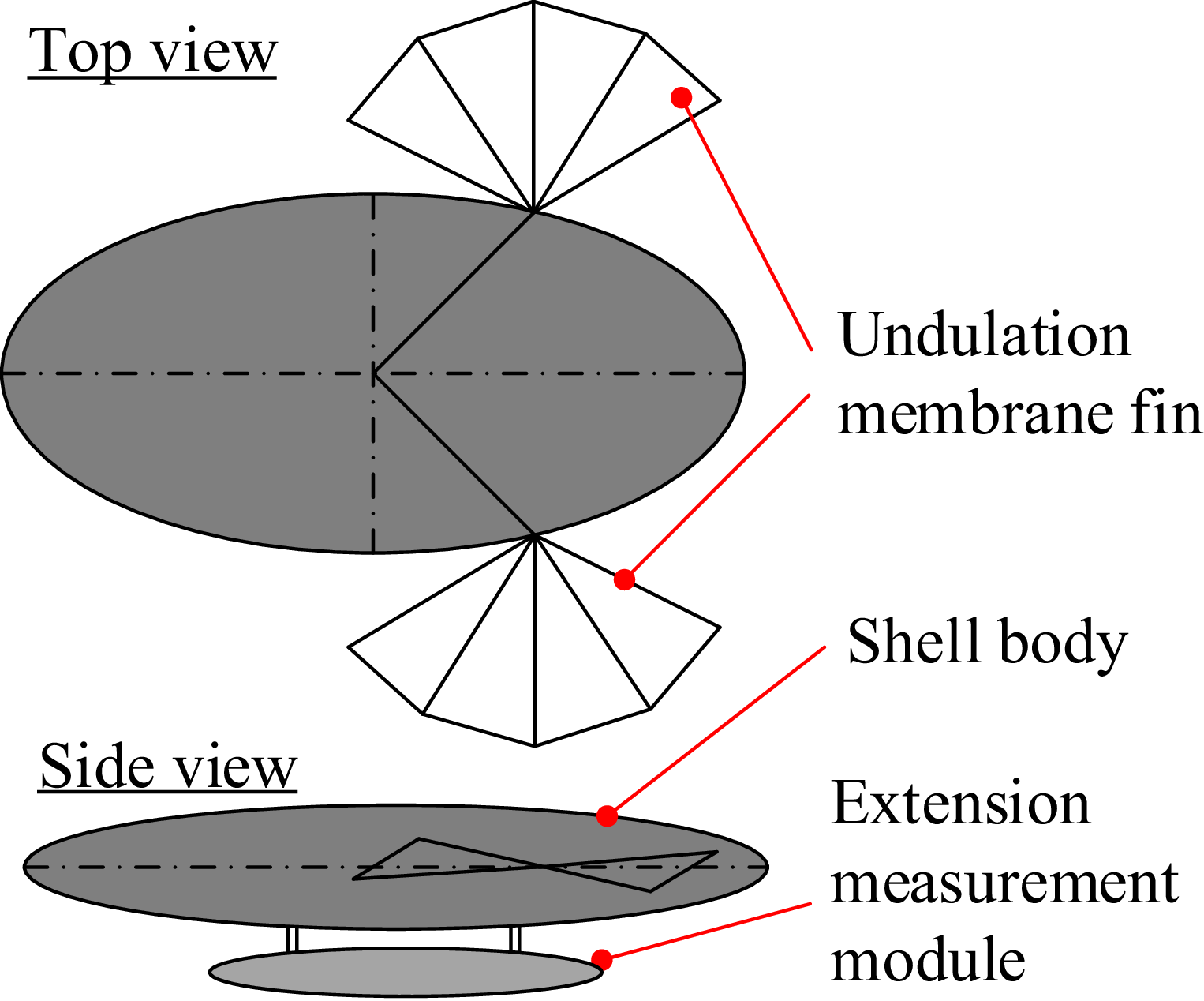
A streamlined robotic fish design employing laterally undulating pectoral fins for propulsion is presented in Figure 1. Each fin is actuated with a single degree of freedom, enabling the generation of bidirectional thrust to drive the main body in planar motion. Additionally, an expansive module can be integrated into the ventral section of the robot, mechanically coupled to the main body, for the purpose of environmental sensing or water sample collection.
Schematic diagram of the operating principle.

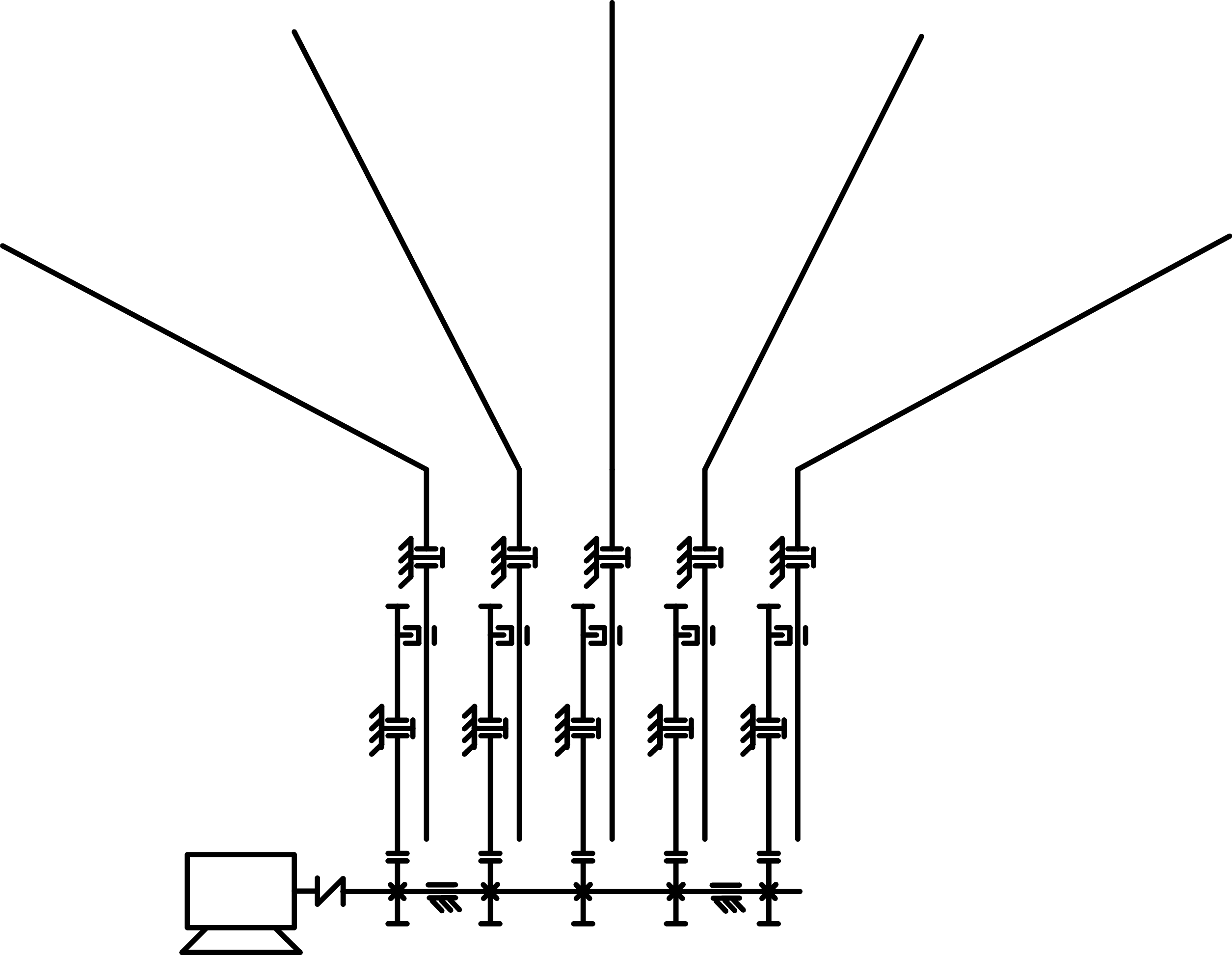
Kinematic diagram of a single-fin module.

An efficient propulsion system is essential for robotic fish. This section presents a novel modular propulsion design for the pectoral fins. The robot features two propulsion modules, symmetrically positioned on either side beneath the head, emulating the morphology of natural fish. Figure 2 depicts a propulsion module, consisting of a single motor, five gear transmission pairs, and five fin-ray crank mechanisms. A crank-slider mechanism, coupled with gear pairs, converts the motor’s rotary motion into oscillatory motion of the fin rays. The fin rays are arranged in a fan-shaped configuration, enabling a compact transmission design while allowing manual adjustment of phase angles between fin rays through angular positioning of drive gears on a shared motor-driven shaft. This setup converts rotational motion from a single motor into oscillatory motion of five compact fin rays with adjustable phase offsets.
Figure 3 presents the 3D structural model of the propulsion module, developed using a commercial computer-aided design and analysis tool (Autodesk Inventor). The module is designed as an independent unit, enabling easy and rapid attachment or detachment from the robot’s body. The motor is housed within the robot’s head for waterproofing and is connected to the module’s drive shaft via a magnetic coupling. Additionally, the fin rays can be detached from their base using a hexagonal threaded connector, facilitating robot compaction for transport. The gear reduction ratio is 21:64. The driving gears (smaller gears) can be angularly adjusted around the drive shaft to modify the phase difference between fin rays. These features enable rapid deployment, compaction, and adjustment of kinematic parameters.
Structure of the propulsion module.

Structure of the head and tail shell of the robot.

Figure 4. Long description
The image presents a cross-sectional view of a robotic fish, focusing on the head and tail shell. Panel A shows the head shell, which is a complex structure with various internal components. The outer shell is depicted in a solid, reddish-brown color, with internal compartments and support structures visible. Panel B illustrates the tail shell, which is shown in a color-coded displacement map. The tail shell is predominantly blue, indicating minimal displacement, with regions of green, yellow, and red showing increasing levels of displacement. The color scale on the right ranges from blue (0 mm) to red (1.05 mm), indicating the magnitude of displacement. The internal structure of the tail shell includes several ribs and support beams, which are integral to its function and movement.
To ensure waterproofing of the robot’s internal components, such as the motor and electrical systems, the design of the outer shell was meticulously considered. As illustrated in Figure 4, the robot’s structure comprises two primary sections: the front and rear compartments. To evaluate its structural response, finite element analysis (FEA) was conducted using a simulation tool (Autodesk Inventor). This static analysis assesses the deformation behavior of the compartments under external hydrostatic pressure. The front section houses two propulsion module chambers, fully isolated from the internal space containing the electrical circuits, motors, and counterweights. The rear section accommodates the battery, sensors, microcontroller, and external cable connectors for interfacing with optional measurement modules. Static deformation simulations under hydrostatic pressure (equivalent to a 2-meter water column) were performed to identify the weakest points in the designed shell framework. The two halves of the robot body are fastened together using 44 M3 bolts and a 5.10
 $^{-4}$
m thick silicone gasket, resulting in the robot’s overall length of 0.45 m.
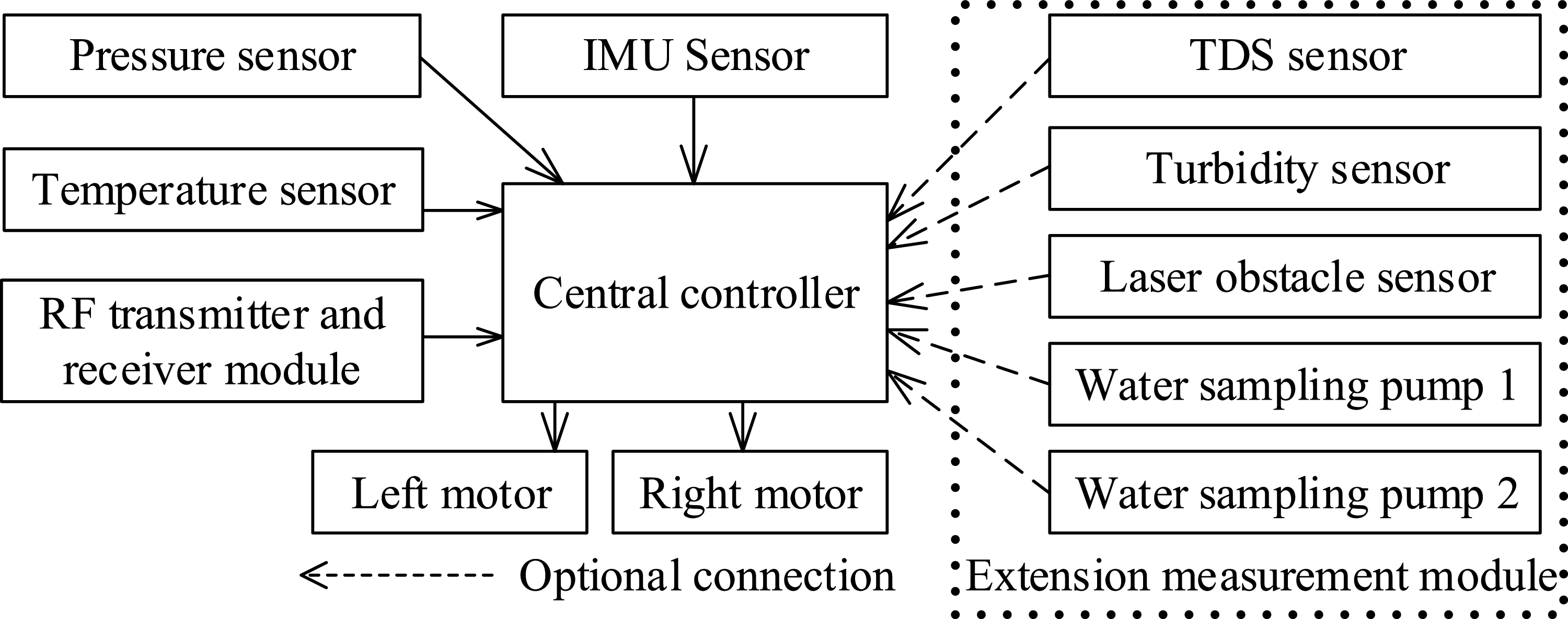
In addition to the mechanically designed hull, the electrical, control, and sensor systems were proposed. The central control unit interfaces with two motors driving the left and right fin modules, an Inertial Measurement Unit (IMU), a pressure sensor, and an RF LoRa communication module. Furthermore, a design for an optional measurement expansion module was proposed. This module incorporates two water-sampling motors, a total dissolved solids sensor, a turbidity sensor, and a laser-based obstacle detection sensor. The schematic diagram of the proposed system is presented in Figure 5.
Figure 6 illustrates the robotic fish that includes the primary subsystems as follows: two propulsive modules, a balance module, an expansive measurement module, a battery, and a control and electrical system. These parts can be disassembled easily, especially the propulsive modules that can be removed or installed immediately when the robot needs to be deployed. The design parameters, including geometric dimensions, center of buoyancy, and moment components of mass inertia, are also extracted from the design.
To estimate the position of the Center of Buoyancy (CoB) during the initial design phase, the total vehicle hull was rendered as a solid water volume within the computer-aided design (CAD) environment. Additionally, external components, such as the two fin-actuated modules, were assigned material properties equivalent to water to account for displacement. This approach allowed for an accurate determination of the CoB position.
Schematic diagram of the electrical system on the robot.

3D design model of the robot with an extended measurement module.

Figure 6. Long description
A diagram of a robotic fish design model with labeled components. Panel A: Assembly model without the shell. The diagram shows the internal structure of the robotic fish, including the CoM adjustment module, propulsive module, BLDC geared motor, pressure sensor, and Arduino mini M0. Panel B: Assembly model with the shell. The diagram shows the external structure of the robotic fish, including the fin rays and extensive measurement module.
3. Dynamic analysis
This part presents a dynamic analysis for a fish robot propelled solely by dual undulating pectoral fins. The primary aim is to establish a computational model that describes the influence of fin oscillatory motion on the swimming speed and propulsive efficiency of the robotic fish, with the motion constrained to a two-dimensional horizontal plane for analytical simplification. To facilitate the development of the mathematical model, several assumptions are adopted: the robot’s buoyancy center is aligned with its mass center in the horizontal plane projection, and its weight is calibrated to achieve neutral buoyancy. Furthermore, the robot’s body is modeled as an ellipsoid, facilitating the calculation of fluid inertia and damping impacts on the structure.
To model the motion of the robotic fish’s pectoral fins and body in a fluid medium, three coordinate systems are defined: the inertial coordinate frame, the body-fixed coordinate frame, and the pectoral fin coordinate frames, denoted as
 $O_wXYZ$
,
 $O_B x_B y_B z_B$
,
 $O_L x_L y_L z_L$
,
 $O_R x_R y_R z_R$
,
 $O_{Li} x_{Li} y_{Li} z_{Li}$
, and
 $O_{Ri}x_{Ri}y_{Ri}z_{Ri}$
, respectively (see Figure 7). The body-fixed coordinate frame is aligned with the robot’s center of buoyancy. The coordinate frames of the right and left pectoral fins are anchored at the revolute joints of the respective fin rays, with subscripts
 $R$
or
 $L$
(collectively referred to as
 $K$
in subsequent equations) indicating the right or left fin and the subscript denoting the fin ray order. A detailed schematic of these notations is provided in Figure 7. Here,
 $\psi$
represents the body’s heading angle (defined as the angle between the
 $x_B$
and
 $X$
axes), and
 $\gamma _{Ki}$
indicates the oscillation angle of a fin ray. Unit vectors for the inertial and body–referenced coordinate frames are represented as
 $[\vec {i}_W,\vec {j}_W,\vec {k}_W]$
, and
 $[\vec {i}_B,\vec {j}_B,\vec {k}_B]$
, respectively. The connection between the unit vectors of the body-fixed and inertial coordinate frameworks is detailed in Appendix (Eqs. (A1, A2, A3)).
Diagram illustrating fin motion analysis in a two-dimensional plane.

Diagram of the swing arm mechanism.

Figure 8. Long description
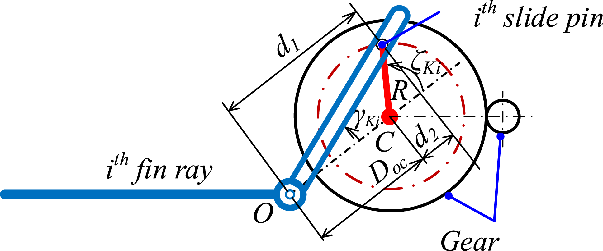
A diagram of the swing arm mechanism. The diagram shows a circular gear mechanism with labeled components. The i-th fin ray extends from point O to the gear, where it connects to a slide pin. The slide pin moves along a circular path defined by the gear’s radius R. The distance d1 represents the length from point O to the center of the gear, labeled C. The distance d2 represents the radius of the circular path along which the slide pin moves. The angle Ki is formed between the fin ray and the line connecting O to C. The angle K’i is formed between the slide pin and the line connecting C to the slide pin. The diagram illustrates the mechanical interaction between the fin ray, slide pin, and gear, demonstrating how the fin ray’s movement is translated into the slide pin’s motion along the circular path.
Second, to generate the oscillatory motion of each fin ray, a gear-driven crank and slider mechanism is employed, as depicted in Figure 8. Let
 $\zeta _{Ki}$
represent the rotational position of the motor-driven crank connected to the pivot. The symbols
 $R$
and
 $D_{oc}$
express the crank radius and the distance from the fin-ray pivots to the big gear-driven crank pivot, respectively. The association between
 $\zeta _{Li}(t)$
and the oscillation frequency
 $f_K$
of the fin ray
 $i^{th}$
on the pectoral fin
 $K$
is expressed as follows:
 $\zeta _{Li}(t) = 2\pi f_L(t) t + \phi _{\gamma Li}$
,
 $\zeta _{Ri}(t) = -2\pi f_R(t) t + \phi _{\gamma Ri}$
, where
 $f_K(t) = n_K(t)/60$
,
 $n_K$
is the crankshaft
 $K$
’s revolutions per minute, and
 $\phi _{\gamma Ki}$
represents the phase deviation between consecutive fin rays.
The angle, angular velocity, and angular acceleration of the fin ray
 $i$
belonging to the pectoral fin are computed as follows, respectively:
 \begin{equation} \gamma _{Ki} = \arctan 2\left ( {R\sin \zeta _{Ki}},{D_{oc}+R\cos \zeta _{Ki}}\right )\!, i = \overline {1,5} \end{equation}
 \begin{equation} \dot \gamma _{Ki} = \frac {-2\pi Rf_K(t)(D_{oc} \cos \zeta _{Ki}(t)+R)}{\big(D^2_{oc} + 2D_{oc}R \cos \zeta _{Ki}(t)+ R^2\big)} \end{equation}
 \begin{equation} \ddot \gamma _{Ki} = \frac {-4\pi ^2 R f_K^2(t) D_{oc} \sin \zeta _{Ki}(t)\big(D_{oc}^2 - R^2\big)}{\big(D^2_{oc} + 2D_{oc} R \cos \zeta _{Ki}(t)+ R^2\big)^2} \end{equation}
Thirdly, the motion of the robotic fish in the inertial frame can be described using the following coordinate transformation:
 \begin{equation} \begin{cases}\dot {X} = v_x \cos \psi - v_y \sin \psi , \\[5pt] \dot {Y} = v_x \sin \psi + v_y \cos \psi , \\[5pt] \dot {\psi } = \omega _z. \end{cases}\end{equation}
Here,
 $v_x$
,
 $v_y$
, and
 $\omega _z$
denote the velocities of surge, sway, and yaw motions of the body, respectively;
 $\psi$
represents the heading position, defined as the angle between the axis of the body-fixed coordinate system
 $x_B$
and the axis of the inertial frame system
 $X$
(refer to Figure 9).
Planar dynamic analysis model of the fish robot with the fan-shaped pectoral fins.

Figure 9. Long description
A diagram of a fish robot with fan-shaped pectoral fins, showing various forces and moments acting on it. The diagram includes a coordinate system with axes labeled X, Y, and Z. The fish robot is depicted with its body axis labeled xB and yB. The pectoral fins are shown on both the left (L) and right (R) sides, with forces FL and FR acting on them in the x and y directions. Moments ML and MR are also shown acting on the fins. The diagram includes labels for various forces and moments, such as fD, τD, α, and Ψ. The fish robot’s center of rotation is marked as OB. The diagram illustrates the interaction between the fish robot’s body and the surrounding water, highlighting the dynamic analysis of the robot’s movement.
Fourthly, to describe the dynamic behavior of the fish robot in the body-fixed frame, Kirchhoff’s equation is utilized [Reference Fossen38]. The robot is assumed to operate with three degrees of freedom in the horizontal plane, namely surge (
 $v_x$
), sway (
 $v_y$
), and yaw (
 $\omega _z$
). The robot’s body is symmetric about the plane
 $O_Bx_Bz_B$
, allowing the off-diagonal terms of the inertial matrix with respect to the
 $y_B$
-axis to be set to zero. As the robot operates at low speeds, inertial coupling terms among surge, sway, and yaw motions are neglected. Consequently, the resulting equation is simplified as follows:
 \begin{equation} \begin{cases}(m_b+m_x)\dot {v}_x -(m_b+m_y)v_y\omega _z = F_x \\[5pt] (m_b+m_y)\dot {v}_y +(m_b+m_x)v_x\omega _z = F_y \\[5pt] (J_b+J_z)\dot \omega _z -(m_x-m_y)v_yv_y = M_z \end{cases} \end{equation}
Where
 $m_b$
and
 $J_b$
represent the robot’s mass and its moment of inertia about the
 $z$
-axis, respectively. The terms
 $m_x$
, and
 $m_y$
denote the added mass components associated with the
 $x_B$
-axis and
 $y_B$
-axis, while
 $J_z$
symbolizes the added inertia of the robot about the
 $z_B$
-axis. Additionally,
 $F_x$
and
 $F_y$
represent the external forces in surge and sway directions, respectively, while
 $M_z$
denotes the yaw moment acting on the robotic fish body due to the pectoral fins.
The corresponding expressions are derived as follows:
 \begin{equation} F_x = F^x_R + F^x_L + f_L\sin \alpha -f_D\cos \alpha , \end{equation}
 \begin{equation} F_y = F^y_R - F^y_L - f_L\cos \alpha -f_D\sin \alpha , \end{equation}
 \begin{equation} M_z = F^x_R b_1 + F^y_R a_1 - F^x_L b_1 - F^y_L a_1 + M^z_L - M^z_R + \tau _D. \end{equation}
Here, the fluid forces acting on the robot’s mass center, denoted as
 $f_D$
,
 $f_L$
, and
 $\tau _D$
, represent the drag force, lift force, and drag moment, respectively (refer to Figure 9).
 \begin{equation} f_D = 0.5C_DS\rho _H V^2, \end{equation}
 \begin{equation} f_L = 0.5C_LS\rho _H V^2 \alpha , \end{equation}
 \begin{equation} \tau = -C_M \text{sgn}(\dot {\psi }) \dot {\psi }^2 \end{equation}
Here,
 $C_D$
,
 $C_L$
, and
 $C_M$
represent the coefficients for drag, lift, and drag moment, respectively. The terms
 $S$
and
 $\rho _H$
indicate the submerged surface area of the robot’s body and the density of the water, respectively. The robot’s linear velocity,
 $V$
, is determined by the expression
 $V = \sqrt {v^2_x+v^2_y}$
. The angle of attack
 $\alpha$
is defined as the angle between the velocity vector
 $\vec {V}$
and
 $x_B$
-axis.
Fifthly, to determine the values of
 $F^x_K$
,
 $F^y_K$
, and
 $M^z_K$
, we integrate the forces and moments produced by each fin membrane. This enables the expression of the total components relative to
 $x_K$
,
 $y_K$
, and
 $z_K$
axes for each pectoral fin, as follows:
 \begin{equation} F^x_K = \sum _{i=1}^{N-1} \left ( \left ( \vec {n}_{Ki,i+1}\;.\;\vec {i}_B\right ) .\;F_{Ki,i+1}\right )\!, \end{equation}
 \begin{equation} F^y_K = \sum _{i=1}^{N-1} \left ( \left ( \vec {n}_{Ki,i+1}\;.\;\;\vec {j}_B\right ) .\;F_{Ki,i+1}\right )\!, \end{equation}
 \begin{equation} M^z_K = \sum _{i=1}^{N-1} \big( \big ( \vec {n}_{Ki,i+1}\;.\;\vec {k}_B\big)\;.\;M_{Ki,i+1}\big). \end{equation}
It is significant to observe that
 $i$
ranges from 1 to
 $N-1$
, with
 $N=5$
indicating the total count of fin rays in a pectoral fin. The force and the moment, corresponding,
 $F_{Ki,i+1}$
,
 $M_{Ki,i+1}$
, stemming from the engagement of the surrounding fluid with the fin webbing segment enclosed by two successive fin rays, are calculated as outlined below:
 \begin{equation} F_{Ki,i+1} = \displaystyle\int _{r^{min}_{Ki,i+1}}^{r^{max}_{Ki,i+1}} dF_{Ki,i+1}(r_{Ki,i+1},t), \end{equation}
 \begin{equation} M_{Ki,i+1} = \displaystyle\int _{r^{min}_{Ki,i+1}}^{r^{max}_{Ki,i+1}} r_{r_{i,i+1}}dF_{Ki,i+1} (r_{Ki,i+1},t). \end{equation}
Where,
 \begin{equation} {r^{max}_{Ki,i+1}} = \left ( L_0+L\right ) \cos {\frac {\lambda _{Ki,i+1}}{2}}, \end{equation}
 \begin{equation} {r^{min}_{Ki,i+1}} = L_0\cos {\frac {\lambda _{Ki,i+1}}{2}}. \end{equation}
A geometric depiction of a fin webbing enclosed by two successive fin rays is illustrated in Figure 10. To assess the external load applied to each unit length of a fin webbing segment, Morison’s hydrodynamic model is employed, with calculations as follows:
 \begin{equation} \begin{aligned} dF_{Ki,i+1} ( r_{Ki,i+1},t) &= -C_a \frac {\pi }{4} \rho _H d^2_{Ki,i+1} a_{Ki,i+1} ( r_{Ki,i+1},t) dr_{Ki,i+1} \\ &\quad - \frac {1}{2} C_d d_{Ki,i+1} \rho _H v_{Ki,i+1} ( r_{Ki,i+1},t) \left | v_{Ki,i+1} ( r_{Ki,i+1},t) \right | dr_{Ki,i+1}, \end{aligned} \end{equation}
where,
 \begin{equation} {r_{Ki,i+1}} = s_{Ki,i+1}\cos {\frac {\lambda _{Ki,i+1}}{2}}, \end{equation}
 \begin{equation} d_{Ki,i+1} =2 r_{Ki,i+1} \tan {\frac {\lambda _{Ki,i+1}}{2}}. \end{equation}
Here,
 $C_a$
,
 $C_d$
denote the coefficients representing the inertial and damping effects of fluid flow, respectively. The terms
 $a_{Ki,i+1}$
and
 $v_{Ki,i+1}$
indicate the acceleration and velocity of the segment center bounded by the
 $i^{th}$
and the
 $\left (i+1\right ) ^{th}$
fin ray (see Figure 10), with their magnitudes determined as follows:
 $a_{Ki,i+1} = ^W\mspace {-5mu}\ddot {\vec {p}}_{Ki,i+1}^T \vec {n}_{Ki,i+1}$
,
 $v_{Ki,i+1} = ^W\mspace {-5mu}\dot {\vec {p}}_{Ki,i+1}^T \vec {n}_{Ki,i+1}$
, here,
 $\vec {p}_{Ki} = P_{Ki}-P_{Ki}^0$
;
 $P_{Ki}^0$
, and
 $P_{Ki}$
represent the coordinates of a point
 $s_{Ki,i+1} = L_0$
fin ray and a point
 $L_0 \lt s _{Ki,i+1} \leqslant L_0+L$
on the
 $i^{th}$
fin ray, respectively, of the pectoral fin
 $K$
(refer to Figure 10). To obtain the position coordinates of any point on the fin ray with respect to the inertial coordinate system, equations from Eqs. (A4) to (A15) in the Appendix are employed.
Geometric representation of two fin webbing bounded by three sequential fin rays.

Furthermore,
 $\vec {n}_{Ki,i+1}$
represents the normal vector of the plane defined by the
 $i^{th}$
and
 $\left ( i+1\right ) ^{th}$
fin rays, calculated as
 $ \vec {n}_{Ki,i+1} = \vec {p}_{Ki} \times \vec {p}_{Ki+1}$
, where the operator “
 $ \times$
” signifies the cross-product of two vectors.
It is observed that the angle formed between two successive fin rays, constrained within the range of 0 to
 $ \pi /4$
radians, can be determined using the subsequent formula:
 \begin{equation} \lambda _{Ki,i+1} = \cos ^{-1} \left ( \frac {\vec {p}_{Ki}\;.\;\vec {p}_{Ki+1}}{\parallel \vec {p}_{Ki}\parallel . \parallel \vec {p}_{Ki+1}\parallel } \right ) \end{equation}
By consolidating Eqs. (20, 21), and (22) into Eq. (19) and merging them with Eqs. (15, 16), a collection of differential equations can be constructed to model the robot’s movement within the inertial reference framework (Eq. (5)). In this structure, the rotational rates of the motor shafts function as the driving variables. To evaluate the mechanical performance of the robot’s movement, the subsequent formula is applied:
 \begin{equation} \eta = \frac {\int _{0}^{T} P_{out}\left ( t\right ) dt}{\int _{0}^{T} P_{in}\left ( t\right ) dt} , \end{equation}
Here,
 $T$
signifies the testing timeframe, whereas
 $ P_{out}\left ( t\right )$
and
 $ P_{in}\left ( t\right )$
indicate the produced and supplied power, respectively, resulting from the function of the pectoral fins. These formulations are calculated as outlined below:
 \begin{equation} P_{out}\left ( t\right ) = f_D v_x , \end{equation}
 \begin{equation} \begin{aligned} P_{in}(t ) &= -( ( F_{xR} + F_{xL} ) v_x + ( F_{yR} + F_{yL} ) v_y ) \\ &\quad-( ( ( F_{xR} + F_{xL}) b_1 + ( F_{yR}+F_{yL} ) a_1 + M_{zR} + M_{zL} ) \omega _z ). \end{aligned} \end{equation}
The useful propulsive power is indirectly calculated based on the drag force generated by the fluid [Reference Suzuki, Kato and Suzumori37]. The mechanical efficiency provides a means to evaluate the robot’s energy utilization behavior and the effectiveness of the suggested fin configuration. To evaluate the quality of forward velocity performance of the robot, we apply the ripper factor in the steady state of robot motion that is defined as follows:
 \begin{equation} \gamma = \frac {v_{x,RMS}}{v_{x,a}} 100 \% \end{equation}
Where
 $v_{x,a}$
is the average value of the forward velocity of the robot in steady state time, determined by:
 \begin{equation} v_{x,a} = \frac {1}{T_S} \int _{t_{fm}-T_S}^{t_{fm}} {v_{x}}\left ( t\right ) dt \end{equation}
 \begin{equation} v_{x,RMS} = \sqrt {\frac {1}{T_S} \int _{t_{fm}-T_S}^{t_{fm}} ({v_{x}}\left ( t\right ) -v_{x,a}) ^2 dt} \end{equation}
Here,
 $t_{fm}$
and
 $T_S$
denote the final measurement time and the selected testing time, respectively.
4. Fabrication and experimental setup
In this section, the results of the fabrication of the modules are presented. Initially, the left and right propulsion modules are introduced. Subsequently, the fabrication of the structural frame is described. The installation and arrangement of motors and sensors are detailed comprehensively. Finally, several configurations for experimental testing and trial runs of the model are outlined. The process of testing with the expanded measurement module is also conducted. To realize the proposed designs, the fabrication of modules and experimental trials were conducted. Initially, the left and right propulsion modules were constructed. To achieve lightweight and rigid structural walls, the partition plates were fabricated using fused deposition modeling (FDM) 3D printing with polyethylene terephthalate glycol (PETG) filament, followed by a vacuum-assisted LRAB21H epoxy resin coating. These fabricated partitions were subsequently secured and aligned using four 8-mm-diameter aluminum rods, which were rigidly connected to the plates via M3 hexagonal socket screws to ensure structural integrity. The rotating shafts supporting the fin rays and the primary drive shaft, with corresponding diameters of 6 mm and 4 mm, were made of 304 stainless steel. Similarly, the five fin ray bases were also fabricated from stainless steel to mitigate oxidation in aqueous environments. Each fin ray base consisted of a 12 mm outer diameter stainless steel tube combined with a 4 mm stainless steel arm through a brazed joint. Additionally, two flanged ball bearings were employed for each fin ray base to ensure coaxial motion and reduce friction. The primary drive shaft, fitted with small gears, was constrained in five degrees of freedom using brass bearings to minimize friction. The spacing between the fin ray bases was achieved using thin stainless steel washers. A detailed illustration of this module is presented in Figure 11. To facilitate the assembly and disassembly of the fin membrane, the fin rays were manufactured as separate components, connected to the fin ray bases using threaded coupling nuts.
Validation results of the TDS sensor.

Table I. Long description
A table comparing TDS pen measurements with a robot’s TDS module across six samples. The table has 6 rows and 3 columns. Column headers are No. sample, TDS pen, and The robot’s TDS module (mean ± standard deviation (SD)). Row labels are 1, 2, 3, 4, 5, and 6. Row 1: No. sample 1, TDS pen 111, The robot’s TDS module (mean 127.13 ± standard deviation (SD)) 0.92. Row 2: No. sample 2, TDS pen 162, The robot’s TDS module (mean 166.53 ± standard deviation (SD)) 1.13. Row 3: No. sample 3, TDS pen 206, The robot’s TDS module (mean 204.68 ± standard deviation (SD)) 1.32. Row 4: No. sample 4, TDS pen 428, The robot’s TDS module (mean 404.91 ± standard deviation (SD)) 0.97. Row 5: No. sample 5, TDS pen 621, The robot’s TDS module (mean 566.22 ± standard deviation (SD)) 1.42. Row 6: No. sample 6, TDS pen 744, The robot’s TDS module (mean 649.38 ± standard deviation (SD)) 4.23.
Illustration of the fabricated propulsive module.

Figure 11. Long description
A diagram of a fabricated propulsive module with labeled components. The diagram includes a driven gear, fin tip base, solid bronze flanged bushings, slide pin on gear, permanent magnet coupling, driving gear, and frame fixing bars. The driven gear is located at the top left, while the fin tip base is positioned centrally. Solid bronze flanged bushings are distributed along the central axis. The slide pin on gear is situated near the driven gear. The permanent magnet coupling is located at the bottom left, adjacent to the active bear. Frame fixing bars are positioned at the bottom right, supporting the structure.
To prevent water ingress into the robot’s body while ensuring the transmission of rotational motion from the motor to the propulsion module, a magnetic coupling design was implemented. Each side of the coupling utilized ten
 $10 \times 5 \times 3 \text{ mm}^3$
permanent magnets arranged in an alternating polarity fan configuration to enhance coupling strength [Reference Shin, Choi, Jang and Lim39]. The water-sealing partition between the two coupling halves was constructed from 0.2 mm thick stainless steel. For the propulsion system, a BLDC M2006 motor and a C610 RobotMaster controller were employed due to their compact size and high torque output. The robot was equipped with an Arduino M0 mini microcontroller, a Gravity-Analog water pressure sensor, a 10 DOF IMU sensor (Waveshare), and an INA226 voltage, current, and power consumption sensor. Additionally, the robot incorporated a LoRa Lora HAT SX126X 443 MHz wireless communication module. This module was selected for its long-range transmission capabilities and superior data transfer efficiency from aquatic to aerial environments, facilitated by an antenna, compared to high-frequency RF alternatives.
To achieve a neutral buoyancy state, counterweights were added through an iterative, step-by-step process. The horizontal balance (the alignment of the Center of Mass (CoM) and CoB) was then refined by adjusting the positions of these weights. Specifically, the robot was equipped with a dedicated CoM adjustment module featuring small counterweights, allowing for precise and convenient post-assembly tuning (see Figure 6).
Subsequently, additional components were fabricated via FDM 3D printing, with the two halves of the shell constituting the largest PETG-printed parts. To enhance their structural integrity, these shell components were externally laminated with a carbon fiber fabric layer through a vacuum-assisted epoxy bonding process. Meanwhile, to facilitate smooth fin tip motion, the fin membrane was fabricated from approximately 0.1-mm-thick polyvinyl chloride (PVC) sheets. The resulting four distinct fin configurations, corresponding to the four phase-difference scenarios, are illustrated in Figure 12.
Furthermore, to monitor environmental parameters, a DS18B20 temperature sensor is mounted on the underside of the robot’s rear body. The external module comprises an analog turbidity sensor, an analog TDS sensor (DFRobot), a VL53L0X laser rangefinder, and an MPS20N0040D-S pressure sensor. This module is mechanically and electrically integrated with the main robotic fuselage to facilitate both environmental data acquisition and water sampling pump actuation. Notably, the ranging performance of the laser sensor undergoes significant attenuation underwater, demonstrating a high susceptibility to water turbidity. Figure 13 illustrates the complete experimental setup.
During the sensor calibration process for TDS and turbidity, the scaling coefficients for both sensors were configured based on the manufacturer reference source codes. The accuracy of the TDS sensor was subsequently validated against a commercial reference device (Xiaomi TDS pen, model: XMTDS01YM) using six distinct water samples. The validation results, summarized in Table I, demonstrate acceptable agreement with the reference device. Regarding the turbidity sensor, due to the unavailability of an industrial-grade turbidimeter for direct cross-referencing, the system relied solely on the manufacturer’s protocol and a pure water baseline. Consequently, the turbidity and TDS measurements in this study are utilized primarily to evaluate relative environmental trends rather than absolute values.
Four types of ribbon fins corresponding to the four distinct phases of fin kinematics used in the experiments.

Experimental illustration of the robotic fish with the expansive measuring device.

To regulate the speed of the motor
 $K$
to the desired value (where the subscript
 $K \in \{L, R\}$
represents the left or right side, respectively), a discrete-time PID control law is applied. The control current applied to the motors through the C610 driver at the
 $j$
-th time step is expressed as follows:
 \begin{equation} I_K(\,j)=K_pe_K(\,j)+K_i ei_K(\,j)+K_ded_K(\,j), \end{equation}
where
 $K_p$
,
 $K_i$
, and
 $K_d$
represent the proportional, integral, and derivative gains of the motor controllers, respectively (with the sampling time of 0.01 s implicitly integrated into
 $K_i$
and
 $K_d$
). The terms
 $e_K$
,
 $ei_K$
, and
 $ed_K$
denote the tracking error, the accumulated error, and the error derivative of the motor
 $K$
, which are defined as follows:
 \begin{equation} \begin{cases}e_K(\,j) = n^m_{dK}(\,j) - n^m_{K}(\,j), \\ ei_K(\,j) = ei_K(\,j-1) + e_K(\,j), \\ ed_K(\,j) = e_K(\,j) - e_K(\,j-1), \end{cases} \end{equation}
where
 $n^m_{dK}(\,j)$
and
 $n^m_{K}(\,j)$
are the desired and actual speeds of the motor
 $K$
at time step
 $j$
, respectively.
To ensure computational efficiency for the PID controller, which is configured with gains of
 $K_p = 0.55$
,
 $K_i = 0.12$
, and
 $K_d = 0.005$
, while maintaining reliable data transmission via the LoRa module (9600 baud), the experimental protocol specified a speed error sampling interval of 0.1 s, with each trial replicated three times. Detailed experimental results are discussed comprehensively in the subsequent section.
Mean speed error response of the M2006 motors.

An artificial rectangular water tank, INTEX 2282L (
 $2.60\text{ m} \times 1.60\text{ m} \times 0.65\text{ m}$
), was utilized to test the swimming performance of the robot. A high-speed digital camera, Casio Exilim EX-ZR1000, was employed to capture the robot’s movements in pixel coordinates at a speed of 30 frames/second (see Figure 13). Initially, the camera was calibrated using an
 $8 \times 7$
checkerboard (with a grid size of
 $0.05\text{ m} \times 0.05\text{ m}$
) to determine the intrinsic parameters and distortion coefficients. The recorded video was processed to identify the coordinates of red and blue marker points, which were subsequently converted to a millimeter-based coordinate system. The distance between the two identified points on the robot’s body in the millimeter coordinate system was recalculated to verify the accuracy of the transformation from pixel to real-world coordinates, minimizing errors. Finally, the robot’s center point coordinates, velocity, orientation, and turning radius were computed in the millimeter coordinate system. To mitigate random errors and ensure repeatability for each scenario, three independent trials were conducted for straight swimming and six for turning maneuvers (three each for left and right). Similarly, to reduce the effects of disturbances introduced during the image acquisition process, a 5-point moving average filter was applied to the post-processed motion data. This filter had a negligible impact on the analysis of dynamic swimming behaviors, as the resulting time lag of approximately 0.17 s is considered insignificant for offline evaluation.
5. Results and discussion
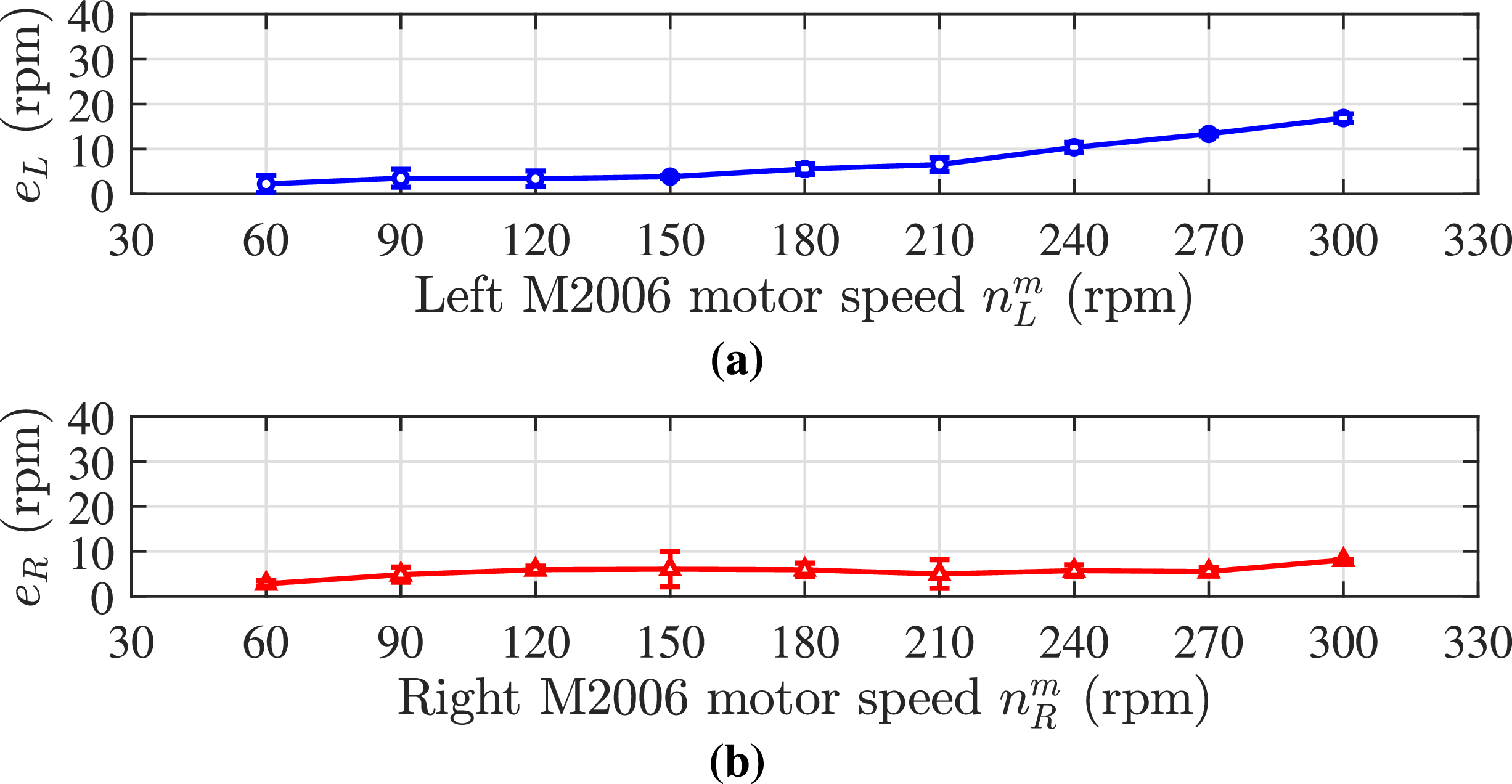
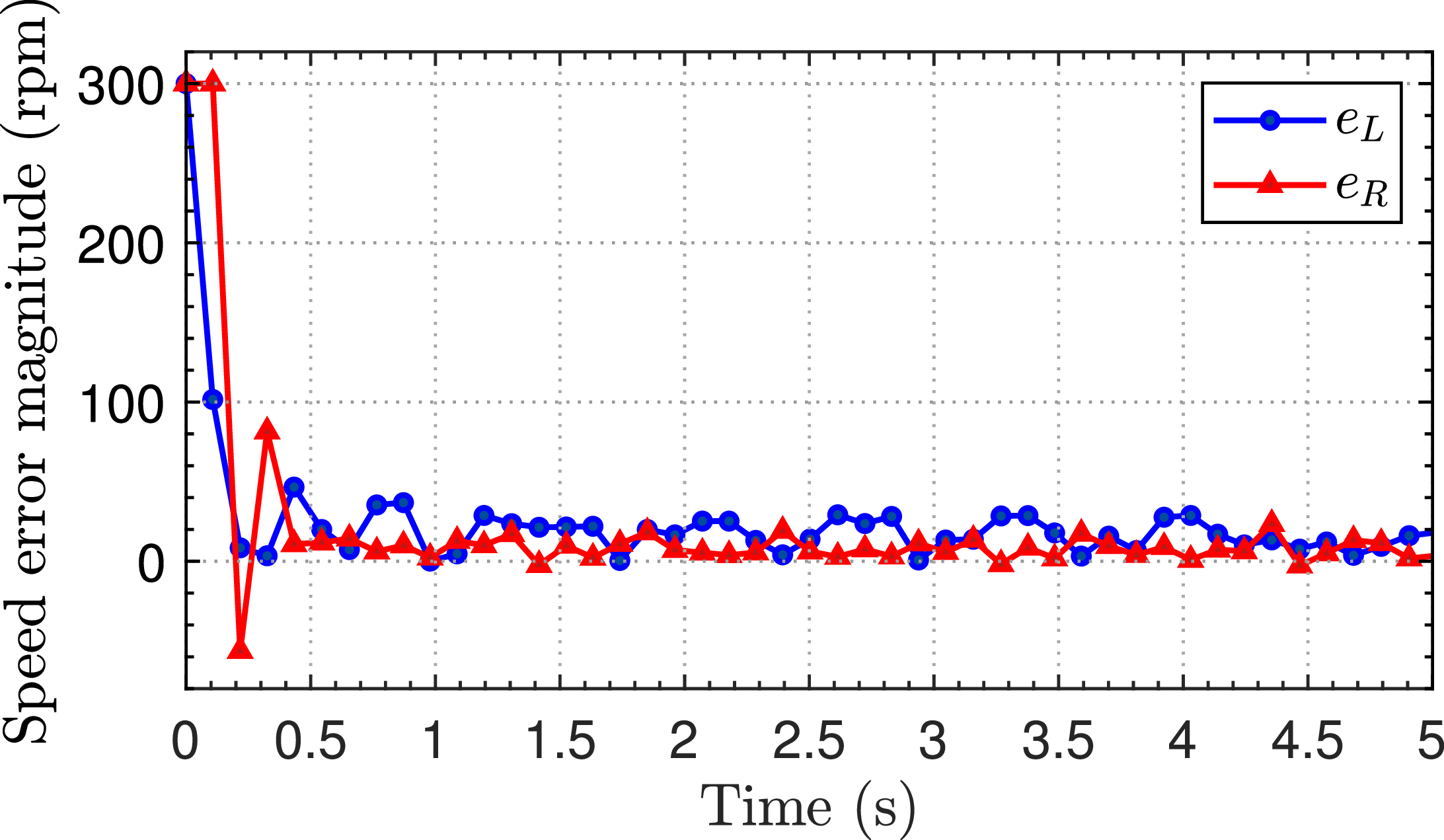
In this section, we present the simulation and experimental results. First, the speed tracking precision is presented in Figure 14. The experimental data were captured during straight-line swimming with an angle
 $\phi _{\gamma _{Li}} = -\phi _{\gamma _{Ri}} = 61.9^\circ$
. Despite the uncertainties in hydrodynamic loading, the steady-state mean errors for both the left and right motors remain remarkably small relative to their reference values, with the highest deviation staying below 6
 $\%$
. To further evaluate the transient stability of the proposed system, Figure 15 illustrates the dynamic response of the motors at a desired velocity of 300 rpm. The system achieves a settling time of approximately 0.4 s. Consequently, this PID control scheme is well-suited for evaluating the direct effects of fin actuation speed on overall swimming performance.
Speed error response of the motor
 $n^m_K$
under load at 300 rpm.

Experimental steady-state mean forward velocity of the robot during straight swimming.

Figure 16. Long description
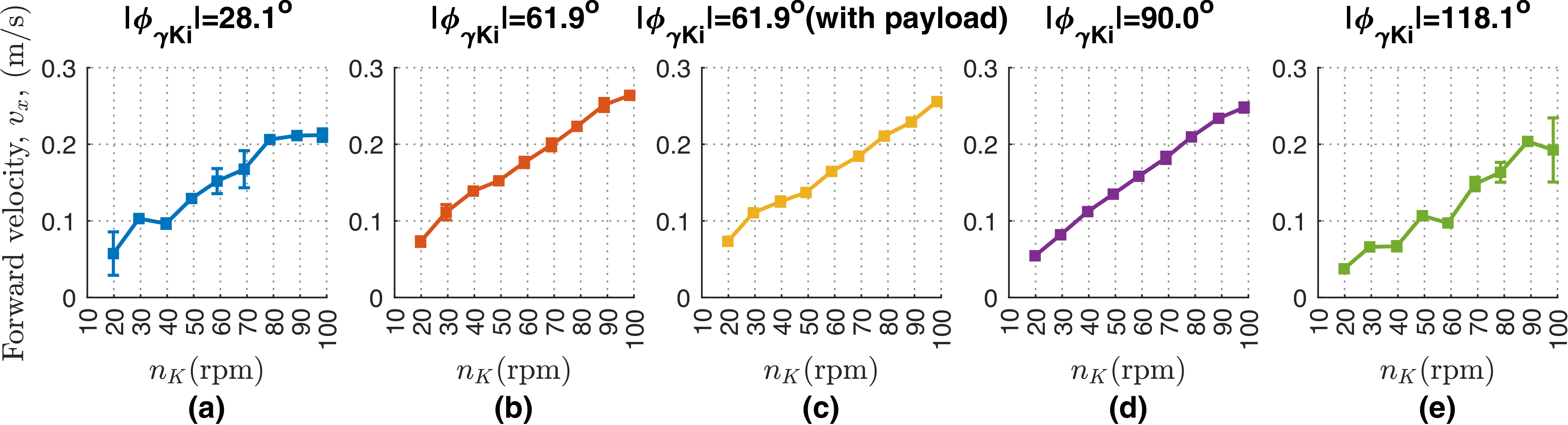
Five line graphs depict the forward velocity of a robot during straight swimming at different angles and conditions. Each graph shows the forward velocity in meters per second (m/s) on the vertical axis and the rotational speed in revolutions per minute (rpm) on the horizontal axis. Panel A: The graph shows the forward velocity at an angle of 28.1 degrees. The forward velocity increases with the rotational speed, ranging from approximately 0.05 m/s to 0.25 m/s. Panel B: The graph shows the forward velocity at an angle of 61.9 degrees. The forward velocity increases with the rotational speed, ranging from approximately 0.05 m/s to 0.25 m/s. Panel C: The graph shows the forward velocity at an angle of 61.9 degrees with a payload. The forward velocity increases with the rotational speed, ranging from approximately 0.05 m/s to 0.25 m/s. Panel D: The graph shows the forward velocity at an angle of 90.0 degrees. The forward velocity increases with the rotational speed, ranging from approximately 0.05 m/s to 0.25 m/s. Panel E: The graph shows the forward velocity at an angle of 118.1 degrees. The forward velocity increases with the rotational speed, ranging from approximately 0.05 m/s to 0.25 m/s.
Experimental steady-state mean forward velocity of the robot during turning.

Experimental mean turning radius of the robot.

Figure 18. Long description
Five line graphs depict the turning radius of a robot under different conditions. Each graph shows the turning radius in meters on the vertical axis and the rotational speed in revolutions per minute (rpm) on the horizontal axis. Panel A: The graph shows the turning radius for an angle of 28.1 degrees. The data points are represented in blue and show a relatively stable turning radius around 0.1 to 0.2 meters across different speeds. Panel B: The graph shows the turning radius for an angle of 61.9 degrees. The data points are represented in orange and show a turning radius ranging from 0.1 to 0.3 meters, with some variation across different speeds. Panel C: The graph shows the turning radius for an angle of 61.9 degrees with a payload. The data points are represented in yellow and show a turning radius ranging from 0.1 to 0.3 meters, with some variation across different speeds. Panel D: The graph shows the turning radius for an angle of 90 degrees. The data points are represented in purple and show a turning radius ranging from 0.1 to 0.3 meters, with some variation across different speeds. Panel E: The graph shows the turning radius for an angle of 118.1 degrees. The data points are represented in green and show a turning radius ranging from 0.1 to 0.2 meters, with some variation across different speeds.
The involving coefficient of the robot.

Table II. Long description
A table with two columns labeled Parameters and Value, each containing various measurements and specifications for a robot. The table has 20 rows, with each row providing a specific parameter and its corresponding value. The parameters include dimensions in meters, masses in kilograms, moments of inertia in kilogram-square meters, and angles in degrees. The values are listed in the right column, providing detailed specifications for the robot’s components and characteristics.
Next, to investigate the impacts of the phase difference between the ray fins
 $\phi _{\gamma _{Ki}}$
and the motor speed
 $n^m_K$
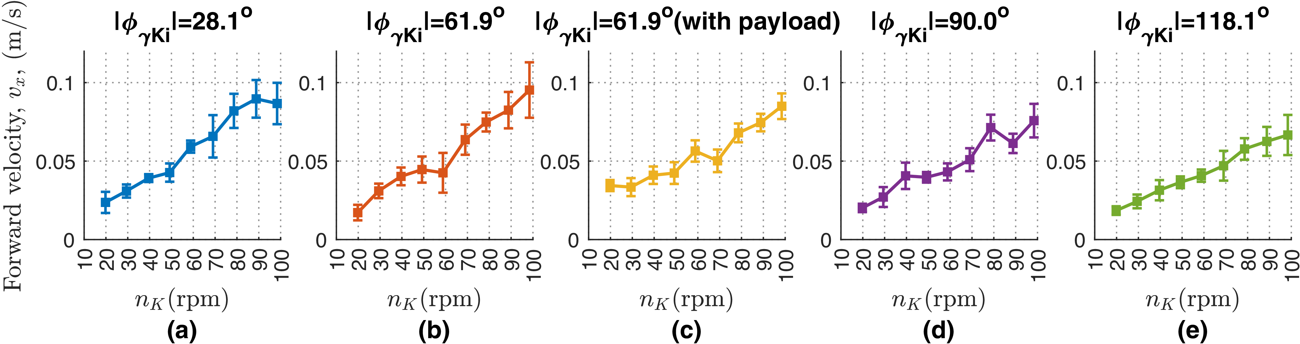
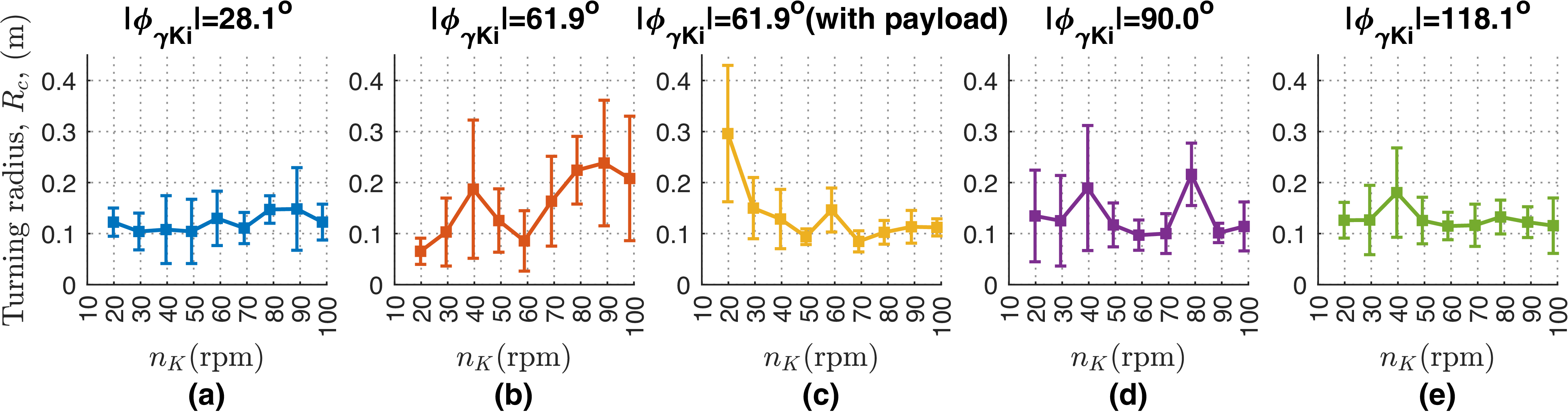
on the steady-state swimming velocity and turning performance, a series of experiments was conducted (as illustrated in Figures (16, 17, 18)). Four distinct phase differences – specifically
 $28.2^\circ$
,
 $61.9^\circ$
,
 $90^\circ$
, and
 $118.1^\circ$
– were evaluated. These values were selected as practical approximations of the nominal angles (
 $30^\circ$
,
 $60^\circ$
,
 $90^\circ$
, and
 $120^\circ$
). The motor speed ranged from 60 to 300 rpm in increments of 30 rpm, corresponding to a fin actuation speed
 $n_K$
of 19.7 to 98.4 rpm via a 21:64 gear ratio. As demonstrated in Figure 16, the robot’s velocity generally scaled with
 $n_K$
, peaking at the highest tested speed (
 $n_K = 98.4\text{ rpm}$
) under a phase difference of
 $\lvert \phi _{\gamma _{Ki}}\rvert = 61.9^\circ$
. Furthermore, to evaluate the effect of the payload (i.e., the integrated measuring module), the swimming response was analyzed. As depicted in Figure 16c, the locomotion performance exhibited a slight degradation, primarily attributed to the hydrodynamic drag induced by the additional measurement module. Importantly, the forward velocities at
 $\lvert \phi _{\gamma _{Ki}}\rvert = 28.2^\circ$
and
 $118.1^\circ$
were significantly lower than those observed in the remaining two cases. This discrepancy is likely attributable to the non-optimal fin ribbon kinematics, which compromises hydrodynamic efficiency under these specific phase relations. Additionally, the corresponding turning characteristics derived from these phase differences are detailed in Figures 17 and 18. Similar to the forward swimming trends, the robot achieved the highest turning velocity at
 $\lvert \phi _{\gamma _{Ki}}\rvert = 61.9^\circ$
; however, this peak value was significantly attenuated upon attaching the payload. Although the turning radius varied with different
 $\phi _{\gamma _{Ki}}$
configurations, no consistent trend was observed. Notably, the standard deviations of the turning radius responses were relatively large. This high variability indicates that hydrodynamic interactions and dynamic fluctuations exerted a substantial effect on the robot’s body during turning maneuvers.
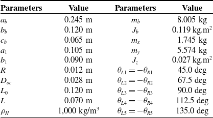
Key design and fabrication parameters related to the physical characteristics of the robot’s body and fins, which were utilized in the simulation of the proposed model, are summarized in Table II. To simplify the estimation of the added masses
 $m_x, m_y$
and the added moment of inertia
 $J_z$
, the robot’s body shape is approximated as a prolate ellipsoid [Reference Fossen38] with semi-axes
 $a_b$
and
 $(b_b+c_b)/2$
. The corresponding analytical formulas are provided in the Appendix. Some other coefficients are explained in detail. Certain hydrodynamic coefficients are estimated by integrating simulation and experimental data. Various approaches exist for determining these parameters. CFD simulations [Reference Ji, Rehman, Ajwad, Shahani, Sharma, Sutton, li, Ye, Zhu and Zhu40, Reference Xie, Zhang, Shen, Li and Zhou41] require significant computational resources but struggle to replicate real-world conditions fully. Conversely, empirical approaches [Reference Avila and Adamowski42] are effective, yielding values closely aligned with reality. In the context of undulating pectoral fins, a hybrid method combining experimental and simulation data at multiple stages is employed to sequentially determine the parameters. In step 1, we utilize analytical approximations to calculate the drag and drag moment coefficients
 $C_D$
,
 $C_M$
based on the geometric factors of an ellipsoidal robot body approximation, and a swimming speed range from 0.05 m/s to 0.30 m/s with an attack angle tolerance of
 $\pm 10^\circ$
. The obtained values of
 $C_D$
,
 $C_M$
are, respectively, 0.18 and 0.05 [Reference Sanjeevi, Dietiker and Padding43]. In the second step, the remaining coefficients, namely
 $C_L$
,
 $C_a$
, and
 $C_d$
, are adjusted by fitting the simulation results with experimental data for both forward swimming and turning maneuvers. Empirical data with
 $\lvert \phi _{\gamma _{Ki}}\rvert = 61.9^{\circ }$
(no payload) were chosen because in this case, the robot achieved the best speed performance. The corresponding fitted values were determined to be 20.5, 1, and 482. It should be noted that
 $C_d$
is much larger than
 $C_a$
, which may account for the dominant influence of drag force compared to lift force on the pectoral fins in the low-speed regime. To ensure the accuracy of the simulations, the sampling time was set to 0.001 s.
Comparison of transient forward velocities in straight swimming (
 $n_K = 98.4$
(rpm)).

Swimming trajectory and position of the robot every 0.5 s.

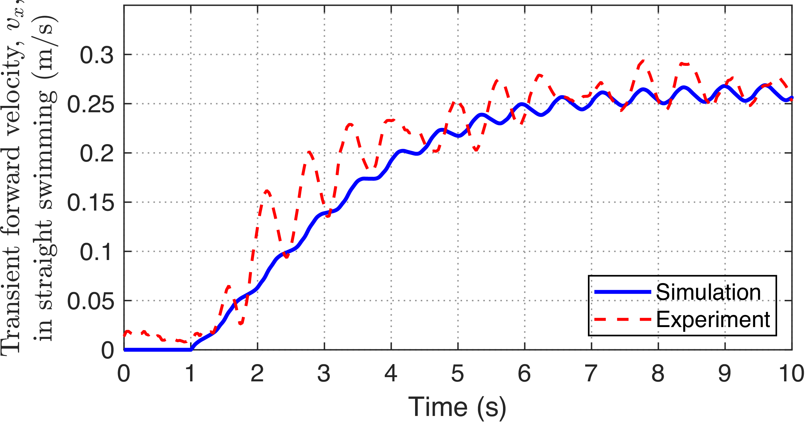
To verify the similarity between the simulation and empirical performances, the corresponding forward swimming velocities are illustrated in Figure 19. In this case, the parameters of phase difference between fin rays are chosen as
 $\phi _{\gamma Li} = 61.9^\circ$
,
 $\phi _{\gamma Ri} = -61.9^\circ$
(
 $i=1$
to 5), and the speed
 $n_K = 98.4$
rpm (approximating to the oscillatory frequency of fin ray 1.64 Hz). The forward velocity of the robot is about 0.264 m/s. The transient responses of the forward velocity obtained from the simulation and experiment are in good agreement. The more pronounced chatter phenomenon observed in the experimental results compared to the simulation may be attributed to water waves reflecting from the pool walls. To clarify the experimental data, Figure 20 shows the actual motion trajectory of the robot in free forward swimming mode, where the yellow line represents the trajectory of the robot’s center, and the red dots indicate positional points at 0.5 s intervals.
In the turning swimming mode, the robot uses only a pectoral fin to change its heading angle while maintaining linear velocity. The robot achieved 0.086 m/s and over 0.172 m/s in the experiment and simulation responses, respectively, as illustrated in Figure 21a. It is noted that the phase difference between fins was
 $\phi _{\gamma Ri} = -61.9^\circ$
, and the oscillatory frequency was 1.64 Hz. The experimental and simulation radii were 0.136 m and 0.277 m, respectively. The discrepancies in velocity and turning trajectory responses between the simulation and experimental cases can be attributed to the robot’s angle of attack, which depends on the top shape of the body’s head, leading to variable velocity and an irregular turning radius. Furthermore, Figure 21b indicates a qualitative agreement between the simulated and experimental turning performances. For a clearer visualization, Figure 22 depicts the motion trajectory trace (yellow curve) and the robot’s position every 0.5 s (red dots).
Comparison of transient forward velocities in turning swimming (
 $n_K = 98.4$
(rpm)).

Trajectory trace (yellow curve) and position every 0.5 s (red dots) of the robot motion.

Figure 22. Long description
A diagram showing the trajectory of a manta ray-inspired robotic fish. The diagram includes a blue grid background with a scale marker indicating 0.1 meters. A black robotic fish with two circular markers, one red and one green, is depicted. The yellow curve represents the midpoint trajectory of the robot, while red dots indicate the robot’s position every 0.5 seconds. The red and green dashed lines show the trajectories of the red and green markers, respectively. The diagram also includes time markers along the yellow curve, ranging from 2.05 seconds to 5.0 seconds.
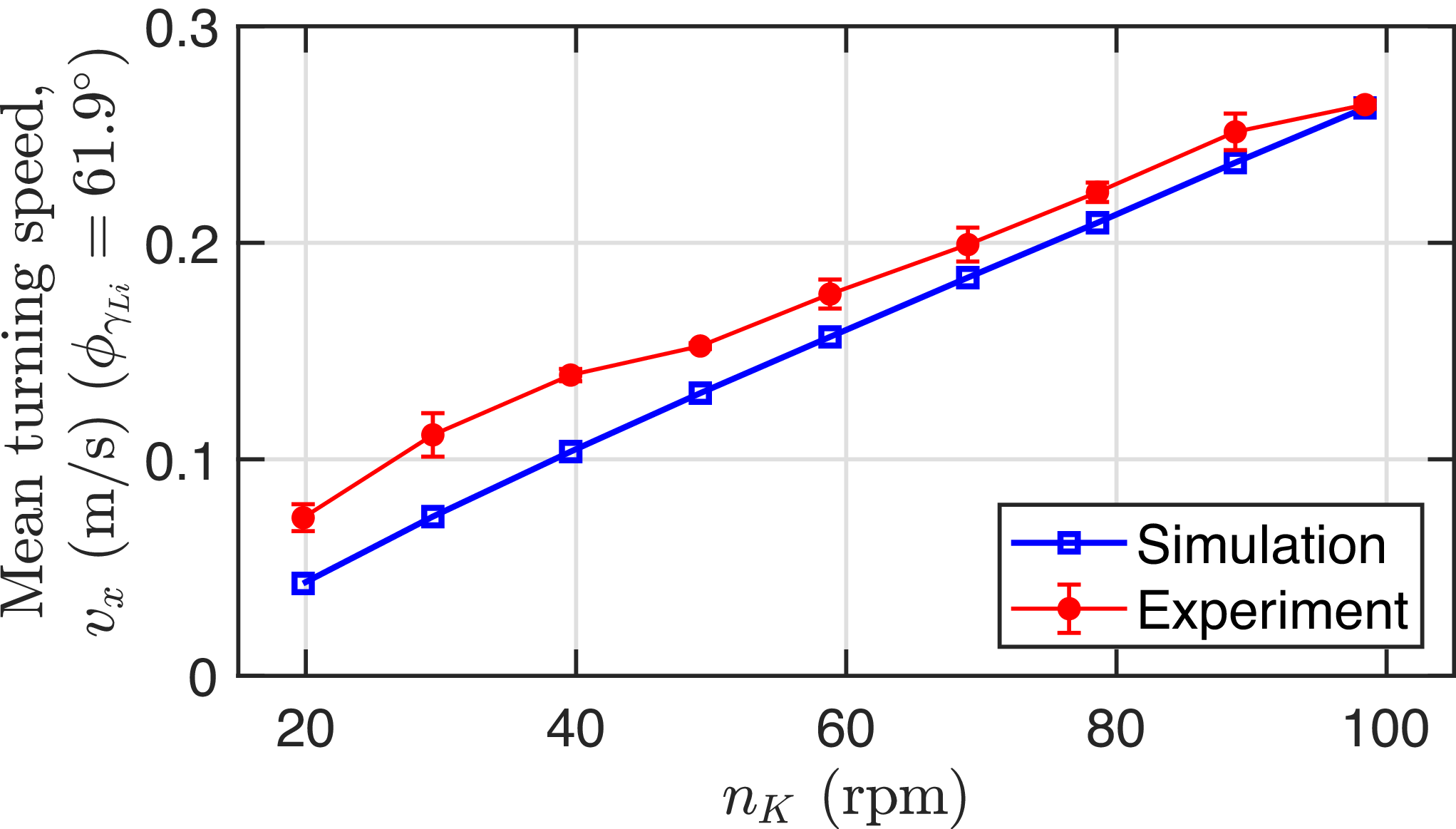
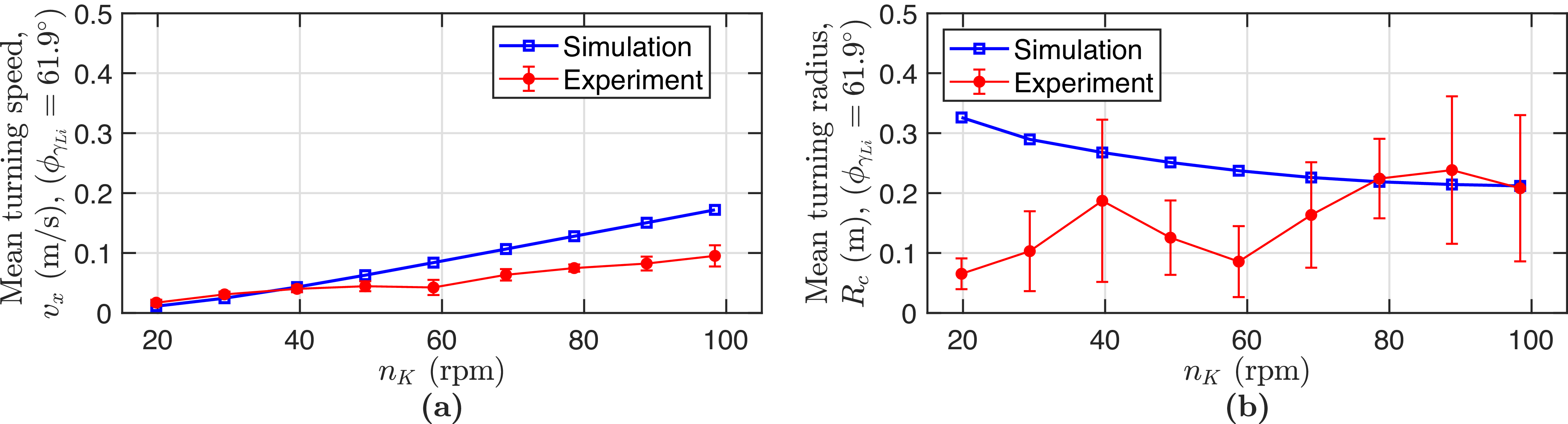
To clarify the dynamic behavior between the proposed model and experimental trials in the steady-state phase, a comprehensive comparison was conducted, as illustrated in Figures 23 and 24. It should be noted that the robot’s kinematics were configured with
 $\lvert \phi _{\gamma _{Ki}}\rvert = 61.9^{\circ }$
. In the straight swimming mode, under various values of
 $n_K$
, the simulated velocities align well with the experimental data. However, in the turning mode, the discrepancy significantly escalates as
 $n_K$
increases. Regarding the turning radius, the simulation results closely match the experimental responses in several cases of
 $n_K$
. This discrepancy in both speed and radius during turning maneuvers can be attributed to the simplified approximations of factors such as the added mass and inertia, as well as the estimation errors of hydrodynamic coefficients. In the experimental tests, the robot achieved a mean forward speed of 0.264 m/s and a mean turning radius of less than 0.238 m, with a turning speed reaching 0.095 m/s.
Overall, these comparison results demonstrate that the proposed dynamic model can effectively predict the physical robot’s behaviors in both locomotion modes with acceptable fidelity.
Comparison of steady-state mean speeds in straight swimming: simulation vs. experiment.

Comparison of steady-state mean speeds in turning swimming: simulation vs. experiment.

Influence of
 $n_K$
on mechanical efficiency
 $\eta$
and Strouhal number
 $St$
.

To evaluate the advantages of the proposed fan-shaped undulating pectoral fin design, a simulation-based assessment of its mechanical efficiency is essential. Figure 25 illustrates the relationship between this efficiency metric and the rotational speed
 $n_K$
under a constant phase deviation angle of
 $\lvert \phi _{\gamma Ki}\rvert = 61.9^\circ$
. For rectilinear cruising, the mechanical efficiency ranges from 0.54 to 0.92, with the lowest value observed at the minimum
 $n_K$
. As
 $n_K$
increases, the efficiency exhibits a gradual upward trend (see Figure 25a). Conversely, during turning maneuvers, this metric drops significantly below 0.54 and further deteriorates as
 $n_K$
decreases (see Figure 25b). This phenomenon can be attributed to the dominant energy dissipation required for generating turning moments rather than forward thrust.
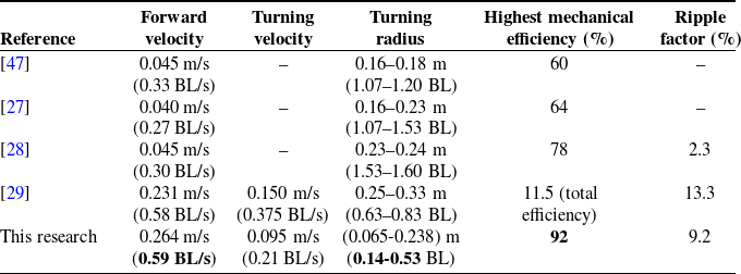
To elucidate the performance of the developed model, a comparative analysis with prior studies was conducted. According to ref. [Reference Pham, Nguyen, Lee and Vo44], the mechanical efficiency was reported to be below 10%, while ref. [Reference Pham, Nguyen, Lee and Vo29] indicated an efficiency of approximately 12%. Regarding experimental work, ref. [Reference Sfakiotakis, Fasoulas, Kavoussanos and Arapis45] reported a propulsive efficiency of around 56
 $\%$
at 1.5 Hz for an undulating fin. In contrast, ref. [Reference Behbahani and Tan28] documented a peak mechanical efficiency of 78%. The present study demonstrates a high efficiency, approaching 92%, indicating a promising improvement over existing designs under idealized conditions. However, it should be noted that this computed efficiency neglects frictional losses and the inertial effects of the oscillatory and rotational fin components.
Furthermore, to evaluate the robot’s swimming performance from a broader perspective, the Strouhal number, defined as
 $St = f_KA/v_{x,a}$
[Reference Eloy46], was examined. Here,
 $v_{x,a}$
and
 $A$
denote the mean forward velocity (see Eq. (27)) and peak-to-peak fin-tip amplitude (
 $A = 2(L_0+L)\sin \left (\gamma _{K3}^{\max }\right )$
with
 $\gamma _{K3}^{\max }$
being the amplitude of
 $\gamma _{K3}$
), respectively. The profiles of the Strouhal number for both straight and turning swimming modes are presented in Figure 25. In straight swimming, the lowest Strouhal number of 1.02, achieved at
 $n_K = 98.4$
rpm, marks the closest convergence to the optimal locomotion regime of aquatic animals (
 $0.15 \le St \le 0.8$
) [Reference Eloy46]. This correlation is highly consistent, given that the robot obtains its peak mechanical efficiency at this specific
 $n_K$
value. In contrast, for the turning mode, the Strouhal number deviates significantly from this optimal regime (
 $St \gt 1.55$
). In summary, across both swimming modes, the mechanical efficiency increases with
 $n_K$
, while the Strouhal number nearly approaches the bioinspired optimal range at elevated rotational speeds (corresponding to high-efficiency zones).
Comparison of the fish robot’s performance.

Table III. Long description
The table compares the performance metrics of different fish robots across several studies. It has six rows and six columns. The columns are labeled Reference, Forward velocity, Turning velocity, Turning radius, Highest mechanical efficiency (%), and Ripple factor (%). The row labels are [47], [27], [28], [29], and This research. Each row provides specific values for the performance metrics. For example, the first row under [47] shows a forward velocity of 0.045 meters per second, a turning velocity not specified, a turning radius of 0.16 to 0.18 meters, a highest mechanical efficiency of 60 percent, and a ripple factor not specified. The table highlights variations in performance metrics across different studies and the current research.
Simulated and experimental ripple factor
 $\gamma$
versus
 $n_K$
of the robotic fish.

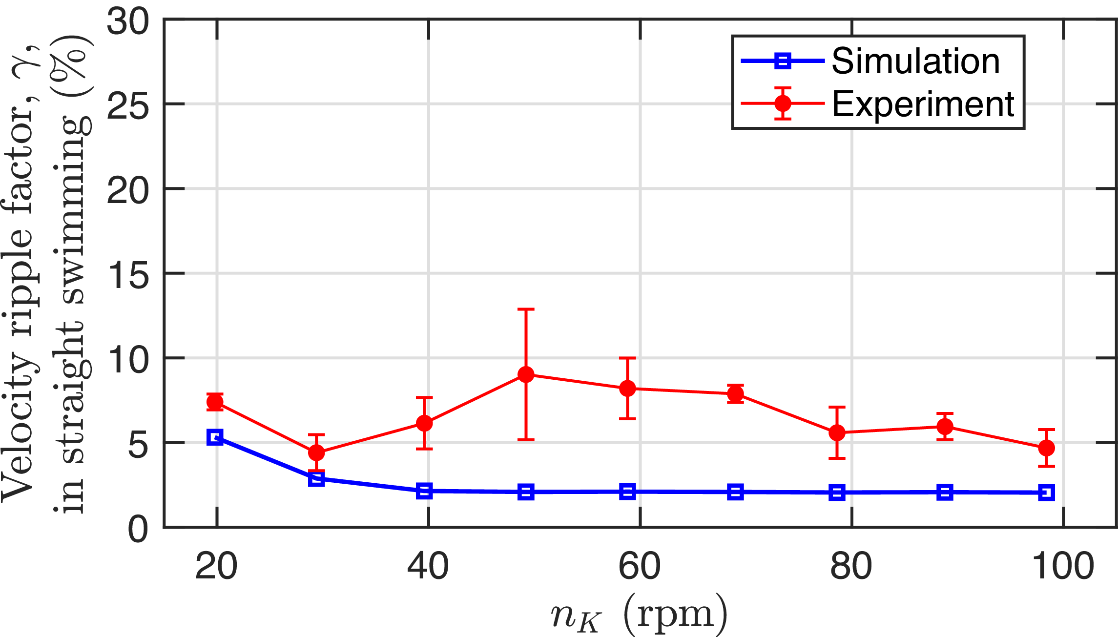
Furthermore, to evaluate the smoothness of the robot’s forward velocity – particularly for applications requiring minimal vibration – the ripple coefficient is introduced as defined in equation (26) with
 $T_S = 5\text{ s}$
. Figure 26 illustrates the relationship between this coefficient and the rotational speed
 $n_K$
at a constant phase difference angle (
 $\lvert \phi _{\gamma _{Ki}}\rvert = 61.8^\circ$
). The numerical and experimental results exhibit a satisfactory agreement, despite minor discrepancies. Specifically, the empirical ripple coefficient remains low, consistently below 9.2
 $\%$
, whereas the peak simulated value is 5.3
 $\%$
. This discrepancy is non-uniform across the range of
 $n_K$
, becoming more pronounced within the interval of 39.6 to 78.6 rpm. The maximum localized deviation reaches 6.9
 $\%$
at
 $n_K = 49.2\text{ rpm}$
. The higher values observed in the empirical data can be primarily attributed to free-surface and bounded wall effects interacting with the undulatory motion of the pectoral fins. While the numerical model assumes an infinite fluid domain, the physical experiments were conducted near the free surface with an average side-wall distance of approximately 0.68 m. Consequently, wave reflections from both the water surface and tank walls disturb the wake velocity profile, inflating the experimental fluctuations. Another contributing factor stems from the simplified unsteady hydrodynamic approximations. The core parameters,
 $C_a$
,
 $C_d$
, and
 $C_L$
within the simulation, may not perfectly capture the highly unsteady dynamic states of the physical robotic fish.
Summarily, the swimming performance of the proposed robotic fish, which incorporates pectoral fins for propulsion, was rigorously evaluated in comparison to prior designs. Table III presents a detailed comparison between the current study and several preceding publications employing similar configurations. These results underscore a moderate improvement in propulsive efficiency and overall locomotor performance for the selected fin prototype in the robotic fish design, with the mean highest forward velocity of 0.59 BL/s and a mean turning radius of 0.14–0.53 BL, albeit with a forward velocity comparable to that of an earlier study with the folding pectoral fin type observed in ref. [Reference Pham, Nguyen, Lee and Vo29]. Consistent with [Reference Pham, Nguyen, Lee and Vo29], the proposed fin design yields a slightly lower experimental ripple coefficient.
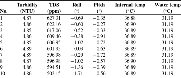
In evaluating external applications, recent approaches to water quality monitoring have focused on measuring parameters such as temperature, dissolved oxygen (DO), and pH [Reference Ji, Wei, Liu and An48], as well as water temperature, turbidity, and pH [Reference Chen, Li, Mo, Cui, Li, Lian and Gong49]. However, existing robotic fish designs primarily employ propulsion mechanisms based on caudal fins or fixed-propeller systems. To evaluate the in situ water quality monitoring capability of the proposed robotic fish, field trials were conducted in an experimental water tank. Data were sampled at 0.2 s intervals, from which ten consecutive measurements were extracted after applying a 30-point moving median filter. During the sampling period, the robot was maintained in a static-fin configuration to minimize hydrodynamic interference. The collected records encompass critical environmental parameters and the vehicle’s orientation. As summarized in Table IV, the results indicate stable turbidity levels with a mean of 4.87
 $\pm$
0.01 NTU (range: 4.85–4.89 NTU), suggesting minimal suspended particulate matter. Total dissolved solids exhibited a gradual decrease from 627.31 ppm to 502.15 ppm (mean
 $\pm$
SD: 597.55
 $\pm$
33.52 ppm), with a strong negative correlation (r = −0.76) to the sampling sequence; this trend indicates a slight data drift at the sampling location. Orientation metrics demonstrated minimal roll angles (−0.76
 $^{\circ }$
 $\pm$
0.49
 $^{\circ }$
) and pitch angles (−0.55
 $^{\circ }$
 $\pm$
0.20
 $^{\circ }$
), confirming effective stability during operation. The robot’s internal temperature was consistently maintained at 36.89
 $\pm$
0.01
 $^{\circ }$
C, while the ambient water temperature remained stable at 31.19
 $^{\circ }$
C, highlighting the reliability of thermal measurements. The accuracy of these measurements is inherently limited by sensor quality, calibration (Section 4), and data processing. This underscores the need for advanced filtering and validation techniques in future work to enhance data reliability.
6. Conclusion
The pectoral fins of robotic fish hold significant potential for locomotion. This paper presents a robotic fish design propelled by two undulating pectoral fins, each with a single DOF, enabling high maneuverability. The Morison external force model is employed to characterize the motion of the fins and the body. The robot achieves a peak forward swimming speed of
 $0.59\text{ BL/s}$
and exhibits high agility with a turning radius ranging from
 $0.14$
to
 $0.53\text{ BL}$
. Furthermore, under ideal conditions, it attains a simulated mechanical efficiency of
 $92\%$
, demonstrating its viability as a mobile platform for aquatic environmental monitoring. In the future, several key research directions are outlined as follows: (i) the development of a buoyancy control module to enable the robotic fish to adjust its depth dynamically and efficiently during locomotion; (ii) the formulation of advanced algorithms for trajectory-tracking control; (iii) further empirical validation of water quality sensors under authentic environmental settings.
Sampling results of some water environment parameters at the swimming pool.

Table IV. Long description
The table presents data from ten consecutive measurements of water quality parameters and vehicle orientation during field trials of a robotic fish in an experimental water tank. The table has ten rows and seven columns. The columns are labeled as follows: No., Turbidity (NTU), TDS (ppm), Roll (°), Pitch (°), Internal temp (°C), and Water temp (°C). The rows list the following data: Row 1: No. 1, Turbidity 4.87, TDS 627.31, Roll -0.69, Pitch -0.35, Internal temp 36.88, Water temp 31.19. Row 2: No. 2, Turbidity 4.86, TDS 622.16, Roll -0.60, Pitch -0.27, Internal temp 36.90, Water temp 31.19. Row 3: No. 3, Turbidity 4.85, TDS 617.06, Roll -0.52, Pitch -0.33, Internal temp 36.89, Water temp 31.19. Row 4: No. 4, Turbidity 4.86, TDS 609.46, Roll -0.38, Pitch -0.91, Internal temp 36.89, Water temp 31.19. Row 5: No. 5, Turbidity 4.85, TDS 606.95, Roll -1.02, Pitch -0.72, Internal temp 36.89, Water temp 31.19. Row 6: No. 6, Turbidity 4.89, TDS 601.95, Roll -0.03, Pitch -0.63, Internal temp 36.89, Water temp 31.19. Row 7: No. 7, Turbidity 4.89, TDS 596.98, Roll -0.29, Pitch -0.72, Internal temp 36.89, Water temp 31.19. Row 8: No. 8, Turbidity 4.87, TDS 596.98, Roll -1.02, Pitch -0.57, Internal temp 36.90, Water temp 31.19. Row 9: No. 9, Turbidity 4.86, TDS 594.51, Roll -1.36, Pitch -0.39, Internal temp 36.89, Water temp 31.19. Row 10: No. 10, Turbidity 4.86, TDS 502.15, Roll -1.71, Pitch -0.56, Internal temp 36.89, Water temp 31.19. The table shows stable turbidity levels, a gradual decrease in total dissolved solids, minimal roll and pitch angles, and consistent internal and water temperatures.
Acknowledgements
The authors express sincere gratitude to Pham Van Dong University for providing essential infrastructural support. This work was also supported by Ho Chi Minh City University of Technology (HCMUT) and Vietnam National University Ho Chi Minh City (VNU-HCM). The authors used Grok (xAI) and Grammarly to refine the English language and grammar during manuscript preparation. All authors have reviewed the content and take full responsibility for the final manuscript.
Author contributions
Van Anh Pham conceptualized the study, designed the research methodology, and wrote the original draft of the manuscript. Thanh Tung Tran performed the experiments and collected the data. Tuong Quan Vo contributed to the development of the design frame, reviewed, and revised the manuscript. All authors have read and approved the final version of the manuscript.
Financial support
This research received no specific grant from any funding agency, commercial or not-for-profit sectors.
Competing interests
The authors declare no conflicts of interest exist.
Ethical approval
Not applicable.
A. Appendix
 \begin{equation} \vec {i}_B = \vec {i}_W\cos \psi +\vec {j}_W\sin \psi , \end{equation}
 \begin{equation} \vec {j}_B = -\vec {i}_W\sin \psi +\vec {j}_W\cos \psi , \end{equation}
 \begin{equation} \vec {k}_B = \vec {k}_W. \end{equation}
 \begin{equation} ^Wg_{Ki} = ^Wg_B.^Bg_K.^Kg_{Ki}. \end{equation}
Where,
 \begin{equation} ^Wg_B = \begin{bmatrix} ^WR_B\;\;\;\;\; & ^Wd_B \\ O\;\;\;\;\; & 1 \end{bmatrix}\!, \end{equation}
 \begin{equation} ^Bg_K = \begin{bmatrix} ^BR_K \;\;\;\;\;& ^Bd_K \\ O\;\;\;\;\; & 1 \end{bmatrix}\!, \end{equation}
 \begin{equation} ^Kg_{Ki} = \begin{bmatrix} ^KR_{Ki}\;\;\;\;\; & ^Kd_{Ki} \\ O\;\;\;\;\; & 1 \end{bmatrix}\!, \end{equation}
 \begin{equation} {}^W R_B = \begin{bmatrix} \cos \psi\;\;\;\;\; & -\sin \psi\;\;\;\;\; & 0 \\\sin \psi\;\;\;\;\; & \cos \psi\;\;\;\;\; & 0 \\0\;\;\;\;\; & 0\;\;\;\;\; & 1 \end{bmatrix}\!, \end{equation}
 \begin{equation} {}^B R_K = \begin{bmatrix} 1\;\;\;\;\; & 0\;\;\;\;\; & 0 \\0\;\;\;\;\; & 1\;\;\;\;\; & 0 \\0\;\;\;\;\; & 0\;\;\;\;\; & 1 \end{bmatrix}\!, \end{equation}
 \begin{equation} {}^K R_{Ki} = \begin{bmatrix} 1\;\;\;\;\; & 0\;\;\;\;\; & 0 \\ 0\;\;\;\;\; & \cos \gamma _{Ki}\;\;\;\;\; & -\sin \gamma _{Ki} \\ 0\;\;\;\;\; & \sin \gamma _{Ki}\;\;\;\;\; & \cos \gamma _{Ki} \end{bmatrix}\!, \end{equation}
 \begin{equation} {}^Wd_B = \begin{bmatrix} X\;\;\;\;\; & Y\;\;\;\;\; & 0 \end{bmatrix}^T\!, \end{equation}
 \begin{equation} {}^Bd_L = \begin{bmatrix} a_1\;\;\;\;\; & b_1\;\;\;\;\; & 0 \end{bmatrix}^T\!, \end{equation}
 \begin{equation} {}^Bd_R = \begin{bmatrix} a_1\;\;\;\;\; & -b_1\;\;\;\;\; & 0 \end{bmatrix}^T\!, \end{equation}
 \begin{equation} {}^Kd_{Ki} = \begin{bmatrix} 0\;\;\;\;\; & 0\;\;\;\;\; & 0 \end{bmatrix}^T\!, \end{equation}
 \begin{equation} O = \begin{bmatrix} 0\;\;\;\;\; & 0\;\;\;\;\; & 0 \end{bmatrix}^T\!. \end{equation}
The added mass terms
 $m_x, m_y$
and the added moment of inertia
 $J_z$
are derived as follows:
 \begin{equation} \begin{cases} m_x = k_1 m_b, \\ m_y = k_2 m_b, \\ J_z = k' J_b. \end{cases} \end{equation}
The eccentricity
 $e$
is formulated as:
 \begin{equation} e = 1-\left(\frac {b_b+c_b}{2a_b}\right)^2\!. \end{equation}
The Lamb’s
 $k$
-factors
 $k_1, k_2, k'$
are functions of
 $e$
and are computed in detail within [Reference Fossen38].









 nKm
 nK=98.4


 nK=98.4


 nK
 η
 St
 γ
 nK