2·1. Recollections on maximal Cohen–Macaulay modules

For an L-graded ring R as above, or as in Sections 4 and 6, recall that graded Gorenstein means that there is an isomorphism

\begin{align*}\textrm{RHom}_{\textrm{gr}-R}(\mathbb{C},R(-\alpha))\simeq \mathbb{C}[-n],\end{align*}

where $\alpha$ is the Gorenstein parameter, n is the Krull dimension of R, and $M(l)$ for an L-graded R (or S) module is an internal grading shift such that $M(l)_i=M_{i+l}$ . The Gorenstein parameter $\alpha$ is negative (resp. zero, positive) if its projection to the $\mathbb{Z}$ -factor of L is negative (resp. zero, positive). For an invertible polynomial in two variables, this value is $-d_0$ , which is negative for all invertible polynomials in two variables other than $x^2+y^2$ , where it is zero.

Later, we will utilise Serre duality for maximal Cohen–Macaulay (MCM) modules which follows from Auslander–Reiten duality ([ Reference Auslander and ReitenAR87 ]). Recall that, when R is Gorenstein, a finitely-generated R-module is MCM if

(7) \begin{align}\textrm{Ext}_{\textrm{gr}-R}^i(M,R)=0\ \text{ for all }i\gt0,\end{align}

and the stabilised category of maximal Cohen–Macaulay modules, denoted by $\underline{\textrm{MCM}}(R)$ , has the same objects as $\textrm{MCM}(R)$ (i.e. finitely generated R modules such that (7) holds), but the morphisms are given by

\begin{align*}\underline{\textrm{Hom}}_{\textrm{gr}-R}(M,N)\;:\!=\;\textrm{Hom}_{\textrm{gr}-R}(M,N)/\mathcal{P}(M,N),\end{align*}

where $\mathcal{P}(M,N)$ are those morphisms which factor through some free R-module. For any $M,N\in \textrm{MCM}(R)$ such that $\textrm{Hom}_{\textrm{gr}-R}(M,N)$ is finite dimensional there is then Serre duality

(8) \begin{align}\underline{\textrm{Hom}}_{\textrm{gr}-R}(M,N)\simeq \underline{\textrm{Hom}}_{\textrm{gr}-R}(N,M(-\alpha)[n-1])^\vee,\end{align}

where $(-)^\vee$ is the $\mathbb{C}$ -linear dual and n is again the Krull dimension of R. Note that, in our case, the fact that $\textbf{w}$ has an isolated singularity means that all Hom-spaces are finite dimensional. For a proof of Serre duality in the $\mathbb{Z}$ -grading case, we refer to [ Reference Iyama and TakahashiIT13 , corollary 3·5], with the L-graded case we need being a straightforward generalisation.

By an L-graded matrix factorisation of rank r, $K^{\bullet}$ , we mean a two periodic sequence of L-graded, rank r, free S-modules

(9) \begin{align}K^{\bullet} = ( \cdots \rightarrow K^i \xrightarrow{k^i} K^{i+1} \xrightarrow{k^{i+1}} K^{i+2} \rightarrow \cdots ),\end{align}

where $k^{i+1}\circ k^{i}=\textbf{w} \cdot\textrm{Id}_{r}$ , and graded two-periodicity means a fixed choice of $K^{\bullet}(\vec{c})\simeq K^{\bullet}[2]$ . This presentation of a matrix factorisation naturally arises from the process of stabilisation; see, for example, [ Reference DyckerhoffDyc11 , sections 2·1 and 2·2]. Namely, one starts with a finitely generated R-module M, and considers an R-free resolution. By a famous result of Eisenbud ([ Reference EisenbudEis80 ]), any such resolution eventually becomes two periodic (i.e. stabilises). To get a matrix factorisation, we extend this two periodic complex indefinitely to the right and then replace the R modules in the complex by the corresponding free S modules. The inverse of this process is given by taking the cokernel of the map $k^0$ . In fact ([ Reference OrlovOrl09 , proposition 3·5, theorem 3·10]), there is an equivalence of categories

\begin{align*}\textrm{coker}\;:\;\textrm{HMF}(\mathbb{C}^2,\Gamma,\textbf{w})\xrightarrow{\sim}\underline{\textrm{MCM}}(R),\end{align*}

where $\textrm{HMF}(\mathbb{C}^2,\Gamma,\textbf{w})$ is the homotopy category of $\textrm{mf}(\mathbb{C}^2,\Gamma,\textbf{w})$ . Observe that, if $K^{\bullet}$ is a matrix factorisation, then we have

(10) \begin{align}K^{\bullet}[n]\mapsto \textrm{coker}((\!-\!1)^nk^n)=M[n]\end{align}

under this equivalence. We will use this fact frequently, particularly in the proofs of generation statements.

A different perspective on the category of matrix factorisations is provided by a famous result of Buchweitz and Orlov ([ Reference BuchweitzBuc86 ], [ Reference OrlovOrl09 , theorem 39]), which, generalised to stacks in [ Reference Polishchuk and VaintrobPV11 ] and applied to our setting, shows that

\begin{align*}D^b_{\textrm{sg}}([\textbf{w}^{-1}(0)/\Gamma])\simeq \textrm{HMF}(\mathbb{C}^2,\Gamma,\textbf{w}).\end{align*}

In the above, the category on the left is the derived category of singularities of the stack $[\textbf{w}^{-1}(0)/\Gamma]$ , which is defined as the quotient of the derived category of coherent sheaves on $[\textbf{w}^{-1}(0)/\Gamma]$ by the subcategory of perfect complexes. Moreover, L-graded R-modules naturally correspond to sheaves on $[\textbf{w}^{-1}(0)/\Gamma]$ , yielding an equivalence

\begin{align*}D^b_{\textrm{sg}}(\textrm{gr}-R)\simeq D^b_{\textrm{sg}}([\textbf{w}^{-1}(0)/\Gamma]).\end{align*}

Justified by the above equivalences, we will frequently switch between talking about graded R-modules, sheaves on $[\textbf{w}^{-1}(0)/\Gamma]$ and matrix factorisations. Moreover, observe that (8) and these equivalences give Serre functors on each of the categories we consider.

2·2. Graded matrix factorisations for loop polynomials

In this subsection, we introduce and study the basic objects from which we will build our tilting object. These are broadly similar to those of [ Reference Habermann and SmithHS20 , section 2·1]; however, direct computation as in loc. cit. would be intractable, since the ranks of the matrix factorisations we need to consider increases with the index of $\Gamma\subseteq \Gamma_{\textbf{w}}$ . The main technical difference is therefore the utilisation of Serre duality in order to facilitate computation. In particular, we will see that the quiver Figure 1 with $\ell=1$ corresponds on-the-nose to [ Reference Habermann and SmithHS20 , figure 1].

From the equivalences in Section 2·1, the intuition is that $\textrm{mf}(\mathbb{C}^2,\Gamma,\textbf{w})$ should correspond to structures sheaves of the irreducible components, sheaves supported at the origin (the singular point of $\textbf{w}^{-1}(0)$ ), and L-graded shifts of these. This indeed turns out to be the case.

Analogously to [ Reference Habermann and SmithHS20 ], we introduce the notation $\textbf{w}=xyw_1\ldots w_\ell$ , where

\begin{align*}w_r=x^{\frac{p-1}{\ell}}-e^{\frac{\pi\sqrt{-1}}{\ell}}\eta^ry^{\frac{q-1}{\ell}}\end{align*}

for $\eta$ a fixed primitive $\ell^{\text{th}}$ root of unity. Continuing with notation introduced in [ Reference Habermann and SmithHS20 , section 2·2], we define $w=w_1\ldots w_\ell$ . With this, there are $\ell+2$ matrix factorisations coming from ( $\Gamma$ -equivariantly) factoring $\textbf{w}$ . These correspond to

\begin{align*}{{}^{}K_{x}}^{\bullet} = ( \cdots \rightarrow S(-\vec{c}) \xrightarrow{yw} S(-\vec{x}) \xrightarrow{x} S \rightarrow \cdots ),\\ {{}^{}K_{y}}^{\bullet} = ( \cdots \rightarrow S(-\vec{c}) \xrightarrow{xw} S(-\vec{y}) \xrightarrow{y} S \rightarrow \cdots ),\end{align*}

as well as the matrix factorisations

\begin{align*}{{}^{}K_{{w_r}}}^{\bullet} = ( \cdots \rightarrow S(-\vec{c}) \xrightarrow{\textbf{w}/w_r} S(-\frac{p-1}{\ell}\vec{x}) \xrightarrow{w_r} S\rightarrow \cdots ).\end{align*}

These matrix factorisations are the obvious generalisation of the maximally graded case, and, as in that case, we also consider the objects

\begin{align*}{{}^{i}K_{x}}&={{}^{}K_{x}}((i+1-p)\vec{x})\\{{}^{j}K_{y}}&={{}^{}K_{y}}((i+1-q)\vec{y})\end{align*}

where $i=p-({p-1})/{\ell},\ldots,p-1$ and $j=q-({q-1})/{\ell},\ldots, q-1$ .

On the other hand, the generalisation of the matrix factorisations corresponding to sheaves supported at the origin require more technical considerations. Namely, for $p-({p-1})/{\ell}\leqslant i\leqslant p-1$ , $1\leqslant j\leqslant q-1$ , we set $k=\lfloor \frac{(j-1)\ell}{q-1}\rfloor$ and consider the ideal

(11) \begin{align}I_{i,j}=&\ (x^{i-(\ell-1-k)\frac{p-1}{\ell}})+\sum_{t=1}^{k}(x^{i-(\ell-k-1+t)\frac{p-1}{\ell}}y^{j-(k+1-t)\frac{q-1}{\ell}}) + (y^{j})\end{align}

(12) \begin{align}=\ (x^{i-(\ell-1-k)\frac{p-1}{\ell}}, x^{i-(\ell-k)\frac{p-1}{\ell}}y^{j-k\frac{q-1}{\ell}}, \ldots, x^{i-(\ell-1)\frac{p-1}{\ell}}y^{j-\frac{q-1}{\ell}},y^{j})\end{align}

and the L-graded R-modules

\begin{align*}R((i+1)\vec{x}+(j+1)\vec{y})/I_{i,j}.\end{align*}

The corresponding matrix factorisation, which we denote by ${{}^{i,j}K_{0}}$ , is given by stabilising this module. Namely, an R-free resolution can be built by beginning with

\begin{align*}R(\vec{c}-(k+1)\frac{p-1}{\ell}\vec{x}+j\vec{y})\oplus\bigoplus_{t=0}^{k-1}R(\vec{c})\oplus R((i+1)\vec{x}+\vec{y})\rightarrow{}R((i+1)\vec{x}+(j+1)\vec{y}),\end{align*}

where the map is multiplication by $\begin{pmatrix} {}x^{i-(\ell-1-k)({p-1})/{\ell}}& \ldots& y^{j}\end{pmatrix}$ , yielding a rank $(k+2)$ matrix factorisation. Observe in particular that substituting $\ell=1$ into this presentation recovers the definition of ${{}^{i,j}K_{0}}$ in [ Reference Habermann and SmithHS20 ]. The k terms in the middle of the ideal in (11) are all monomials of degree $i\vec{x}+j\vec{y}-(p-1)\vec{x}\ (=i\vec{x}+j\vec{y}-(q-1)\vec{y})$ .

From this, it is straightforward to check that the maps defining the matrix factorisation are given in even degree by

(13) \begin{align}\textrm{d}_0=\begin{pmatrix}y^{j-k\frac{q-1}{\ell}} & 0 & 0 & \ldots & 0 &x^{p-i+\frac{p-1}{\ell}(\ell-1-k)}y\\-x^{\frac{p-1}{\ell}}& y^{\frac{q-1}{\ell}} & 0 &\ldots& 0 & 0\\0 & -x^{\frac{p-1}{\ell}} & y^{\frac{q-1}{\ell}} & \ldots &0 & 0\\0 & 0 & -x^{\frac{p-1}{\ell}}& \ldots & 0& 0\\\vdots &\vdots & \vdots & \ddots& \vdots & \vdots \\0 & 0 & 0 & \ldots & y^{\frac{q-1}{\ell}} & 0\\0 & 0 & 0 & \ldots& -x^{i-(\ell-1)\frac{p-1}{\ell}} & xy^{q-j}\\\end{pmatrix},\end{align}

and in odd degree by $\textrm{d}_1=\textrm{Adj}(\textrm{d}_0)$ , the adjugate matrix. Explicitly, we have that ${{}^{i,j}K_{0}}$ corresponds to the matrix factorisation

where the rightmost term is in cohomological degree 0 and $\textrm{d}_0$ , $\textrm{d}_1$ map between the entire columns, not just he middle summands.

As in the maximally graded case, we are interested in a full subcategory $\mathcal{B}$ of $\textrm{mf}(\mathbb{C}^2,\Gamma,\textbf{w})$ consisting of the objects described above. Namely, let $\mathcal{B}$ be the category consisting of the $({pq-1})/{\ell}+\ell$ objects

\[\{{{}^{i,j}K_{0}}, {{}^{i}K_{x}}[3],{{}^{q-\frac{q-1}{\ell}}K_{y}}[3],\ldots, {{}^{q-1}K_{y}}[3], {{}^{}K_{w_1}}[3],\ldots, {{}^{}K_{w_\ell}}[3]\}_{i=p-\frac{p-1}{\ell}, \ldots, p-1;\ j=1, \ldots, q-1}.\]

The reason for the shifts is so that all morphisms turn out to have cohomological degree 0. In the following sections we compute the cohomology level morphisms between the objects in this category. The reader willing to take these computations on faith may skip directly to Theorem 2·8 for the characterisation of $\mathcal{B}$ as a quiver algebra.

2·3. Morphisms between the ${{}^{}K_{x}}$ ’s, ${{}^{}K_{y}}$ ’s and ${{}^{}K_{w_r}}$ ’s

As in [ Reference Habermann and SmithHS20 ], we leverage a result of Buchweitz [ Reference BuchweitzBuc86 , section 1·3, remark (a)] which establishes the following: given L-graded R-modules M and M’ with corresponding stabilisations K and K’, we have

\begin{align*}\textrm{Hom}^{\bullet}_{\textrm{HMF}(\mathbb{C}^2, \Gamma, \textbf{w})} (K, K') &\simeq \textrm{H}^{\bullet} \left(\textrm{Hom}_{\textrm{gr}-R} (K \otimes_{S} R, M')\right)\end{align*}

The Hom on the right-hand side is taken component-wise on the complex $K \otimes_S R$ . We refer to [ Reference KravetsKra19 , proposition 2·23] for a proof of the statement. Note that Buchweitz’s original remark is missing a Gorenstein assumption, and, as demonstrated in [ Reference KravetsKra19 , remark 2·24], does not hold without it.

For calculations regarding the modules ${{}^{}K_{x}}$ , ${{}^{}K_{y}}$ and ${{}^{}K_{w_r}}$ , the arguments carry over almost verbatim from the maximally graded case [ Reference Habermann and SmithHS20 , sections 2·3 and 2·4], and we have:

2·4. Morphisms between the ${{}^{}K_{w_r}}$ ’s and ${{}^{}K_{0}}$ ’s

The fact that $\textrm{Hom}^{\bullet}({{}^{}K_{w_r}}, {{}^{i,j}K_{0}})=0$ essentially follows from the arguments of [ Reference Habermann and SmithHS20 , section 2·5]. In the other direction $\textrm{Hom}^{\bullet}({{}^{i,j}K_{0}}, {{}^{}K_{w_r}})$ we argue as follows. Firstly, observe that, since $\textbf{w}$ has an isolated singularity at the origin, morphisms of R-modules are finite dimensional, and Serre duality for the corresponding MCM modules applies. We then observe that

(14) \begin{align}\dim_\mathbb{C} \textrm{Hom}^{\bullet}({{}^{}K_{w_r}},{{}^{i,j}K_{0}}(\vec{c}-\vec{x}-\vec{y}))= \begin{cases}1\qquad\text{if }\bullet=-3\\0\qquad\text{otherwise}, \end{cases} \end{align}

and so $\textrm{Hom}^{\bullet}({{}^{i,j}K_{0}}, {{}^{}K_{w_r}})$ is non-trivial only in cohomological degree three, where it is rank one; it is then straightforward to write down this non-trivial element.

Lemma 2·4. For each $r=1,\ldots,\ell$ , there is a single morphism between ${{}^{i,j}K_{0}}$ and ${{}^{}K_{w_r}}$ given by

\begin{align*} \textrm{Hom}^{3}({{}^{i,j}K_{0}},{{}^{}K_{w_r}})=\mathbb{C}\cdot\begin{pmatrix}y^{(k+1)\frac{q-1}{\ell}-j}\\e^{-\frac{\pi i}{\ell}}\eta^{-r}\\(e^{-\frac{\pi i}{\ell}}\eta^{-r})^2\\\vdots\\(e^{-\frac{\pi i}{\ell}}\eta^{-r})^{k}\\(e^{-\frac{\pi i}{\ell}}\eta^{-r})^{k+1}x^{p-1-i} \end{pmatrix}, \end{align*}

where $k=\lfloor \frac{(j-1)\ell}{q-1}\rfloor$ as before.

Proof. Observe that the complex computing the morphisms has differential given by $\textrm{d}_0^T$ in odd degree and $\textrm{d}_1^T=\textrm{Adj}(\textrm{d}_0)^T$ in even degree, where $\textrm{d}_0$ is the map from (13). It is then clear that the above vector defines an element in the kernel; the only non-trivial term to check is that it is in the kernel of the last row of $\textrm{d}_0^T$ , although this follows from observing that this factors into $(\ell-1-k)$ polynomials, one of which is $w_r$ . It is clear that this is not in the image of $\textrm{d}_1^T$ , since the $k-1$ constant elements in the kernel cannot be in the image of a degree $(({p-1})/{\ell})\vec{x}$ -map. The fact that this spans the cohomology group follows from (14).

2·5. Morphisms between ${{}^{}K_{x}}$ ’s and ${{}^{}K_{y}}$ ’s and ${{}^{}K_{0}}$ ’s

For each I we have that $\textrm{Hom}^{\bullet} ({{}^{I}K_{x}}, {{}^{i,j}K_{0}})$ vanishes, which can be computed in the same way as in the maximally graded case. In order to compute the morphisms in the other direction, we argue again by Serre duality. In particular, we have that

(15) \begin{align}\dim_\mathbb{C} \textrm{Hom}^{\bullet}({{}^{I}K_{x}},{{}^{i,j}K_{0}}(\vec{c}-\vec{x}-\vec{y}))=\begin{cases}1\qquad\text{if }I=i,\ \bullet=-3\\0\qquad\text{otherwise},\end{cases}\end{align}

and similarly there is only one morphism $\textrm{Hom}^{\bullet}({{}^{J}K_{x}},{{}^{i,j}K_{0}}(\vec{c}-\vec{x}-\vec{y}))$ in degree negative three when $J\equiv j\bmod ({q-1})/{\ell}$ , and is zero otherwise. Note that the complexes computing cohomology do not vanish identically in the cases where we claim the cohomology is zero, but the complexes are exact.

Proof. The proof follows the same strategy as the proof of Lemma 2·4. Namely, the statement about the morphisms between ${{}^{I}K_{x}}$ and ${{}^{i,j}K_{0}}$ is immediate after observing that multiplication by $y^{\bullet}$ is exact, and the only morphism from ${{}^{i,j}K_{0}}$ to ${{}^{i}K_{x}}$ is in degree three. The statement about morphisms between ${{}^{J}K_{y}}$ and ${{}^{i,j}K_{0}}$ is proved similarly, although this time multiplication by $x^{\bullet}$ is exact.

2·6. Morphisms between ${{}^{}K_{0}}$ ’s

Computing morphisms ${{}^{i,j}K_{0}}\rightarrow{{}^{I,J}K_{0}}$ is analogous to the maximally graded case. Namely, morphisms are spanned by the module

\begin{align*}\big(R/I_{I,J}\big)_{(I-i)\vec{x}+(J-j)\vec{y}}\ .\end{align*}

From this, it is immediate that there are no morphisms unless $J\geqslant j$ ; however, unlike in the maximally graded case, it is now possible to have $i\gt I$ since $(({p-1})/{\ell})\vec{x}=(({q-1})/{\ell})\vec{y}$ . Putting this together, we conclude:

Lemma 2·7. For all $i\in\{p-\frac{p-1}{\ell}, \ldots, p-1\}$ and $j\in\{1,\ldots,q-1\}$ , we have

\begin{align*}&\textrm{Hom}^{\bullet}({{}^{i,j}K_{0}}, {{}^{I,J}K_{0}})\\ &\quad\simeq\begin{cases}\text{span}_\mathbb{C}\{x^{I-i}y^{J-j}, \ldots, x^{I-i+k\frac{p-1}{\ell}}y^{(J-j)\bmod \frac{q-1}{\ell}}\}& \text{if } I\geqslant i,\ J\geqslant j\\& \text{and } \bullet=0\\\text{span}_\mathbb{C}\{x^{I-i+\frac{p-1}{\ell}}y^{J-j-\frac{q-1}{\ell}},\ldots, x^{I-i+k\frac{p-1}{\ell}}y^{(J-j)\bmod \frac{q-1}{\ell}}\}& \text{if }\ I\lt i,\\&J\geqslant j+\frac{q-1}{\ell}\\& \text{and }\bullet=0\\0&\text{otherwise.}\end{cases} &\end{align*}

2·7. The total endomorphism algebra of the basic objects

From the results of the previous sections, we see that the objects in $\mathcal{B}$ are all exceptional. In fact, the endomorphism algebra of the objects in $\mathcal{B}$ are presented as a quiver-with-relations.

Fig. 1.

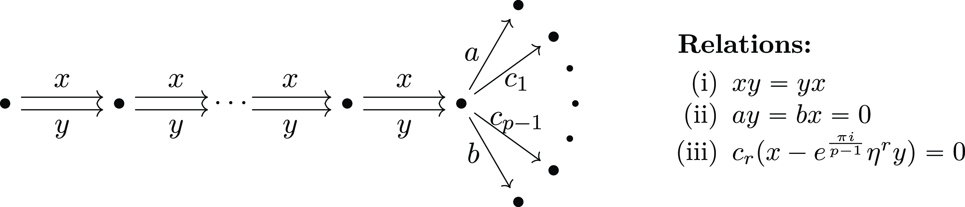
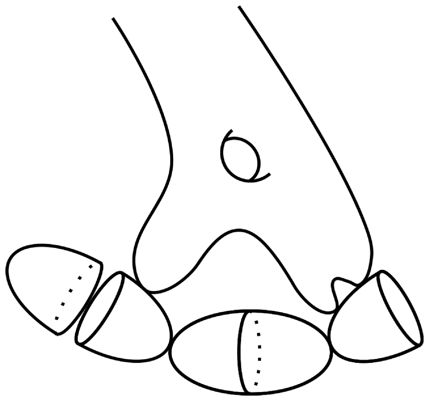
The quiver describing the category $\mathcal{B}$ for loop polynomials. There are $\ell$ blocks of size $({q-1})/{\ell}\times({p-1})/{\ell}$ .

Proof of Theorem 2·8. In order to prove the statement, all that is required is to show that the morphisms of matrix factorisations above compose in the claimed way. The first and second relations follow from the maximally graded case, [ Reference Habermann and SmithHS20 , theorem 2·13], mutatis mutandis. The third relation is not present in the maximally graded case, although checking that it holds is similarly straightforward by composing generators. Namely, consider

\begin{align*}x^{\frac{p-1}{\ell}},\ y^{\frac{q-1}{\ell}}&\in\textrm{Hom}^0({{}^{p-1,(\ell-1)\frac{q-1}{\ell}}K_{0}},{{}^{p-1,q-1}K_{0}}),\\c_r&\in\textrm{Hom}^0({{}^{p-1,q-1}K_{0}},{{}^{}K_{w_r}}[3]).\end{align*}

Following on from Remark 2·5, we compute the composition of morphisms in odd degreeFootnote ⁵ to demonstrate the relationship. In particular, the morphism $c_r$ is represented in these degrees by (a scalar multiple) of the transpose of the vector spanning the Hom-space in Lemma 2·4 after substituting $i=p-1$ , $j=q-1$ . It is a straightforward exercise to show that the morphism of matrix factorisations corresponding to $x^{\frac{p-1}{\ell}}$ is given by the $(\ell+1)\times \ell$ matrix

\begin{align*}\begin{pmatrix}1 & 0& \ldots & 0 \\0 & 1 &\ldots & 0\\\vdots &\vdots &\ddots &\vdots \\0 & 0 & \ldots & 1\\0 & 0 & \ldots & 0\end{pmatrix}\end{align*}

in odd degrees, and similarly the morphism $y^{\frac{q-1}{\ell}}$ is given in odd degrees by the matrix of the same form as above with a row of zeros in the first row and then the $\ell\times\ell$ identity matrix underneath. It is then immediate that the third relation holds.

Fig. 2.

Quiver corresponding to an alternative collection of $I_{i,j}$ for $\ell=2$ . Whilst we have considered different objects, it is clear that the resulting category is the same, since the quiver is manifestly a rearrangement of Theorem 2·8 for $\ell=2$ .

Fig. 3.

Quiver corresponding to $x^py+y^px$ .

This corresponds to a tilting module of the $\mathbb{Z}$ -graded ring $\mathbb{C}[x,y]/(x^py+y^px)$ with $|x|=|y|=1$ , and is a special case of [ Reference Buchweitz, Iyama and YamauraBIY20 , theorem 2·1].

2·8. Generation

Now that we have characterised the full subcategory $\mathcal{B}\subseteq \textrm{HMF}(\mathbb{C}^2,\Gamma,\textbf{w})$ , we aim to show that it generates. To this end, we utilise the following result of Polishchuk-Vaintrob:

It should be emphasised that Lemma 2·12 is a statement about split generation of the homotopy category $\textrm{HMF}(\mathbb{C}^2, \Gamma, \textbf{w})$ , rather than generation of the dg-category $\textrm{mf}(\mathbb{C}^2, \Gamma, \textbf{w})$ . Nevertheless, establishing that $\mathcal{B}$ split generates $\textrm{HMF}(\mathbb{C}^2, \Gamma, \textbf{w})$ is the major step towards the required generation statement.

Before giving the proof, we record the required generation result as the following corollary.

Corollary 2·14. The functor

\begin{align*} {} \textrm{Tw} \mathcal{B} \rightarrow \textrm{mf}(\mathbb{C}^2, \Gamma, \textbf{w}) {}\end{align*}

is a quasi-equivalence.

Proof. By Proposition 2·13, the functor

\begin{align*}\textrm{Tw}^\pi\mathcal{B}\rightarrow \textrm{HMF}(\mathbb{C}^2, \Gamma, \textbf{w})\end{align*}

is a quasi equivalence. Since $\mathcal{B}$ is intrinsically formal, there is also a quasi-equivalence

\begin{align*}\textrm{Tw}^\pi\mathcal{B}\rightarrow \textrm{mf}(\mathbb{C}^2, \Gamma, \textbf{w}).\end{align*}

To show that $\mathcal{B}$ generates $\textrm{mf}(\mathbb{C}^2, \Gamma, \textbf{w})$ , observe that, since $\mathcal{B}$ is a full exceptional collection in $\textrm{Tw}\mathcal{B}$ , the latter is already idempotent complete, as explained in [ Reference SeidelSei08 , remark 5·14]. Therefore, taking the idempotent completion of $\textrm{Tw}\mathcal{B}$ does nothing, and we get the result.

Proof of Proposition 2·13. We focus on the case of $\ell\gt 1$ in order to differentiate it from [ Reference Habermann and SmithHS20 , proposition 2·14], only explaining the modifications needed to incorporate the change of grading. Namely, let

\begin{align*} {}V=\{{{}^{i}K_{x}},{{}^{j}K_{y}},{{}^{}K_{w_r}},{{}^{i,j}K_{0}}\} {}\end{align*}

be the objects of $\mathcal{B}$ . We then show that $R(l)/(x,y)\in\langle V\rangle$ for any $l\in L$ and appeal to Lemma 2·12 to show that V split-generates $\textrm{HMF}(\mathbb{C}^2,\Gamma,\textbf{w})$ .

Since [2] is equivalent to $(\vec{c})$ , we must only show that $R(l)/(x,y)\in\langle V\rangle$ for $l\in L/\mathbb{Z}\vec{c}\simeq\mathbb{Z}/\left(\frac{pq-1}{\ell}\right)$ . The argument to build the modules

\begin{gather*}\{R(a\vec{x}+b\vec{y})/(x,y)\}_{\{p-\frac{p-1}{\ell}+1\leqslant a\leqslant p,\ 2\leqslant b\leqslant q\}}\\\{R(a\vec{x}+\vec{y})/(x,y)\}_{\{p-\frac{p-1}{\ell}\leqslant a\leqslant p-1\}}\\\{R((p-\frac{p-1}{\ell})\vec{x}+b\vec{y})/(x,y)\}_{\{1\leqslant b\leqslant \frac{q-1}{\ell}+1\}}\end{gather*}

with the exception of $R((p-({p-1})/{\ell})\vec{x}+\vec{y})/(x,y)$ in the second collection of modules and $R(\vec{c})/(x,y)$ in the third carry over from [ Reference Habermann and SmithHS20 , proposition 2·14] essentially unchanged. Note that, along the way, we built the modules

(16) \begin{align} \begin{split} R(a\vec{x})/(x), & \qquad\text{for } 1\leqslant a\leqslant p-1 \\ R(b\vec{y})/(y) & \qquad\text{for } 1\leqslant b\leqslant q-1, \end{split} \end{align}

and we will repeatedly appeal to this fact.

To build $R((p-({p-1})/{\ell})\vec{x}+\vec{y})/(x,y)$ , we begin by constructing ${{}^{}K_{w_r}}(l\vec{x})$ for $l=0,\ldots, (\ell-1)({p-1})/{\ell}$ and any $r=1,\ldots,\ell$ . Firstly, we have that

\begin{align*}R(\vec{x})/(w_r)\simeq\textrm{Cone}\Big(R((1-\frac{p-1}{\ell})\vec{x})/(x)\xrightarrow{w_r}R(\vec{x})/(xw_r)\Big).\end{align*}

The domain of this morphism is ${{}^{p-\frac{p-1}{\ell}}K_{x}}$ , whilst the codomain can be constructed as an extension of $R(\vec{x})/(x)$ by $R/(w_r)$ . From this, we build $R(2\vec{x})/(xw_r)$ as the extension

\begin{align*}0\rightarrow R(\vec{x})/(w_r)\xrightarrow{x}R(2\vec{x})/(xw_r))\rightarrow R(2\vec{x})/(x)\rightarrow 0,\end{align*}

where the module $R(2\vec{x})/(x)$ was constructed in (16). From this, we get

\begin{align*}R(2\vec{x})/(w_r)\simeq\textrm{Cone}\big(R((2-\frac{p-1}{\ell})\vec{x})/(x)\xrightarrow{w_r}R(2\vec{x})/(xw_r)\big),\end{align*}

where the domain is in (16), and the codomain was constructed immediately above. We then proceed inductively, alternatingly constructing $R(l\vec{x})/(xw_r)$ and then ${{}^{}K_{w_r}}(l\vec{x})$ for $l=0,\ldots, (\ell-1)({p-1})/{\ell}$ (appealing to (16) once $l\gt({p-1})/{\ell}$ . Note that this argument is valid for any $r=1,\ldots, \ell$ .

With these modules constructed, we then iteratively construct the following modules.

\begin{gather*}0\rightarrow R/(w_1)\xrightarrow{w_2}R(\frac{p-1}{\ell}\vec{x})/(w_1w_2)\rightarrow R(\frac{p-1}{\ell}\vec{x})/(w_2)\rightarrow 0\\0\rightarrow R(\frac{p-1}{\ell}\vec{x})/(w_1w_2)\xrightarrow{w_3}R(2\frac{p-1}{\ell}\vec{x})/(w_1w_2w_3)\rightarrow R(2\frac{p-1}{\ell}\vec{x})/(w_3)\rightarrow 0\\\vdots\\\begin{aligned}0\rightarrow R((\ell-1)\frac{p-1}{\ell}\vec{x})/(w_1w_2\ldots w_{\ell-1})\xrightarrow{w_{\ell}}R&((\ell-1)\frac{p-1}{\ell}\vec{x})/(w_1w_2w_3\ldots w_{\ell})\\&\rightarrow R(((\ell-1)\frac{p-1}{\ell})\vec{x})/(w_{\ell})\rightarrow 0\end{aligned}\end{gather*}

We then observe that $R((\ell-1)(({p-1})/{\ell})\vec{x})/(w_1w_2w_3\ldots w_{\ell})[1]=R((p-({p-1})/{\ell})\vec{x}+\vec{y})/(xy)$ (cf. (10)), and so we can construct $R((p-({p-1})/{\ell})\vec{x}+\vec{y})/(x,y)$ as the cone of the morphism

\begin{align*} R((\ell-1)\frac{p-1}{\ell})\vec{x}+\vec{y})/(y)& \\\bigoplus \xrightarrow{\ \ \ \ (x\ y)\ \ \ \ } & R((p-\frac{p-1}{\ell})\vec{x}+\vec{y})/(xy).\\ R((p-\frac{p-1}{\ell})\vec{x})/(x)&\end{align*}

Note that $R((\ell-1)({p-1})/{\ell})\vec{x}+\vec{y})/(y)=R(q-(({q-1})/{\ell})y)/(y)$ , and so both modules in the domain are in (16).

Finally, all that is left to do is construct the module $R(\vec{c})/(x,y)$ , which we again do iteratively.

\begin{gather*}0\rightarrow R(\vec{c}-(\frac{q-1}{\ell}+1)\vec{y})/(x)\xrightarrow{y} R(\vec{c}-\frac{q-1}{\ell}\vec{y})/(x)\rightarrow R(\vec{c}-\frac{q-1}{\ell}\vec{y})/(x,y)\rightarrow 0\\0\rightarrow R(\vec{c}-\frac{q-1}{\ell}\vec{y})/(x)\xrightarrow{y} R(\vec{c}-(\frac{q-1}{\ell}-1)\vec{y})/(x)\rightarrow R(\vec{c}-(\frac{q-1}{\ell}-1)\vec{y})/(x,y)\rightarrow 0\\\vdots\\0\rightarrow R(\vec{c}-2\vec{y})/(x)\xrightarrow{y} R(\vec{c}-\vec{y})/(x)\rightarrow R(\vec{c}-\vec{y})/(x,y)\rightarrow 0.\end{gather*}

The module $R(\vec{c}-(({q-1})/{\ell}+1)\vec{y})/(x)=R((\ell-1)({p-1})/{\ell}\vec{x})/(x)$ is from (16), and the modules on the right of the above short exact sequences are graded stabilisations of the origin which have been previously constructed. Putting this all together, we have

\begin{align*}R(\vec{c})/(x,y)\simeq\textrm{Cone}(R(\vec{c}-\vec{y})/(x)\xrightarrow{y}& R(\vec{c})/(x))\end{align*}

where the term on the domain was constructed above and the codomain is ${{}^{p-1}K_{x}}[2]$ .

We deduce the following corollary, whose proof follows from Corollary 2·14 and Theorem in the same way as in the proof of [ Reference Habermann and SmithHS20 , theorem 2·19]:

Corollary 2·15 (Corollary 1, undeformed loop polynomial case). The object

\begin{align*}\mathcal{E}\;:\!=\;\left(\bigoplus_{\substack{i=p-\frac{p-1}{\ell},\ldots, p-1\\ {} {}j=1,\ldots, q-1}}{{}^{i,j}K_{0}}\right)\oplus&\left(\bigoplus_{\substack{i=p-\frac{p-1}{\ell},\ldots, p-1}}{{}^{i}K_{x}}[3]\right)\\ {}\oplus {}&\left(\bigoplus_{\substack{j=q-\frac{q-1}{\ell},\ldots, q-1}}{{}^{j}K_{y}}[3]\right)\oplus\left(\bigoplus_{\substack{r=1,\ldots, \ell}}{{}^{}K_{w_r}}[3]\right)\end{align*}

is a tilting object for $\textrm{mf}(\mathbb{C}^2,\Gamma,\textbf{w})$ .

3·1. The crepant resolution of the $A_{\ell-1}$ singularity

We begin this section with a recounting of the classically understood crepantFootnote ⁶ resolution of du Val singularities of type A – see, for example [ Reference ReidRei03 ]. This subsection will be applicable to all invertible polynomials in two variables.

Recall that the $A_{\ell-1}$ singularity is defined as $\mathbb{C}^2/\mu_{\ell}=X=\textrm{Spec}\mathbb{C}[x,y]^{\mu_\ell}\simeq\textrm{Spec}\mathbb{C}[u,v,w]/(uv-w^{\ell})$ , where $\mu_\ell$ acts by $\xi\cdot(\check{x},\check{y})=(\xi \check{x},\xi^{-1}\check{y})$ . The crepant resolution is

\begin{align*}\pi\;:\;\widetilde{X}\rightarrow X,\end{align*}

where

\begin{align*}\widetilde{X}=\bigcup_{i=1}^{\ell}\widetilde{X}_i,\end{align*}

and each $\widetilde{X}_i\simeq \mathbb{C}^2_{(\lambda_i,\mu_i)}$ . Here, the coordinates $\lambda_i,\mu_i$ are related to the coordinates on X by $\lambda_i=u/w^{i-1}$ , $\mu_i=w^i/u$ where this makes sense. Correspondingly, the transition functions are given by

\begin{align*}\widetilde{X}_i\setminus(\mu_i=0)&\xrightarrow{\sim} \widetilde{X}_{i+1}\setminus(\lambda_{i+1}=0)\\(\lambda_i,\mu_i)&\mapsto (\mu_i^{-1},\mu_i^2\lambda_i).\end{align*}

On each chart, the resolution is given as

\begin{align*}\pi|_{\widetilde{X}_i}\;:\;\mathbb{C}^2_{(\lambda_i,\mu_i)}&\rightarrow X\\(\lambda_i,\mu_i)&\mapsto (\lambda_i^i\mu_i^{i-1},\lambda_i^{\ell-i}\mu_i^{\ell+1-i},\lambda_i\mu_i).\end{align*}

This resolution is constructed by iterated blowups of X. An important fact is that the blowup process yields an embedding of $\widetilde{X}$ into $\mathbb{C}^3\times\mathbb{P}^2\times\ldots\times\mathbb{P}^2$ , where there are ${\lfloor{\ell}/{2}\rfloor}$ factors of $\mathbb{P}^2$ . We define the symplectic form $\omega_{\widetilde{X}}$ to be the pullback of the product of the standard symplectic form on $\mathbb{C}^3$ and the Fubini–Study form on the $\mathbb{P}^2$ factors. We also drop $\widetilde{X}$ from the notation and refer to the symplectic form simply as $\omega$ , since we believe that no confusion can arise. This form is simple to write down in a given patch, although has quite a few terms. As an example, in the patch $\widetilde{X}_1$ , it is given by

\begin{align*}\phi^*_1\omega&= \frac{i}{2}\Big((1+|\mu_1|^2+|\mu_1|^4)\textrm{d}\lambda_1\wedge\textrm{d}\bar{\lambda}_1+(\lambda_1\bar{\mu}_1+2|\mu_1|^2\lambda_1\bar{\mu}_1)\textrm{d}\mu_1\wedge\textrm{d}\bar{\lambda}_1\\[5pt]&\quad+(\mu_1\bar{\lambda}_1+2|\mu_1|^2\mu_1\bar{\lambda}_1)\textrm{d}\lambda_1\wedge\textrm{d}\bar{\mu}_1+(4|\lambda_1|^2|\mu_1|^2+|\lambda_1|^2)\textrm{d}\mu_1\wedge\textrm{d}\bar{\mu}_1\\[5pt]&\quad+\frac{(1+4|\mu_1|^2+|\mu_1|^4)\textrm{d}\mu_1\wedge\textrm{d}\bar{\mu}_1}{(1+|\mu_1|^2+|\mu_1|^4)^2}\Big),\end{align*}

where $\phi_1\;:\;\widetilde{X}_1\rightarrow \widetilde{X}$ is the inclusion of the chart $\widetilde{X}_1\simeq \mathbb{C}^2_{(\lambda_1,\mu_1)}$ . It is extremely important that, since the spheres in the exceptional locus are holomorphic, $\omega$ is not exact.

In terms of writing down $[\omega]\in H^2(\widetilde{X})$ , observe that in the case $\ell=2$ , then $\widetilde{X}=\textrm{tot}\ \mathcal{O}_{\mathbb{P}^1}(-2)=T^*\mathbb{P}^1$ , and $[\omega]=2[\pi^*\omega_{\textrm{FS}}]=-\pi[\textrm{PD}(C)]$ , where C is the exceptional sphere, and $\omega_{\textrm{FS}}$ is the Fubini–Study form on $\mathbb{P}^1$ (see, for example, [ Reference RitterRit14 ]). Symplectically, the crepant resolution of the $A_{\ell-1}$ is the completion of $\ell-1$ copies of $\mathbb{D}T^*\mathbb{P}^1$ plumbed together according to the $A_{\ell-1}$ Dynkin diagram, where the symplectic form on each factor is as above. Therefore, each exceptional sphere has symplectic area $2\pi$ . Putting this all together, the symplectic form we work with on the total space has cohomology class

(17) \begin{align}[\omega]=-\pi\frac{\ell^2}{4}\textrm{PD}(C_{\frac{\ell}{2}})-\sum_{r=1}^{\frac{\ell}{2}-1}r\pi(\ell-r)(\textrm{PD}(C_r)+\textrm{PD}(C_{\ell-r}))\end{align}

for $\ell$ even, and

(18) \begin{align}[\omega]=-\sum_{r=1}^{\frac{\ell-1}{2}}r\pi(\ell-r)(\textrm{PD}(C_r)+\textrm{PD}(C_{\ell-r}))\end{align}

for $\ell$ odd, where $C_r$ are the exceptional spheres. It goes back to work of Brieskorn, [ Reference BrieskornBri66 ], that the Milnor fibre and minimal resolution of an ADE singularity are diffeomorphic (in fact, work of Ohta–Ono, [ Reference Ohta and OnoOO05 ], show that there is a unique diffeomorphism type for symplectic fillings of the link of a simple singularity). On the other hand, they are very different as symplectic manifolds – the standard symplectic form on the Milnor fibre is exact. In this work, we insist on equipping the total space $\widetilde{X}$ with the symplectic structure as above.

3·2. Equivariant Morsifications

In the introduction, we stated that we are associating a Fukaya–Seidel category to a specific equivariant Morsification of the superpotential. In this subsection, we justify this definition.

The Fukaya–Seidel category for a hypersurface singularity, as defined in [ Reference SeidelSei08 ], is independent of all choices, up to derived equivalence. In particular, it is independent of the choice of Morsification. We would like to be able to make the same statement about equivariant Morsifications; however, it quickly becomes clear that, whilst Morsifications abound, equivariant Morsifications are quite special. In particular, it is easy to cook up examples of superpotentials which have no equivariant Morsifications. The following seems to be the simplest such example.

Example 3·1. Let $\check{\textbf{w}}=x^4+y^4\;:\;\mathbb{C}^2\rightarrow \mathbb{C}$ and $G=\langle \alpha,\beta|\ \alpha^2=\beta^2=(\alpha\beta)^2=-1\rangle\subseteq\textrm{SL}(2,\mathbb{C})$ . Concretely G, acts on $\mathbb{C}^2$ via

\begin{align*} {}\alpha=\begin{pmatrix} {}\varepsilon & 0 \\ {}0 & \varepsilon^{-1} {}\end{pmatrix},\ \beta=\begin{pmatrix} {}0 & 1 \\ {}-1 & 0 {}\end{pmatrix}, {}\end{align*}

where $\varepsilon$ is a fixed 4th root of unity. The invariant polynomials are $u=x^5y-xy^5$ , $v=x^4+y^4$ and $w=x^2y^2$ , and adding any combination of u,v or w does not yield a polynomial with only non-degenerate critical points. Therefore, $\check{\textbf{w}}$ cannot be equivariantly Morsified.

On the other hand, if equivariant Morsifications exist, it seems reasonable to expect in general that the resulting category is independent of this choice by a deformation-invariance argument, as in the non-equivariant case. We avoid questions of this nature in general, and instead demonstrate this only in the case at hand.

Restricting to the case of $\ell\gt 1$ , so that we are not in the maximally graded case, one must add monomials in the Jacobian which are divided by $x^{\ell}$ , $y^{\ell}$ or xy in order to equivariantly Morsify $\check{\textbf{w}}$ . For $\ell\gt2$ , it is immediate that adding any linear combination of $x^{\ell}$ and $y^{\ell}$ or powers thereof does not Morsify the polynomial – the critical point at the origin remains degenerate. On the other hand, the origin is a non-degenerate critical point for any deformation of $\check{\textbf{w}}$ where we add any linear combination of $x^{\ell}$ , $y^{\ell}$ , xy or higher powers, provided the coefficient of xy is non-trivial. In particular, any equivariant Morsification of $\check{\textbf{w}}$ is a further deformation of the resonant Morsification $\check{\textbf{w}}_{\varepsilon}$ . For $\ell=2$ , one can now also equivariantly Morsify by adding $\varepsilon_1x^2+\varepsilon_2y^2$ for $\varepsilon_i\neq0$ , although this can similarly be deformed through polynomials with non-degenerate critical points to the resonant Morsification. Therefore, the space of equivariant Morsifications is path-connected, and the resulting categories will be derived equivalent by a deformation invariance argument, as in the non-equivariant case. We therefore feel justified in defining $\mathcal{FS}(\check{\widetilde{\textbf{w}}}_\varepsilon)$ to be the Fukaya–Seidel category associated $\check{\widetilde{\textbf{w}}}$ .

The second subtle point of defining the orbifold Fukaya–Seidel category of an equivariant Morsification is the order of pulling back and deforming the polynomial. In this paper, we will insist on equivariantly Morsifying and then pulling back. The reason is that, if one were to pull back $\check{\overline{\textbf{w}}}$ (without Morsifying), then the exceptional locus would be critical. It therefore doesn’t seem to make sense to ‘Morsify’, since this would imply that this critical locus splits into a Milnor number’s worth of critical points. Even if one were to ignore this and deform the superpotential, only requiring that it becomes non-degenerate on each chart and that this patches together to something globally defined, this is equivalent to pulling back a superpotential on X which comes from an equivariant Morsification.

3·3. Definition of the Fukaya–Seidel category for a non-exact total space

Whilst the A–model strategy follows that of [ Reference Habermann and SmithHS20 ], there are technical subtleties in this setting due to the non-exactness. In particular, the exactness of the total space is key in the construction of the Fukaya–Seidel category in [ Reference SeidelSei08 ] by ruling out sphere and disc bubbling. Since our total space is non-exact, we follow the strategy of [ Reference Auroux, Katzarkov and OrlovAKO08 , section 3], who also allow for non-exact total spaces and Lagrangians by demanding the following two conditions:

1. (i) the smooth fibre $\Sigma$ is exact;

2. (ii) the homotopy group $\pi_2(\Sigma)$ and the relative homotopy group $\pi_2(\Sigma,V_i)$ , for any (potentially non-exact) vanishing cycle $V_i$ , vanish.

These conditions are both fulfilled in our case. The first requirement follows from the fact that the fibre is a punctured surface, and so every two-form is exact. The vanishing of $\pi_2(\Sigma)$ follows from the uniformisation theorem for Riemann surfaces, whilst nontrivial $\pi_2(\Sigma,V_i)$ implies that $V_i$ is trivial in homology. In our construction, we only consider Lagrangians which are nontrivial in homology.

Another subtlety about working with a non-exact total space is that we must work over the Novikov field, defined as

\begin{align*}\Lambda_\mathbb{C}\;:\!=\;\left\{\sum_{i\geqslant 1}a_iT^{\lambda_i}|\ a_i\in\mathbb{C},\ \lambda_i\in\mathbb{R},\ \lim_{i\rightarrow \infty}\lambda_i\rightarrow\infty \right\}.\end{align*}

In general, this is crucial for two reasons. The first is that there can be infinitely many discs contributing to a given $A_\infty$ operation, and the sum is not guaranteed to converge. As a consequence of Gromov compactness, the sum converges in the Novikov field. Fortunately, we will see that this is not an issue for us, since the only non-trivial operation is the product, and there are only finitely many discs contributing to this.

The second crucial consequence of working over the Novikov field is Hamiltonian invariance. Even when sums converge, it is possible to lose Hamiltonian invariance when specialising the Novikov parameter. The essential point is that $T^A=T^B$ if and only if $A=B$ , but the multivalued-ness of the complex logarithm means that $z^A=z^B$ does not imply $A=B$ for any $z\in\mathbb{C}$ unless one were to restrict the values of A and B so as not to cross the branch locus. This is what we do, only checking that Hamiltonian invariance is preserved between Lagrangians which we are allowing as objects in our category, rather than any possible Lagrangian.

Another technical point which can’t be handled as in the maximally graded case is that, in order for the construction of the Fukaya–Seidel category to be well-defined, we need there to be a complete Kähler metric on the total space, with respect to which the gradient flow of $\check{\widetilde{\textbf{w}}}$ is bounded from below outside of a compact set. In the maximally graded setting, this follows from the polynomials being tame in the sense of [ Reference BroughtonBro88 , proposition 3·11], however, this no longer applies directly, since the total space in the case at hand is not $\mathbb{C}^n$ . Nevertheless, we can appeal to the tameness of invertible polynomials to demonstrate that $|\nabla\check{\widetilde{\textbf{w}}}|$ is bounded from below outside of a compact set.

Observe that, by construction, we have an isomorphism $(\mathbb{C}^2\setminus{\mathbb{D}^2})/\check{\overline{\Gamma}}\simeq \widetilde{X}\setminus{U}$ , where $\mathbb{D}^2$ is a small disc centred at the origin in $\mathbb{C}^2$ , and U is a tubular neighbourhood of the exceptional locus in $\widetilde{X}$ . Since $\check{\textbf{w}}\;:\;\mathbb{C}^2\rightarrow \mathbb{C}$ is tame, it remains so when it descends to $(\mathbb{C}^2\setminus{\mathbb{D}^2})/\check{\overline{\Gamma}}$ since the action of $\check{\overline{\Gamma}}$ is free away from the origin. By the above isomorphism, this shows that $|\nabla\check{\widetilde{\textbf{w}}}|$ is bounded from below on $\widetilde{X}\setminus U$ with respect to the metric induced from the blow-up construction (which agrees with the metric on $(\mathbb{C}^2\setminus{\mathbb{D}^2})/\check{\overline{\Gamma}}$ away from the exceptional locus).

To summarise, we have that $\check{\widetilde{\textbf{w}}}_\varepsilon\;:\;\widetilde{X}\rightarrow \mathbb{C}$ defines a Lefschetz fibration. We take $\mathcal{A}_{\check{\overline{\Gamma}}}$ to be a collection of Lagrangian branes in the smooth fibre (which is well-defined by the preceding paragraph), and check that Hamiltonian invariance is preserved between these branes for a given choice of Novikov parameter specialisation. We then define, as in [ Reference Auroux, Katzarkov and OrlovAKO08 ], the Fukaya–Seidel category (over $\mathbb{C}$ ) as $ \mathcal{FS}(\check{\widetilde{\textbf{w}}})\;:\!=\;\textrm{Tw} \mathcal{A}_{\check{\overline{\Gamma}}}$ .

3·4. A resonant Morsification

In the maximally graded case studied in [ Reference Habermann and SmithHS20 , section 3], a Morsification $\check{\textbf{w}}_\varepsilon=\check{x}^p\check{y}+\check{y}^q\check{x}-\varepsilon \check{x}\check{y}$ with particularly nice properties was used. Such a Morsification was called resonant, and allowed the symmetry present to be maintained and ultimately exploited. Whilst it was not considered in the maximally graded setting, the resonant Morsifications are in fact also equivariant for any $\check{\overline{\Gamma}}\simeq\mu_\ell$ . Therefore, such a Morsification descends to a map $\check{\overline{\textbf{w}}}_\varepsilon\;:\;X\rightarrow \mathbb{C}$ given by

\begin{align*}\check{\overline{\textbf{w}}}_\varepsilon(u,v,w)=w(u^{\frac{p-1}{\ell}}+v^{\frac{q-1}{\ell}}-\varepsilon).\end{align*}

Pulling this back to the chart $\widetilde{X}_i\simeq\mathbb{C}^2_{(\lambda_i,\mu_i)}$ of the crepant resolution $\widetilde{X}$ yields

\begin{align*}\check{\widetilde{\textbf{w}}}_{i,\varepsilon}(\lambda_i,\mu_i)=\lambda_i\mu_i(\lambda_i^{\frac{i(p-1)}{\ell}}\mu_i^{\frac{(i-1)(p-1)}{\ell}}+\lambda_i^{\frac{(\ell-i)(q-1)}{\ell}}\mu_i^{\frac{(\ell+1-i)(q-1)}{\ell}}-\varepsilon)\end{align*}

and this patches together to give a globally defined map $\check{\widetilde{\textbf{w}}}_{\varepsilon}\;:\;\widetilde{X}\rightarrow \mathbb{C}$ . From now on, we will refer to the restrictions of $\check{\widetilde{\textbf{w}}}_\varepsilon$ to the charts as $\check{\widetilde{\textbf{w}}}_{i}$ , with the reference to $\varepsilon$ left implicit.

Analogously to the maximally graded case, the critical points of $\check{\widetilde{\textbf{w}}}_\varepsilon$ can be grouped into four types:

1. (i) $\mu_1=0$ , $\lambda_1^{\frac{p-1}{\ell}}=\varepsilon$ ;

2. (ii) $\mu_\ell^{\frac{q-1}{\ell}}=\varepsilon$ , $\lambda_\ell=0$ ;

3. (iii) $\mu_i=\lambda_i=0$ for $i=1,\ldots, \ell$ ;

4. (iv) $\lambda_1^{\frac{p-1}{\ell}}=\frac{q-1}{pq-1}\varepsilon$ , $\lambda_1^{\frac{(\ell-1)(q-1)}{\ell}}\mu_1^{q-1}=\frac{p-1}{pq-1}\varepsilon$ .

Note that the critical points of type (iv) can equivalently be described in any of the charts of $\widetilde{X}$ ; we have given them in the first for convenience. The critical points in the first three groups have critical value 0, whilst those in the last have critical value

\begin{align*}\frac{-\varepsilon\mu_1\lambda_1}{pq-1}.\end{align*}

As in our previous work, there is a clear symmetry of these critical points. Namely, let $(\lambda_{1,\text{crit}}^+,\mu_{1,\text{crit}}^+)$ be the unique positive real critical point of type (iv) in the chart $\widetilde{X}_1$ , with corresponding critical value $c_{\text{crit}}$ . Letting $\zeta$ and $\eta$ denote the roots of unity

(19) \begin{align}\zeta = e^{2\pi i/(p-1)} \quad \text{and} \quad \eta = e^{2\pi i/(q-1)},\end{align}

we see that there is a $\mu_{p-1}\times\mu_{q-1}$ action on the critical points of type (iv) given by

\begin{align*}\{(\zeta^{m\ell}\lambda_{1,\text{crit}}^+, \zeta^{m(1-\ell)}\eta^n\mu_{1,\text{crit}}^+) \;:\; 0 \leqslant m \leqslant p-2\text{, } 0 \leqslant n \leqslant q-2\}.\end{align*}

The critical value corresponding to $(\zeta^{m\ell}\lambda_{1,\text{crit}}^+, \zeta^{m(1-\ell)}\eta^n\mu_{1,\text{crit}}^+))$ is $\zeta^m\eta^nc_{\textrm{crit}}$ , so there are $\frac{\gcd(p-1, q-1)}{\ell}$ critical points in each of these critical fibres. In order to describe each critical point of type (iv) uniquely with respect to the symmetry and the reference critical point, we restrict to the subset

(20) \begin{align}\{(\zeta^{m\ell}\lambda_{1,\text{crit}}^+, \zeta^{m(1-\ell)}\eta^n\mu_{1,\text{crit}}^+) \;:\; 0 \leqslant m \leqslant \frac{p-1}{\ell}-1\text{, } 0 \leqslant n \leqslant q-2\}.\end{align}

We do not require this to be a subgroup or have any other additional structure – all we require is that this is a collection of elements in $\mu_{p-1}\times\mu_{q-1}$ such that each point in this collection corresponds to a critical point of type (iv).

Our strategy for understanding the Fukaya–Seidel category of $\check{\widetilde{\textbf{w}}}_\varepsilon$ is essentially modelled on the strategy of the maximally graded case. Namely, we fix our regular fibre $\Sigma$ to be $\check{\widetilde{\textbf{w}}}^{-1}_1(\!-\delta)$ where $\delta$ is a positive real number much less than $\varepsilon$ (in other words, we take $*=-\delta$ ). This reference fibre is equivalently described in any of the charts, and is equivalent to the quotient of the Milnor fibre of $\check{\textbf{w}}$ by $\check{\overline{\Gamma}}$ , as studied in [ Reference HabermannHab21 , section 6·1]. For the critical points of types (i)–(iii) we follow the strategy employed in the maximally graded case and define the vanishing path given by the straight line segment from $-\delta$ to 0. For the critical point $(\zeta^{m\ell}\lambda_{1,\text{crit}}^+, \zeta^{m(1-\ell)}\eta^n\mu_{1,\text{crit}}^+)$ , meanwhile, we define the preliminary vanishing path $\gamma_{m,n}$ by following the circular arc $-\delta e^{i\theta}$ as $\theta$ increases from 0 to

\begin{align*}\theta_{m,n} \;:\!=\; 2\pi \left(\frac{m}{p-1}+\frac{n}{q-1}\right)\end{align*}

and then following the radial straight line segment from $-\zeta^m\eta^n\delta$ to $\zeta^m\eta^nc_{\textrm{crit}}$ . The preliminary vanishing paths are then altered to the temporary, and then final, vanishing paths in the same way as the maximally graded case.

3·5. The zero-fibre and its smoothing

The fibre of $\check{\widetilde{\textbf{w}}}_\varepsilon$ over zero has $\ell+2$ components: in the charts $\widetilde{X}_1$ and $\widetilde{X}_\ell$ , there are the line $\{\mu_1=0\}$ and $\{\lambda_\ell=0\}$ , respectively. The complex lines $(0,\mu_i)$ and $(\lambda_{i+1},0)$ patch together to give $\ell-1$ projective lines in an $A_{\ell-1}$ configuration. Finally, there is the curve given in local charts by $\check{w}_i=\check{\widetilde{\textbf{w}}}_i\lambda_i^{-1}\mu_i^{-1}$ . This fibre is sketched in Figure 4.

Fig. 4.

Sketch of the fibre of $\check{\widetilde{\textbf{w}}}_\varepsilon$ above the origin. This does not represent any specific polynomial, and is only meant to convey the general shape. See Figure 7 for a specific example.

Upon smoothing to $\check{\widetilde{\textbf{w}}}_\varepsilon^{-1}(\!-\delta)$ , each of the nodes is smoothed to a thin neck whose waist curve is the corresponding vanishing cycle in $\Sigma$ . We denote these vanishing cycles by ${{}^{m}V_{\mu_1\check{w}_1}}$ , ${{}^{n}V_{\lambda_\ell\check{w}_\ell}}$ and ${{}^{}V_{\mu_i\lambda_i}}$ for $m=0, \ldots, ({p-1})/{\ell}-1$ , $n=0, \ldots, ({q-1})/{\ell}-1$ and $i=1,\ldots,\ell$ , corresponding to critical pointsFootnote ⁷ $(\zeta^{m\ell}\sqrt[\frac{p-1}{\ell}]{\varepsilon}, 0)$ , $(0, \eta^{n\ell}\sqrt[\frac{q-1}{\ell}]{\varepsilon})$ and $(\lambda_i,\mu_i)=(0, 0)$ respectivelyFootnote ⁸ .

Remark 3·3. The topology of the smooth fibre was computed in [ Reference HabermannHab21 , section 6·1]. Namely, it is a curve of genus

\begin{align*} {}g(\Sigma)=\frac{1}{2\ell}(pq-1-\gcd(\ell(p-1),p+q-2)) {}\end{align*}

with

\begin{align*} {}2+\gcd(p-1,\frac{p+q-2}{\ell}) {}\end{align*}

boundary punctures. Note that this could also have be deduced in the same way as in [ Reference Habermann and SmithHS20 , remark 3·1], although, since the ${{}^{}V_{\mu_i\lambda_i}}$ are homologous, the rank of $\textrm{H}_1(\Sigma;\;\mathbb{Z})$ is $({pq-1})/{\ell}+1$ , rather than $({pq-1})/{\ell}+\ell$ .

As in our previous work, we argue that the monodromy of parallel transport around an arc of small enough radius $\delta$ is supported in the neck regions which emerge upon smoothing, and is the product of (partial) Dehn twists in these regions. After deleting these regions of $\Sigma$ to obtain $\Sigma'$ , we may trivialise the fibration $\check{\widetilde{\textbf{w}}}_\varepsilon$ over the disc of radius $\delta$ such that the smooth fibre is given by $\Sigma'$ . See Figure 5 for a sketch of the complement of the neck regions. Concretely, $\Sigma'$ comprises: the $\lambda_1$ -axis (so $\mu_1=0$ ) with small discs removed around the $({p-1})/{\ell}$ -th roots of $\varepsilon$ , as well at the origin, the $\mu_1$ -hyperplane with the a disc around the origin removed, the hyperplanes $\mu_i=0$ and $\lambda_i=0$ in each chart $\widetilde{X}_i\simeq\mathbb{C}^2_{(\lambda_i,\mu_i)}$ for $i=2,\ldots,\ell-1$ , with a small disc around the origin and infinity in each removedFootnote ⁹ , the $\mu_\ell$ -axis ( $\lambda_\ell=0$ ) with small discs around the $({q-1})/{\ell}$ -th roots of $\varepsilon$ and the origin in this chart removed, the $\mu_\ell=0$ complex line with the origin removed, and, lastly a ${(p-1)(q-1)}/{\ell}$ -fold cover of the line $\{u+v=\varepsilon\}$ with small discs around $(\varepsilon,0)$ and $(0,\varepsilon)$ removed. Here, the covering map is given in the chart $\widetilde{X}_i$ by $(\lambda_i,\mu_i)\mapsto (\lambda_i^{\frac{i(p-1)}{\ell}}\mu_i^{\frac{(i-1)(p-1)}{\ell}}, \lambda_i^{\frac{(\ell-i)(q-1)}{\ell}}\mu_i^{\frac{(\ell+1-i)(q-1)}{\ell}})$ , although it is most convenient to consider it in the first or last charts, where the fact that it is a $\frac{(p-1)(q-1)}{\ell}$ -fold cover becomes obvious. See Figure 5 for a sketch of what the fibre appearing in Figure 4 looks like with the neck regions removed (ignoring the Lagrangians in this figure for the moment).

Fig. 5.

The Lagrangian with alternating dashes and dots corresponds to the real vanishing cycle. The dashed Lagrangian is another vanishing cycle – away from the neck regions in the exceptional locus, it is just the shift of the real vanishing cycle by a fixed argument. Light dashes indicate the Lagrangian is on the back side of the surface.

3·6. The preliminary vanishing cycles

Let ${{}^{m,n}V^{\textrm{pr}}_{0}}$ denote the preliminary vanishing cycle in $\Sigma$ corresponding to the critical point $(\zeta^{m\ell}\lambda_{1,\text{crit}}^+, \zeta^{m(1-\ell)}\eta^n\mu_{1,\text{crit}}^+)$ and the preliminary vanishing path $\gamma_{m,n}$ . In this subsection we explain the necessary alterations to the arguments in the maximally graded case required in order to describe these cycles.

Since $\check{\widetilde{\textbf{w}}}_\varepsilon$ has real coefficients in a given chart, we can temporarily view it as a map $\mathbb{R}^2\rightarrow \mathbb{R}$ . In the chart $\widetilde{X}_1$ , this function has a local minimum at $(\lambda^+_{1,\textrm{crit}}, \mu^+_{1,\textrm{crit}})$ , where it attains the value $c_{\textrm{crit}} \lt 0$ . There are no critical values in the interval $(c_{\textrm{crit}}, 0)$ , so the level sets $\check{\widetilde{\textbf{w}}}_1^{-1}(c)$ for c in this range have a component which is a smooth loop encircling $(\lambda^+_{1,\textrm{crit}}, \mu^+_{1,\textrm{crit}})$ , and which shrinks down to this point as $c \searrow c_{\textrm{crit}}$ . As $c \nearrow 0$ this loop, which we denote by $\Lambda_c$ , converges to a piecewise smooth curve, $\Lambda_0$ , whose segments are given in the chart $\widetilde{X}_i$ by the $\mu_i=0$ , $\lambda_i=0$ and $\check{w}_i=\varepsilon$ (recall that $\check{w}_i=\check{\widetilde{\textbf{w}}}_i\lambda_i^{-1}\mu_i^{-1}$ ). It is worth reiterating that the curve $\check{w}_i$ only intersects the coordinate hyperplanes of a given chart in the fibre over the origin only when $i=1,\ell$ , where it intersects $\mu_1=0$ and $\lambda_\ell=0$ , respectively.

Returning to the full complex picture, we exploit the symmetry of the situation, as well as the fact that the monodromy of parallel transport around a small arc centred at the origin is supported in the discs which are removed to give $\Sigma'$ . In particular, our main task is to understand the monodromy in these regions. Fortunately, by taking $\varepsilon$ sufficiently small, the symplectic form can be made arbitrarily close to

\begin{align*}\frac{i}{2}(\textrm{d}\lambda_i\wedge\textrm{d}\bar{\lambda}_i+\textrm{d}\mu_i\wedge\textrm{d}\bar{\mu}_i)\end{align*}

in the neck regions, meaning that only a minor adaptation of the parallel transport arguments of the maximally graded case is required. Namely, over a path c(t) contained in a neck region where the symplectic form is as above, symplectic parallel transport between the fibres of $\check{\widetilde{\textbf{w}}}_\varepsilon$ is described by the ODE

(21) \begin{equation}\begin{pmatrix}\dot{\lambda}_i \\ \dot{\mu}_i\end{pmatrix} = \frac{\dot{c}}{|\textrm{d} \check{\widetilde{\textbf{w}}}_i|^2} \begin{pmatrix}\overline{\partial_{\lambda_i}\check{\widetilde{\textbf{w}}}_i} \\ \overline{\partial_{\mu_i}\check{\widetilde{\textbf{w}}}_i}\end{pmatrix}.\end{equation}

This equation clearly preserves the real part of the equation along the path which follows the negative real axis. Therefore, the loops $\Lambda_c$ are taken to each other by parallel transport, and the loop $\Lambda_{-\delta}$ is the preliminary vanishing cycle ${{}^{0,0}V_{0}}^{\text{pr}}$ .

Since parallel transport only affects the part of the curve which passes through the neck region, where the monodromy is contained, we are able to use the local description of the symplectic form in each neck region and patch the result together. In particular, how the curve is identified between patches is unaffected by parallel transport, since this identification happens away from the neck regions. Moreover, away from the neck regions, the curve ${{}^{0,0}V_{0}}^{\text{pr}}$ is particularly simple to describe: in the $\lambda_1$ -axis of $\widetilde{X}_1$ , it comprises the real line segment joining the deleted disc at the origin to the deleted disc about the real $({p-1})/{\ell}-{\text{th}}$ root of $\varepsilon$ , and in the $\mu_1$ -projection, it is the straight line emanating from the deleted disc at the origin and going to infinity along the positive real axis. In both the $\lambda_i$ and $\mu_i$ projections in the charts $\widetilde{X}_i$ for $i=2,\ldots,\ell-1$ , as well as the $\lambda_{\ell}$ projection in $\widetilde{X}_{\ell}$ , it is similarly the straight line emanating from the deleted disc at the origin and going to infinity along the positive real axis. In the $\mu_{\ell}$ -projection in the chart $\widetilde{X}_\ell$ it is the straight line segment joining the deleted disc at the origin to the real $({q-1})/{\ell}-\text{th}$ root of $\varepsilon$ in the $\mu_\ell$ -line. Finally, the rest of the curve is the positive real lift of the line segment joining the deleted discs about $(\varepsilon,0)$ and $(0,\varepsilon)$ in $\{u+v=\varepsilon\}$ under the covering map described above. A sketch of this real Lagrangian vanishing cycle away from the neck regions is given in Figure 5. It is straightforward to check that, in each of the neck regions, the curve ${{}^{0,0}V_{0}}^{\text{pr}}$ is given by a hyperbola. For example, near the origin in the chart $\widetilde{X}_1$ , it is given by

(22) \begin{align}(\lambda_1,\mu_1)= \sqrt{\delta/\varepsilon}(e^s,e^{-s})\end{align}

where s is a small real variable.

Now that we understand the real vanishing cycle ${{}^{0,0}V_{0}}^{\text{pr}}$ , we utilise the symmetry present in the situation to characterise ${{}^{m,n}V_{0}}^{\text{pr}}$ . As before, we decompose $\gamma_{m,n}$ into its radial segment from $-\zeta^m\eta^n\delta$ to $\zeta^m\eta^nc_{\textrm{crit}}$ and circular segment from $-\delta$ to $-\zeta^m\eta^n\delta$ . By construction, the map

\begin{align*}f_{m,n}^{(i)}\;:\;\widetilde{X}_i&\rightarrow \widetilde{X}_i\\(\lambda_i,\mu_i)&\mapsto (\zeta^{m(\ell+1-i)}\eta^{n(1-i)}\lambda_i,\zeta^{m(i-\ell)}\eta^{in}\mu_i)\end{align*}

is a symplectomorphism on each patch with intertwines the transition maps and fits together to yield a globally defined symplectomorphism $f_{m,n}\;:\;\widetilde{X}\rightarrow \widetilde{X}$ which intertwines the map $\check{\widetilde{\textbf{w}}}_\varepsilon \;:\;\widetilde{X}\rightarrow \mathbb{C}$ . It is therefore clear that $f_{m,n}({{}^{0,0}V_{0}}^{\text{pr}})$ is the vanishing cycle corresponding to the straight line segment from $-\zeta^m\eta^n\delta$ to the critical pointFootnote ¹⁰ $(\zeta^{m\ell}\lambda_{1,\text{crit}}^+, \zeta^{m(1-\ell)}\eta^n\mu_{1,\text{crit}}^+)$ , and a full description of ${{}^{m,n}V_{0}}^{\text{pr}}$ results from parallel transporting this around the arc from $-\zeta^m\eta^n\delta$ to $-\delta$ . Since the monodromy of parallel transport along such an arc is contained in the neck regions, it is immediate that ${{}^{m,n}V_{0}}^{\text{pr}}=f_{m,n}({{}^{0,0}V_{0}}^{\text{pr}})$ in $\Sigma'$ , where it comprises: the straight line segment in the $\lambda_1-$ line from the deleted disc about the origin to the deleted disc about the critical point $\zeta^{m\ell}\sqrt[({p-1})/{\ell}]{\varepsilon}$ (where $\sqrt[({p-1})/{\ell}]{\varepsilon}$ is the real root) and the straight line segment emanating from the deleted disc at the origin with argument $2\pi \big((m(1-\ell)/{(p-1)} +{n}/({q-1})\big)$ . Similarly, in the $\lambda_i$ and $\mu_i$ projections in the chart $\widetilde{X}_i$ , the Lagrangian is given by the straight line segment emanating from the deleted disc at the origin with arguments $2\pi \big({m(\ell+1-i)}/({p-1}) +{n(1-i)}/({q-1})\big)$ and $2\pi \big({m(i-\ell)}/({p-1}) +{in}/({q-1})\big)$ , respectively. In the $\lambda_{\ell}$ projection in the chart $\widetilde{X}_{\ell}$ , the Lagrangian is emanating from the deleted disc at the origin with argument $2\pi \big({m}/({p-1}) +{n(1-\ell)}/{(q-1)}\big)$ , and in the $\mu_{\ell}$ projection it is given by the straight line segment joining the deleted disc about the origin to the deleted disc about $\eta^{n\ell}\sqrt[\frac{q-1}{\ell}]{\varepsilon}$ . Finally, the rest of the curve in $\Sigma'$ is given by the lift of the line segment joining the deleted discs about $(\varepsilon,0)$ and $(0,\varepsilon)$ in $\{u+v=\varepsilon\}$ to the $\zeta^{m\ell}\mathbb{R}_+\times\zeta^{m(1-\ell)}\eta^n\mathbb{R}_+$ -locus in $\mathbb{C}^2\simeq \widetilde{X}_1$ under the projection described above. In the complement of the neck regions, a sketch of such a vanishing cycle is given by the evenly dashed Lagrangian in Figure 5. In the neck regions of $\Sigma$ , the curve $f_{m,n}({{}^{0,0}V_{0}}^{\text{pr}})$ is given by a hyperbola of the form (22), and to complete the description of ${{}^{m,n}V_{0}}^{\text{pr}}$ , we must analyse how this changes under parallel transport along the arc from $-\zeta^m\eta^n\delta$ to $-\delta$ through the angle $\theta_{m,n}$ .

In the neck region about the origin in a given chart, the polynomial $\check{\widetilde{\textbf{w}}}_i$ can be approximated by $-\varepsilon\lambda_i\mu_i$ . Here, the parallel transport equation (21) becomes

(23) \begin{equation}\begin{pmatrix}\dot{\lambda}_i \\ \dot{\mu}_i\end{pmatrix} = \frac{-\dot{c}}{\varepsilon(|\lambda_i|^2+|\mu_i|^2)} \begin{pmatrix}\overline{\mu}_i \\ \overline{\lambda}_i\end{pmatrix}.\end{equation}

Moreover, the $\zeta^{m(\ell+1-i)}\eta^{n(1-i)}\mathbb{R}_+\times\zeta^{m(i-\ell)}\eta^{in}\mathbb{R}_+$ -locus in the ${{}^{}V_{\lambda_i\mu_i}}$ -neck region is approximated by

\begin{align*}(\lambda_i,\mu_i)=\sqrt{\delta/\varepsilon}(\zeta^{m(\ell+1-i)}\eta^{n(1-i)}e^s,\zeta^{m(i-\ell)}\eta^{in}e^{-s}).\end{align*}

Studying the solution to parallel transport over the line $c(t)=-\delta e^{it}$ as t ranges from $\theta_{m,n}$ to 0, we postulate a solution of the form $(\lambda_i,\mu_i)=\sqrt{\delta/\varepsilon}(e^{s+i\varphi},e^{-s+i(t-\varphi)})$ , where $\varphi$ is a real function of s and t. Plugging this into (23) yields

\begin{align*}\begin{pmatrix}\dot{\varphi}\lambda_i \\ (1-\dot{\varphi})\mu_i\end{pmatrix} = \frac{\lambda_i\mu_i}{|\lambda_i|^2+|\mu_i|^2} \begin{pmatrix}\overline{\mu}_i \\ \overline{\lambda}_i\end{pmatrix}.\end{align*}

The initial condition is given by

\begin{align*}\varphi(s,\theta_{m,n})=2\pi \big(\frac{m(\ell+1-i)}{p-1} +\frac{n(1-i)}{q-1}\big),\end{align*}

and so the general solution is calculated to be

\begin{align*}\varphi(s,t)=2\pi \big(\frac{m(\ell+1-i)}{p-1} +\frac{n(1-i)}{q-1}\big)+\frac{e^{-2s}(t-\theta_{m,n})}{e^{2s}+e^{-2s}}.\end{align*}

in particular, the value of the function at the end of the parallel transport is given by

\begin{align*}\varphi(s,0)&=2\pi \big(\frac{m(\ell+1-i)}{p-1} +\frac{n(1-i)}{q-1}\big)+\frac{-e^{-2s}\theta_{m,n}}{e^{2s}+e^{-2s}}\\&=\frac{2\pi}{e^{2s}+e^{-2s}}\Big(\frac{m(\ell+1-i)e^{2s}+m(\ell-i)e^{-2s}}{p-1}+\frac{n(1-i)e^{2s}-ine^{-2s}}{q-1}\Big).\end{align*}

This describes the argument of the $\lambda_i$ -component of ${{}^{m,n}V_{0}}^{\text{pr}}$ (or the negative of the $\mu_i$ -component), and is in agreement with our expectation: as $s\rightarrow\infty$ this neck region joins the $\lambda_i$ -axis, where we know that the $\lambda_i$ -component of ${{}^{m,n}V_{0}}^{\text{pr}}$ has argument $2\pi \big({m(\ell+1-i)}/({p-1}) +{n(1-i)}/({q-1})\big)$ . Similarly, as $s\rightarrow -\infty$ , this neck region joins the $\mu_i$ -axis, where we know that the negative of the $\mu_i$ -component of ${{}^{m,n}V_{0}}^{\text{pr}}$ has argument $2\pi \big({m(\ell-i)}/({p-1}) -{in}/({q-1})\big)$ . Note that $\arg \lambda_1=\arg\lambda_2=\ldots=\arg\lambda_\ell$ , and similarly for the arguments of $\mu_i$ . We therefore see that, if we view the smooth fibre as being glued from cylinders as in [ Reference HabermannHab22 , section 3·2] and coordinatise the middle cylinder as upwardsFootnote ¹¹ being in the positive $\lambda_i$ direction, that the Lagrangian ${{}^{m,n}V_{0}}$ enters the middle cylinder with $\lambda_{\ell}$ argument $-{2\pi\ell n}/({q-1})$ from the left (which we are thinking of as being the $\ell^{\text{th}}$ neck region), and winds upwards – increasing the argument of $\lambda_i$ – by ${2\pi\ell m}/({p-1})+{2\pi\ell n}/({q-1})$ degrees to exit the right-hand side of the cylinder (the first neck region) at ${2\pi\ell m}/({p-1})$ degrees. Whilst more modification is needed to reach the final configuration for our collection of vanishing cycles, this winding is visible in the central cylinder of Figure 6.

Fig. 6.

Smooth fibre for $\check{\textbf{w}}=x^5y+y^3x$ with $\ell=2$ as being glued from cylinders – top and bottom of each cylinder are identified. This is a genus three surface with three boundary punctures. Vanishing cycles and spin structures are shown. The light grey (big) and dark grey (small) triangles contribute to the relation corresponding to (iii) in Figure 1. The analogue of Figure 4 in this situation is Figure 7.

In order to fully describe the curve ${{}^{m,n}V_{0}}^{\text{pr}}$ in the smooth fibre, we run analogous arguments about the other neck regions in which the Lagrangian passes – namely, the discs deleted about the point $\zeta^{m\ell}\sqrt[({p-1})/{\ell}]{\varepsilon}$ on the $\lambda_1$ -axes and the point $\eta^{n\ell}\sqrt[({p-1})/{\ell}]{\varepsilon}$ on the $\mu_\ell$ -axis. In the neck region corresponding to ${{}^{m}V_{\mu_1\check{w}_1}}$ we run the same argument as above, but this time with local coordinate $\lambda_1'$ , where $\lambda_1=\zeta^{m\ell}\lambda_{1,\text{crit}}^+-\lambda_1'$ , and in this case it is the coordinate $\lambda_1'$ which interpolates from ${2\pi\ell m}/({p-1})$ to $2\pi \big({m(\ell-1)}/({p-1}) -{in}/({q-1})\big)$ . The analogous statement is true about the neck corresponding to ${{}^{n}V_{\lambda_\ell\check{w}_\ell}}$ . Moreover, the $\{\check{w}_i=\varepsilon\}$ part of the curve is essentially uninteresting, since the corresponding components of the different ${{}^{m,n}V_{0}}^{\text{pr}}$ in this segment are different lifts of the same segment in $\{u+v=\varepsilon\}$ .

3·7. Modifying the vanishing paths

As in [ Reference Habermann and SmithHS20 , section 3·4], the vanishing paths constructed above do not form a distinguished basis; indeed, the paths not only intersect, but do so along segments. Fortunately, the argument of loc. cit. used to circumvent this issue can be adapted. Namely, we perturb the vanishing paths $\gamma_{m,n}$ slightly to $\gamma_{m,n}'$ so that they no longer intersect along their radial segments. In addition, for those vanishing cycles whose corresponding vanishing path has radial segment greater than than $2\pi$ we alter the vanishing paths to go outside of the critical points to form $\gamma_{m,n}''$ , although it can be shown in the same way as [ Reference Habermann and SmithHS20 , lemma 3·3] that this alteration has no effect on the corresponding vanishing cycle. Finally, we perturb the fibration slightly to separate the vanishing paths going to the origin, as well as those whose critical points correspond to the same critical value. This is summarised in the following proposition, whose proof follows mutatis mutandis from that of the maximally graded case given in [ Reference Habermann and SmithHS20 , proposition 3·4].

3·8. Isotoping the vanishing cycles and computing the morphisms

Now that we have constructed a distinguish basis of vanishing paths, we must compute the relevant Floer cohomology groups. In order to do this, we must Hamiltonian isotope the Lagrangians in the smooth fibre so that they intersect transversally. Fortunately, two Lagrangians only intersect non-transversally in the case of ${{}^{m,n}V_{0}}$ and ${{}^{M,N}V_{0}}$ where $m=M$ or $n\equiv N\bmod ({q-1})/{\ell}$ , where they intersect along segments. This is clear from the description of ${{}^{m,n}V_{0}}$ and ${{}^{M,N}V_{0}}$ in $\Sigma'$ as $f_{m,n}({{}^{0,0}V_{0}})$ and $f_{M,N}({{}^{0,0}V_{0}})$ , respectively. After describing the relevant perturbations, we will have constructed the final vanishing cycles, denoted by $\mathcal{A}_{\check{\overline{\Gamma}}}$ .

We begin by describing the isotopies of the Lagrangians on the $\lambda_1$ -axis. Namely, to achieve transversality, we isotope each ${{}^{m,n}V_{0}}$ anticlockwise in the $\lambda_1$ direction between the two necks by an amount proportional to n, correspondingly altering the curve at the boundaries of the neck region to keep the curve continuous. To make this isotopy Hamiltonian, we push the curve the corresponding amount in the clockwise direction around the ${{}^{}V_{\lambda_1\mu_1}}$ neck region. The picture in this case is essentially [ Reference Habermann and SmithHS20 , figure 8].

Fig. 7.

The analogue of Figure 4 for $\check{\textbf{w}}=x^5y+y^3x$ with $\ell=2$ . In particular, the vertical Lagrangians in Figure 6 are contracted to the intersection points of the irreducible components in this figure as one goes from the reference point to the origin along the negative real axis.

To achieve transversality in the $\mu_\ell$ line, we perform essentially the same procedure as above, and of that in the maximally graded case; however, here we isotope the curves in the anticlockwise $\mu_\ell$ direction by an amount proportional to $m+({p-1})/{\ell}\lfloor{n\ell}/({q-1})\rfloor$ in the region between the two necks, and then the curve is pushed clockwise in the ${{}^{}V_{\lambda_\ell\mu_\ell}}$ neck region to compensate and make the isotopy Hamiltonian. See Figure 6 for an exampleFootnote ¹² , where we present the surface as being glued from cylinders.

The resulting set of vanishing cycles, ${{}^{m,n}V_{0}}$ , are then pairwise disjoint, except on the ${{}^{}V_{\lambda_i\mu_i}}$ neck regions, where they are either disjoint or intersect transversally. Moreover, we will see momentarily that all of these intersection points are graded in degree 0, meaning that the differential on the Floer complex vanishes, and all intersection points survive to cohomology. Once this has been shown, it is then straightforward to see that, additively, the objects in $\mathcal{A}_{\check{\overline{\Gamma}}}$ match that of $\mathcal{B}$ via

(24) \begin{equation}\begin{aligned}{{}^{m,n}V_{0}} &\leftrightarrow {{}^{i,j}K_{0}}\\ {{}^{m}V_{\mu_\ell\check{w}}} &\leftrightarrow {{}^{i}K_{x}}[3]\\ {{}^{n}V_{\lambda_1\check{w}}} &\leftrightarrow {{}^{j}K_{y}}[3]\\ {{}^{}V_{\lambda_k\mu_k}} &\leftrightarrow {{}^{}K_{w_r}}[3]\end{aligned}\quad \text{with} \quad\begin{aligned}i+m&=p-1\\ j+n&=q-1\\r+k&=\ell.\end{aligned}\end{equation}

Note that, in the above, the last identification is taken modulo $\ell$ , so that ${{}^{}V_{\lambda_\ell\mu_\ell}}$ is identified with ${{}^{}K_{w_\ell}}[3]$ . All that is left to do to complete the theorem in the undeformed case is show that the objects are graded, so that the corresponding Floer complexes are graded, and then check that the morphisms compose in the claimed way.

3·9. Brane structures

In this subsection, we specify the brane structure on the Lagrangians we consider by determining a grading and spin structure. This discussion is also valid for Section 5 and Section 6·2.

By construction, the morphisms in the B–model are $\mathbb{Z}$ -graded, and here we grade the Lagrangians so the corresponding Floer cohomology groups will similarly be $\mathbb{Z}$ -graded. Recall ([ Reference SeidelSei00 ]) that a symplectic manifold $(M,\omega)$ is gradable if $K_M^{\otimes 2}\simeq \mathcal{O}_M$ , and a grading is a choice of such trivialisation. This is possible if and only if $2c_1(M)=0$ , and so, in particular, all Calabi–Yau manifolds are gradable. Given a trivialising section $\Theta\in \Gamma(M,K_M^{\otimes2})$ , there is a map

\begin{align*}\alpha_M\;:\;\textrm{LGr}(TM)&\rightarrow S^1\\L_m&\mapsto \textrm{arg}(\Theta|_{L_m}).\end{align*}

For any Lagrangian $L\hookrightarrow M$ , there is a natural map $L\rightarrow \textrm{LGr}(TM)$ given by taking the class of the tangent space of L at each point, and we say that L is gradable with respect to the grading on M if the map $L\rightarrow \textrm{LGr}(TM)\xrightarrow{\alpha_M} S^1\simeq\mathbb{R}/\mathbb{Z}$ lifts to a map $\alpha_L^{\#}\;:\;L\rightarrow \mathbb{R}$ . This is possible if and only if the Maslov class of L vanishes, i.e. the map $L\rightarrow S^1$ is homotopic to the constant map.

For $\Sigma$ a real 2-dimensional manifold, i.e. a surface, gradings correspond naturally to line fields [ Reference SeidelSei08 , section 13(c)], meaning a section of $\mathbb{P}_{\mathbb{R}}(T\Sigma)\simeq \textrm{LGr}(T\Sigma)$ . Given a line field $\eta$ grading $\Sigma$ , a Lagrangian $\gamma\;:\;S^1\rightarrow \Sigma$ is gradable with respect to this line field if and only if $\gamma^*\eta$ and $\gamma^*TL$ are homotopic in $\gamma^*\mathbb{P}_\mathbb{R}(T\Sigma)$ . Given a graded surface $\Sigma$ with two graded Lagrangians $\alpha_{L_i}^{\#}\;:\;L_i\rightarrow \mathbb{R}$ for $i=0,1$ , [ Reference SeidelSei08 , example 11·20] shows that a transverse intersection point $x\in L_0\pitchfork L_1$ has degree

\begin{align*}\lfloor \alpha_{L_1}^{\#}(x)-\alpha_{L_0}^{\#}(x)\rfloor +1\end{align*}

in $CF^*(L_0,L_1)$ .

In our situation, the required choice of grading is the one which restricts to $\Sigma$ from the grading of $\widetilde{X}$ . By the crepancy of the resolution $\pi$ , this has vanishing first Chern class, and, since $\widetilde{X}$ is diffeomorphic to the Milnor fibre of $x^2+y^2+z^{\ell}$ , its homotopy type is a bouquet of 2-spheres. This implies that $\widetilde{X}$ has vanishing first cohomology, and so, in particular, there is a unique choice of trivialisation of $K_{\widetilde{X}}^{\otimes 2}$ up to homotopyFootnote ¹³ . We are therefore justified in the use of the definite article when talking about gradings of $\widetilde{X}$ . Restricting the trivialisation of $K_{\widetilde{X}}^{\otimes 2}$ to $\Sigma$ uniquely determines a line field on $\Sigma$ with respect to which our Lagrangians are gradable. Conversely, any line field with respect to which each vanishing cycle is gradable is homotopic to the one which cones from restricting the trivialisation of $K_{\widetilde{X}}^{\otimes 2}$ . This uses the more general fact that, if one has a collection of Lagrangians on a surface which spans the first homology, then there is a unique homotopy class of line field with respect to which this collection is gradable – cf. [ Reference Lekili and PolishchukLP20 , section 1].

That these Lagrangians are gradable means that the argument between the line field and the projectivised tangent direction of a given Lagrangian is within a sufficiently small range. For example, in the presentation of the smooth fibre as being glued from annuli as in Figure 6, the line field can be taken to be approximately horizontal on each annulus and approximately parallel to the boundary along each attaching strip. This is proven in [ Reference HabermannHab21 , section 6·1]; however, in this case, it also follows from the fact the Lagrangians are clearly gradable with respect to this line field, together with the above fact about uniqueness of line fields.

As in the maximally graded case, we can grade the Lagrangians such that $\alpha_{L_i}^{\#}$ is valued between 0 and $1/2$ . Moreover, if $i\gt j$ in the ordering on the vanishing cycles given in propAfromPrelim, then $1/2\gt \alpha_{L_i}^{\#}\gt\alpha_{L_j}^{\#}\gt0$ , and so all intersection points are graded in degree zero.

Now that we have fixed a grading, in which all intersection points are in degree zero, we discuss spin structures and the consequences for signs. We refer to [ Reference SeidelSei08 , chapter II, section 11] and [ Reference Auroux, Katzarkov and OrlovAKO08 , section 4·6] for more details, where the latter reference also deals with non-exact Lagrangians. In the case at hand, spin structures on $S^1$ are given by double covers, of which there are two – the trivial and non-trivial. Since the data of the Lagrangian brane in the Milnor fibre must be the restriction of brane data from the thimble, we insist on equipping our Lagrangians with the spin structure which extends to the thimble, i.e. the non-trivial double cover of $S^1$ . In such cases, it is convenient to record this spin structure by $\star\in L$ , marking the point where the double cover is ramified. Namely, the spin structure on L restricted to $L\setminus\{\star\}$ is equipped with a fixed trivialisation. It does not matter where one chooses the star recording the spin structure to be, as long as it is not at an intersection point with another Lagrangian. For the Lagrangians corresponding to critical points whose critical value is the origin, we take the star to be anywhere away from an intersection point with another Lagrangian. For all other Lagrangians, we take the stars recording the spin structure to be away from any intersections and discs contributing to the product (i.e. on the sections of the Lagrangians which are lifts of the line $\{u+v=\varepsilon\}$ by the ${((p-1)(q-1))}/{\ell}$ -fold cover).

In our case, where all morphisms are graded in degree zero, the sign contribution for a holomorphic disc u with convex corners $L_{i_j}\pitchfork L_{i_{j+1}}$ (with the indices counted cyclically) contributing to $\mu_k$ is

\begin{align*}(\!-\!1)^{\nu(u)},\end{align*}

where $\nu(u)$ is the number of stars on the boundary. In general, one must also take into account the degrees of the intersection points, as well as the orientation of the boundary of u with respect to the orientation of the $L_{i_j}$ . It should therefore be reiterated that that this sign count is specific to our situation (or, more generally, where all morphisms are graded in even degree). Moreover, the (non-)exactness of the symplectic form or Lagrangian vanishing cycles does not play a role in determining these signs.

3·10. Composition and completion of proof

Suppose $L_0$ , $L_1$ and $L_2$ are three (final) vanishing cycles such that $L_0 \lt L_1 \lt L_2$ with respect to the ordering on the category $\mathcal{A}_{\check{\overline{\Gamma}}}$ (we are calling them L rather than V to avoid conflict with our earlier notation for specific cycles). We need to compute the composition

(25) \begin{equation}HF^*(L_1, L_2) \otimes HF^*(L_0, L_1) \rightarrow HF^*(L_0, L_2),\end{equation}

which is defined by counting pseudo-holomorphic triangles, and Seidel [ Reference SeidelSei08 , Section (13b)] shows that, in the exact setting, this can be done combinatorially by counting triangular regions bounded by the $L_i$ . In our non-exact setting, the assumptions of Section 3·1 ensure that the situation at hand is similarly combinatorial.

By the ordering on the vanishing cycles, the only possibility for (25) to be non zero is if $L_0={{}^{m,n}V_{0}}$ and $L_1={{}^{M,N}V_{0}}$ where either $m\geqslant M$ and $n\geqslant N$ or $M\lt m$ and $n\geqslant N+({q-1})/{\ell}$ . There are then four possibilities for $L_2$ which would potentially give a non-zero composition:

1. (i) $L_2={{}^{}V_{\lambda_r\mu_r}}$ for some $i=1,\ldots, \ell$ ;

2. (ii) $L_2= {{}^{t}V_{\lambda_1\check{w}}}$ , for $t\equiv n\bmod ({q-1})/{\ell}$ ;

3. (iii) $L_2={{}^{m}V_{\mu_\ell\check{w}}}$ ;

4. (iv) $L_2={{}^{r,s}V_{0}}$ for some $(r,s)\neq (M,N)$ and either

   1. (a) $M\geqslant r$ and $N\geqslant s$ , or

   2. (b) $M\lt r$ and $N\geqslant s+({q-1})/{\ell}$ .

In the cases (ii) and (iii), there is a single obvious holomorphic disc contributing to the product, regardless of the ranks of the cohomology groups, and this is shown to be the only such disc by the same methods as in the maximally graded case. In case (iv), all Lagrangians involved are exact, so the product only depends on the intersection points of the Lagrangians, with signs determined by the gradings on the Lagrangians as well as the spin structures. Since we have chosen these to be away from any holomorphic discs contributing to the product, all signs are $+1$ . Moreover, all of the Lagrangians in these cases are exact, and so one can work over $\mathbb{C}$ , rather than the Novikov field, simply by rescaling. The remaining case, in contrast, is more complicated.

In case (i), there are $\textrm{rank}_{\mathbb{C}}HF^*({{}^{m,n}V_{0}},{{}^{M,N}V_{0}})$ holomorphic triangles contributing to (25), where the output of each is a scalar multiple of the intersection point ${{}^{M,N}V_{0}}\pitchfork{{}^{}V_{\lambda_r\mu_r}}$ . The fact that these are all such maps follows from the same argument as in the maximally graded case, although where $L_{\cup}$ is now three circles, one of which intersects the other two circles once, and two circles intersect each other $\textrm{rank}_{\mathbb{C}}HF^*({{}^{m,n}V_{0}},{{}^{M,N}V_{0}})$ times. The composition argument follows as in the maximally graded case when $\textrm{rank}_{\mathbb{C}}HF^*({{}^{m,n}V_{0}},{{}^{M,N}V_{0}})=1$ . On the other hand, consider the case where $\textrm{rank}_{\mathbb{C}}HF^*({{}^{m,n}V_{0}},{{}^{M,N}V_{0}})=2$ . Then, $m\geqslant M+({p-1})/{\ell}$ , $n \geqslant N$ , and, without loss of generality, consider $L_0={{}^{({p-1})/{\ell},0}V_{0}}$ , $L_1={{}^{0,0}V_{0}}$ and $L_2={{}^{}V_{\lambda_r\mu_r}}$ . Then,

\begin{align*}HF^*(L_0,L_1) =\textrm{span}_{\Lambda_\mathbb{C}}\{x^{({p-1})/{\ell}},y^{({q-1})/{\ell}}\},\end{align*}

but $HF^*(L_0,L_2)=\textrm{span}_{\Lambda_\mathbb{C}}\{q_k\}$ , and so there must be a relation. Note that we must work over the Novikov field here to account for $L_2$ being potentially non-exactFootnote ¹⁴

Since the symplectic form $\omega_{\Sigma}=\omega|_{\Sigma}$ is exact on fibres, let $\lambda$ be a fixed primitive of this form. Then, the contributions to (24) are:

(26) \begin{align}c_r\otimes x^{\frac{p-1}{\ell}}\mapsto \pm T^{\omega([u_1])}q_r \end{align}

(27) \begin{align}c_r\otimes y^{\frac{q-1}{\ell}}\mapsto \mp T^{\omega([u_2])}q_r,\end{align}

where $u_i$ is a contributing holomorphic triangle and $HF^*(L_1,L_2)=\textrm{span}_{\Lambda_\mathbb{C}}\{c_r\}$ . Since all intersection points can be taken to be in degree zero, the sign is determined purely by how many stars recording spin structures the boundary of the relevant disc passes through. As already mentioned, we arrange for all the stars recording the spin structures of the exact Lagrangians to be away from any holomorphic discs, and so, once we have graded the Lagrangians in question, only the spin structure of $L_2$ can affect the sign. Regardless of where this star is chosen, exactly one boundary component of $u_1$ or $u_2$ can pass through it, and so the signs of (26) and (27) are opposite – cf. Figure 6.

Now, since $L_2$ is the only non-exact Lagrangian in the triangle, observe that $\omega([u_i])=\lambda([\alpha_i])$ , where $\alpha_i$ is the segment of $L_2$ on the boundary of $u_i$ and that $\alpha_1-\alpha_2=L_2$ in homology. Putting this all together, we see that there is a relation

\begin{align*}c_r\otimes x^{\frac{p-1}{\ell}}+ T^{\lambda([L_2])}c_r\otimes y^{\frac{q-1}{\ell}} =0.\end{align*}

To complete the argument, we must evaluate $\lambda([L_2])$ and then specialise the Novikov parameter.

Towards this end, observe that there is an exact representative of the homology class $L_2$ . In the case of $\ell$ even, it is the waist curve half way betweenFootnote ¹⁵ ${{}^{}V_{\lambda_{\frac{\ell}{2}}\mu_{\frac{\ell}{2}}}}$ and ${{}^{}V_{\lambda_{\frac{\ell}{2}+1}\mu_{\frac{\ell}{2}+1}}}$ , and in the case of $\ell$ odd, it is ${{}^{}V_{\lambda_{\frac{\ell+1}{2}}\mu_{\frac{\ell+1}{2}}}}$ . Moreover, let $C_r$ be the r-th curve in the exceptional divisor of $\widetilde{X}$ , and observe that, by parallel transport (and the definition of $\omega$ on $\widetilde{X}$ ), $\omega([C_r])=\lambda([{{}^{}V_{\lambda_{r}\mu_{r}}}])-\lambda([{{}^{}V_{\lambda_{r+1}\mu_{r+1}}}])=2\pi$ . By comparing with the reference exact Lagrangian, we have that $\lambda([{{}^{}V_{\lambda_r\mu_r}}])=\pi(\ell+1-2r)$ regardless of the parity of $\ell$ . To see this, note that, for $\ell$ odd, $\lambda([{{}^{}V_{\lambda_{\frac{\ell+1}{2}}\mu_{\frac{\ell+1}{2}}}}])=0$ since it is exact. Then, $\lambda([{{}^{}V_{\lambda_{\frac{\ell+1}{2}\pm r}\mu_{\frac{\ell+1}{2}\pm r}}}])=\pm2\pi r$ since the symplectic area of each holomorphic cylinder between two consecutive vanishing cycles has area $2\pi$ , as demonstrated above. An analogous computation yields the claimed area in the case of $\ell$ even.

Finally, we must specialise the Novikov parameter. To do this, we set $T=e^{\frac{\sqrt{-1}}{\ell}}$ to obtain the relation (iii) in Figure 1 under the identification (24). That this specialisation preserves Hamiltonian invariance follows from the fact that there is no holomorphic cylinder between two Lagrangians in our collection which has symplectic area $2\pi\ell$ . The cases of rank higher than two then follow by composition relations which have already been established.

Now that we have set it up, the proof of the main theorem in the loop case follows the same argument as in [ Reference Habermann and SmithHS20 , theorem 1].

Theorem 3·9 (Theorem 1, undeformed loop polynomial case). Under (24), the $\mathbb{Z}$ -graded $A_\infty$ -category $\mathcal{A}_{\check{\overline{\Gamma}}}$ is described by the quiver with relations in Figure 1 and is formal. In particular, by Theorem 2·8 it is quasi-equivalent to $\mathcal{B}$ , and hence there is an induced quasi-equivalence

\[ {}\textrm{mf}(\mathbb{C}^2, \Gamma, \textbf{w}) \simeq \mathcal{FS}(\check{\widetilde{\textbf{w}}}). {}\]

4·1. Morphisms between the ${{}^{}K_{x}}$ ’s, ${{}^{}K_{y}}$ ’s and ${{}^{}K_{w_r}}$ ’s

For calculations regarding the modules ${{}^{}K_{y}}$ and ${{}^{}K_{w_r}}$ , the arguments carry over from the maximally graded and loop cases with minimal alteration.

4·2. Morphisms between the ${{}^{}K_{w}}$ ’s and ${{}^{}K_{0}}$ ’s

The fact that $\textrm{Hom}^{\bullet}({{}^{}K_{w_r}}, {{}^{i,j}K_{0}})=0$ is routine. In the other direction, we argue as in the loop case. Namely, we observe that

(29) \begin{align}\dim_\mathbb{C} \textrm{Hom}^{\bullet}({{}^{}K_{w_r}},{{}^{i,j}K_{0}}(\vec{c}-\vec{x}-\vec{y}))=\begin{cases}1\qquad\text{if }\bullet=-3\\0\qquad\text{otherwise},\end{cases}\end{align}

and then find a non-trivial element of $\textrm{Hom}^3({{}^{i,j}K_{0}}, {{}^{}K_{w_r}})$ . This results in the following lemma, whose proof is easily adapted from that of Lemma 2·4.

Lemma 4·2. For each $r=1,\ldots,\ell$ , there is a single morphism between ${{}^{i,j}K_{0}}$ and ${{}^{}K_{w_r}}$ given by

\begin{align*} {}\textrm{Hom}^{3}({{}^{i,j}K_{0}},{{}^{}K_{w_r}})=\mathbb{C}\cdot\begin{pmatrix} {}y^{q-1-j}\\ {}e^{-\frac{\pi i}{\ell}}\eta^{-r}\\ {}(e^{-\frac{\pi i}{\ell}}\eta^{-r})^2\\ {}\vdots\\ {}(e^{-\frac{\pi i}{\ell}}\eta^{-r})^{k}\\ {}(e^{-\frac{\pi i}{\ell}}\eta^{-r})^{k+1}x^{(k+1)\frac{p}{\ell}-i} {}\end{pmatrix}. {}\end{align*}

Computing morphisms ${{}^{i,j}K_{0}}\rightarrow{{}^{I,J}K_{0}}$ is analogous to the maximally graded case, and follows analogous arguments to that of Section 2·5. Namely, morphisms ${{}^{i,j}K_{0}}\rightarrow{{}^{I,J}K_{0}}$ are spanned by the module

\begin{align*}\big(R/I_{I,J}\big)_{(I-i)\vec{x}+(J-j)\vec{y}}\end{align*}

in degree zero. From this, it is immediate that there are no morphisms unless $I\geqslant i$ . Analogously to the loop case, it is now possible to have $j\gt J$ since $\frac{p}{\ell}\vec{x}=\frac{q-1}{\ell}\vec{y}$ . Putting this together, we conclude:

Lemma 4·3. For all $i\in\{1, \ldots, p-1\}$ and $j\in\{q-\frac{q-1}{\ell},\ldots,q-1\}$ , we have

\begin{align*} {}\!\textrm{Hom}^{\bullet}({{}^{i,j}K_{0}}, {{}^{I,J}K_{0}})\simeq \!\begin{cases}\! {}\text{span}_\mathbb{C}\{x^{I-i}y^{J-j}, \ldots, x^{(I-i)\bmod\frac{p}{\ell}}y^{J-j+k\frac{q-1}{\ell}}\}\!\!\!& \text{if } I\geqslant i,\ J\geqslant j\\ {}& \text{and } \bullet=0\\ {}\text{span}_\mathbb{C}\{x^{I-i-\frac{p}{\ell}}y^{J-j+\frac{q-1}{\ell}},\ldots, x^{(I-i)\bmod\frac{p}{\ell}}y^{J-j+k\frac{q-1}{\ell}}\}\!\!\!\!& \text{if }\ J{\lt}j,\ I\geqslant i+\frac{p}{\ell}\\ {}& \text{and }\bullet=0\\ {}0&\text{otherwise.} {}\end{cases} \end{align*}

4·3. The total endomorphism algebra of the basic objects

As in the loop case, we are able to describe the endomorphism algebra of the category $\mathcal{B}$ explicitly as a quiver-with-relations. The proof follows from that of the maximally graded case with the analogous alterations required in Theorem 2·8.

Fig. 8.

The quiver describing the category $\mathcal{B}$ for chain polynomials. There are $\ell-1$ blocks of size ${p(q-1)}/{\ell^2}$ and one of size $({p}/{\ell}-1)({q-1})/{\ell}$ .

4·4. Generation

The last step in showing that the collection of objects in $\mathcal{B}$ generates $\textrm{mf}(\mathbb{C}^2,\Gamma,\textbf{w})$ .

Proposition 4·5. The functor

\begin{align*} {}\textrm{Tw} \mathcal{B} \rightarrow \textrm{mf}(\mathbb{C}^2, \Gamma, \textbf{w}) {}\end{align*}

is a quasi-equivalence.

Proof. The strategy is the same as Corollary 2·14, so we will be brief, only explaining the points which differ from the loop and maximally graded chain cases. As before, we must prove that $R(l)/(x,y)\in\langle V\rangle $ for each $l\in L/\vec{c}\mathbb{Z}\simeq\mathbb{Z}/\left({pq}/{\ell}\right)$ , and we begin by observing that $R(a\vec{x}+b\vec{y})/(x,y)\in\langle V\rangle $ for $a=1,\ldots, p-1$ , $b=1,\ldots,q+1-\frac{q-1}{\ell}$ by the same argument as in the loop and maximally graded cases. Furthermore, we see that, up to grading shifts by $[-2]$ , this includes $R(l\vec{y})/(x,y)$ for $l=1,\ldots, (\ell-1)({q-1})/{\ell}$ , as well as $R((a-{p}/{\ell})\vec{x}+\vec{y})/(x,y)$ for $a=1,\ldots,p-1$ . From the $R(l\vec{y})/(x,y)$ , we build $R(l\vec{y})/(y)$ for $l=1,\ldots, (\ell-1)({q-1})/{\ell}$ analogously to the maximally graded case. Namely, the cone of $R((j+1)\vec{y}-\vec{c})/(y)\xrightarrow{x^{{p}/{\ell}}} R(j\vec{y})/(y)$ is $R(j\vec{y})/(x^{{p}/{\ell}},y)$ , and can be built by iterative cones from the previously constructed stabilisations of the origin. Together with the grading shifts of ${{}^{j}K_{y}}$ , show that $R(l\vec{y})/(y)\in\langle V\rangle$ for all $l\in\mathbb{Z}$ except for $l\equiv -{q-1}/{\ell} \bmod \vec{c}$ . We build this remaining module analogously to $R((p-{p-1}/{\ell})\vec{x}+\vec{y})/(xy)$ in the loop case. Namely, we can iteratively build $R((k-1){q-1}/{\ell}\vec{y})/(w_1\ldots w_{k})$ for $k=2,\ldots,\ell$ , and observe that $R((\ell-1)({q-1})/{\ell}\vec{y})/(w_1\ldots w_{\ell})[1]=R(\vec{c}-({q-1})/{\ell}\vec{y})/(y)$ . Now that we have constructed modules $R(l\vec{y})/(y)$ for all $l\in \mathbb{Z}$ , we can produce $R(l\vec{y})/(x,y)$ for any $l=1,\ldots,q-1$ as in the maximally graded case. Then, all that is left to do is construct $R/(x,y)$ and $R(a\vec{x}+\vec{y})$ for $a=p-{p}/{\ell}+1,\ldots, p-1$ . The latter modules are constructed similarly to the maximally graded case by observing that the cone of the morphism

\begin{align*}\bigoplus_{t=0}^{\ell-1} R/(w)\xrightarrow{{\begin{pmatrix} {} {}x^i& \ldots& x^{i-(\ell-1)\frac{p}{\ell}}y^{(\ell-1)\frac{q-1}{\ell}} {} {}\end{pmatrix}} } R(i\vec{x})/(w)\end{align*}

is ${{}^{i,q-1}K_{0}}$ , and so $R(i\vec{x})/(w)[1]=R(i\vec{x}+\vec{y})/(y)\in\langle V\rangle$ . From here, the proof proceeds as in the maximally graded case.

We deduce the following corollary, whose proof follows from Proposition 4·5 and Theorem 4·4 in the same way as in the proof of [ Reference Habermann and SmithHS20 , theorem 4·9]:

Corollary 4·6. (Corollary 1, undeformed chain polynomial case). The object

\begin{align*} {}\mathcal{E}\;:\!=\;\left(\bigoplus_{\substack{i=1,\ldots, p-1\\ {} {} {}j=q-\frac{q-1}{\ell},\ldots, q-1}}{{}^{i,j}K_{0}}\right)\oplus\left(\bigoplus_{\substack{j=q-\frac{q-1}{\ell},\ldots, q-1}}{{}^{j}K_{y}}[3]\right)\oplus\left(\bigoplus_{\substack{r=1,\ldots, \ell}}{{}^{}K_{w_r}}[3]\right) {}\end{align*}

is a tilting object for $\textrm{mf}(\mathbb{C}^2,\Gamma,\textbf{w})$ .

5·1. A resonant Morsification

As in the maximally graded and loop cases, we introduce the Morsification $\check{\textbf{w}}_\varepsilon=\check{x}^p+\check{x}\check{y}^q-\varepsilon\check{x}\check{y}$ , and observe that it descends to $\check{\overline{\textbf{w}}}_\varepsilon\;:\;X\rightarrow \mathbb{C}$ as

\begin{align*}\check{\overline{\textbf{w}}}_\varepsilon(u,v,w)=u^{\frac{p}{\ell}}+wv^{\frac{q-1}{\ell}}-\varepsilon w.\end{align*}

Pulling this back to the chart $\widetilde{X}_i$ , we get

\begin{align*}\check{\widetilde{\textbf{w}}}_{i}(\lambda_i,\mu_i)=\lambda_i^\frac{pi}{\ell}\mu_i^{\frac{(i-1)p}{\ell}}+\lambda_i^{\frac{(\ell-i)(q-1)}{\ell}+1}\mu_i^{\frac{(\ell+1-i)(q-1)}{\ell}+1}-\varepsilon\lambda_i\mu_i,\end{align*}

where we continue to suppress the $\varepsilon$ from the notation when considering $\check{\widetilde{\textbf{w}}}_\varepsilon\;:\;\widetilde{X}\rightarrow \mathbb{C}$ on charts.

The first thing to notice is that, when $p=\ell=2$ and $q=3$ , $\check{\widetilde{\textbf{w}}}_\varepsilon$ is only singular on one of the charts, where it is given by the loop polynomial with $p=q=2$ . This observation actually constitutes part of the initial evidence of the conjecture of Futaki and Ueda, where they reasoned that the equivariant A–model should be derived equivalent to the maximally graded A–model of $\check{x}^2\check{y}+\check{x}\check{y}^2$ in this case. Whilst this turns out to be true, there is a subtlety in its proof.

In the maximally graded case of $\check{x}^2\check{y}+\check{x}\check{y}^2$ , the smooth fibre is a thrice punctured torus. In the case of $\check{x}^2+\check{x}\check{y}^3$ with $\ell=2$ , it is a twice punctured torus. The reason being that, even though $\check{\widetilde{\textbf{w}}}_\varepsilon\;:\;\widetilde{X}\rightarrow \mathbb{C}$ only has critical points on the chart $\widetilde{X}_2$ , the smooth fibre contains the point $(\!-\delta,0)\in \widetilde{X}_1$ which is not visible in $\widetilde{X}_2$ . Therefore, the difference in smooth fibres gives rise to the possibility that the Fukaya–Seidel category doesn’t match that of the corresponding maximally graded loop polynomial. As it turns out, in this case, there are no compositions to compute – the resulting quiver is just the $D_4$ quiver with no relations.

More generally, any chain polynomial $\check{x}^p+\check{x}\check{y}^{np+1}$ with $\ell=p$ will have all critical points visible in the charts $\widetilde{X}_2,\ldots, \widetilde{X}_\ell$ . Moreover, on these charts, the superpotential agrees with the superpotential of $\check{x}^p\check{y}+\check{x}\check{y}^{n(p-1)+1}$ with $\ell=p-1$ . Whilst both Milnor fibres have the same genus, the former has two punctures and the latter has three. In these more general cases, there are discs which contribute to products, with some of these discs in the chain case passing through the additional point in comparison to the loop case. For example, capping off the boundary component between the left and middle cylinders in Figure 6 results in the Milnor fibre for $\check{x}^3+\check{x}\check{y}^7$ – see Figure 9 for a sketch of how the fibres above the origin compare. Similarly, comparing Figure 1 and Figure 8 in these cases, we see that the quivers have the same shape, although the relations are different.

Fig. 9.

Sketch of fibre above the origin for $\check{x}^3+\check{x}\check{y}^7$ .

Fortunately, the strategy of proof for the chain cases where $\ell=p$ go through with essentially only superficial alteration.

For chain polynomials with $p\gt\ell$ , the critical points are grouped into the following three types:

1. (i) $\mu_\ell^{({q-1})/{\ell}}=\varepsilon$ , $\lambda_\ell=0$

2. (ii) $\mu_i=\lambda_i=0$ for $i=1,\ldots, \ell$

3. (iii) $\mu_\ell^{(c{q-1})/{\ell}}={\varepsilon}/{q}$ , $\lambda_\ell^{p-1}={\varepsilon(q-1)}/{pq}\mu_\ell^{1-{(\ell-1)p}/{\ell}}$ .

For the case of $p=\ell$ , there are only $\ell-1$ critical points of type (ii), although there is a critical point at $\lambda_1=0,\ \mu_1={1}/{\varepsilon}$ , which we notate as being of type (ii)’. For the purposes of computation, this distinction is unimportant. In particular, in the parallel transport computations, the amount of winding in each neck region is not determined by where two irreducible components intersect, but rather the total change in argument of the vanishing path. We will therefore treat the cases of $p=\ell$ and $p\neq\ell$ together, notating the vanishing cycle corresponding to the critical point of type (ii)’ as ${{}^{}V_{\lambda_1\mu_1}}$ .

The critical values of type (i) and (ii) are both 0, and the critical value corresponding to a critical point of type (iii) is

\begin{align*}\frac{-\varepsilon\mu_\ell\lambda_\ell(p-1)(q-1)}{pq}.\end{align*}

Similarly to the loop case, there is a clear symmetry of these critical points. Namely, let $(\lambda_{\ell,\text{crit}}^+,\mu_{\ell,\text{crit}}^+)$ be the unique positive real critical point of type (iii) in the chart $\widetilde{X}_\ell$ , with corresponding critical value $c_{\text{crit}}$ . Letting $\zeta$ and $\eta$ denote the roots of unity

(30) \begin{align}\zeta = e^{2\pi i/(p-1)} \quad \text{and} \quad \eta = e^{2\pi i/(q-1)},\end{align}

as well as $\alpha=e^{2\pi i/(p-1)(q-1)}$ , we see that there is a $\mu_{p-1}\times\mu_{q-1}$ action on the critical points of type (iii) given by

\begin{align*}\{(\zeta^{m}\eta^{n(1-\ell)}\alpha^n\lambda_{\ell,\text{crit}}^+, \eta^{n\ell}\mu_{\ell,\text{crit}}^+) \;:\; 0 \leqslant m \leqslant p-2\text{, } 0 \leqslant n \leqslant q-2\}.\end{align*}

The critical value corresponding to $(\zeta^{m}\eta^{n(1-\ell)}\alpha^n\lambda_{\ell,\text{crit}}^+, \eta^{n\ell}\mu_{\ell,\text{crit}}^+)$ is $\alpha^{m(q-1)+np}c_{\textrm{crit}}$ , so there are ${\gcd(p, q-1)}/{\ell}$ critical points in each of these critical fibres. We therefore restrict to the subset

\begin{align*}\{(\zeta^{m}\eta^{n(1-\ell)}\alpha^n\lambda_{\ell,\text{crit}}^+, \eta^{n\ell}\mu_{\ell,\text{crit}}^+) \;:\; 0 \leqslant m \leqslant p-2\text{, } 0 \leqslant n \leqslant \frac{q-1}{\ell}-1\}\end{align*}

in order to describe all of the critical points of type (iii) via symmetry.

The technical input and strategy for the chain case is identical to that of the loop case, with the only differences being superficial. We therefore keep this section brief, and only describe the alterations necessary in the chain case as they differ from the loop and maximally graded chain cases.

The vanishing paths corresponding to critical points (i) and (ii) are still straight lines form $-\delta$ to the origin, and we denote the corresponding vanishing cycles by ${{}^{n}V_{\lambda_1\check{w}_1}}$ and ${{}^{}V_{\lambda_i\mu_i}}$ . The preliminary vanishing paths $\gamma_{m,n}$ are given by the circular arc from $-\delta e^{-\theta}$ as $\theta$ increases from 0 to

\begin{align*}\theta_{m,n}=2\pi\left(\frac{m}{p-1}+\frac{pn}{(p-1)(q-1)}\right),\end{align*}

and then the straight line path from $-\alpha^{m(q-1)+np}\delta$ to $\alpha^{m(q-1)+np}c_{\textrm{crit}}$ . Again, we write ${{}^{m,n}V^{\textrm{pr}}_{0}}$ for the corresponding vanishing cycles.

5·2. The zero fibre and its smoothing

The fibre of $\check{\widetilde{\textbf{w}}}_{\varepsilon}$ above the origin has $\ell+1$ components. Namely, it comprises: the line $\{\lambda_\ell=0\}$ in the chart $\widetilde{X}_{\ell}$ , the complex lines $(0,\mu_i)$ and $(\lambda_{i+1},0)$ in the charts $\widetilde{X}_i$ and $\widetilde{X}_{i+1}$ , respectively, which patch together to give $\ell-1$ projective lines in an $A_{\ell-1}$ configuration, and the curve given by $\check{w}_i=\check{\widetilde{\textbf{w}}}_{i}\lambda_i^{-1}\mu_i^{-1}$ in the charts $\widetilde{X}_{i}$ for $i=2,\ldots, \ell$ , and by $\check{w}_1=\check{\widetilde{\textbf{w}}}_1\lambda_1^{-1}$ in $\widetilde{X}_1$ .

Fig. 10.

A sketch of the fibre of $\check{\widetilde{\textbf{w}}}_\varepsilon$ above the origin.

Remark 5·1. The topology of the smooth fibre was computed in [ Reference HabermannHab21 , section 6·2]. Namely, it is a curve of genus

\begin{align*}g(\Sigma)=\frac{1}{2\ell}(pq-p+\ell-\gcd(\ell q,p+q-1))\end{align*}

with $1+\gcd(q,({p+q-1})/{\ell})$ boundary punctures.

5·3. The vanishing cycles

Just as in the loop case, we fist construct the real vanishing cycle ${{}^{0,0}V^{\textrm{pr}}_{0}}$ and then construct the rest by a combination of symmetry considerations and parallel transport. In this case, the symplectomorphism $f_{m,n}^{(i)}$ is given by

\begin{align*}f_{m,n}^{(i)}\;:\;\widetilde{X}_i&\rightarrow \widetilde{X}_i\\(\lambda_i,\mu_i)&\mapsto (\xi^{m(\ell+1-i)}\eta^{n(1-i)}\alpha^{n(\ell+1-i)}\lambda_i,\xi^{n(i-\ell)}\eta^{ni}\alpha^{n(i-\ell)}\mu_i).\end{align*}

Applying the parallel transport arguments of the loop case, we see that the $\mu_i$ coordinate of the Lagrangian ${{}^{m,n}V^{\textrm{pr}}_{0}}$ interpolates between

\begin{align*}-2\pi\left(\frac{m(q-1)(\ell+1-i)+np(1-i)+n\ell}{(p-1)(q-1)}\right)\quad\text{and}\quad 2\pi\left(\frac{m(i-\ell)(q-1)+nip-n\ell}{(p-1)(q-1)}\right)\end{align*}

in the neck region containing ${{}^{}V_{\lambda_i\mu_i}}$ as $|\mu_\ell|$ increases, whilst the argument $\mu_\ell-\eta^{n\ell}\mu_{\ell,\text{crit}}^+$ interpolates the other way in its argument about the neck region containing ${{}^{n}V_{\lambda_1\check{w}_1}}$ .

As in the loop case, we modify the vanishing paths so that they are disjoint away from the distinguished point when the difference in the argument of the straight-line segments is less than $2\pi$ . We then push the remaining paths to go outside of the critical points, and see that this does not affect the vanishing cycles. Correspondingly, we deduce the analogue of Proposition 3·8 in the chain case. We then Hamiltonian isotope the vanishing cycles in the distinguished fibre in the same way as in the loop case (although we only need to do this on the neck regions in $\widetilde{X}_\ell$ now), producing a collection of ordered and transversely intersecting Lagrangians with which we can compute $\mathcal{A}_{\check{\overline{\Gamma}}}$ .

5·4. Composition and gradings

As in the loop case, the Floer complexes can be taken to all be graded in degree zero, and this is proven in the same way. With this grading, we have the proof of the main theorem in the chain case.

Theorem 5·2 (Theorem 1, undeformed chain polynomial case). Under the correspondence

(31) \begin{equation}\begin{aligned}{{}^{m,n}V_{0}} &\leftrightarrow {{}^{i,j}K_{0}}\\ {{}^{n}V_{\lambda_1\check{w}}} &\leftrightarrow {{}^{j}K_{y}}[3]\\ {{}^{}V_{\lambda_k\mu_k}} &\leftrightarrow {{}^{}K_{w_r}}[3]\end{aligned}\quad \text{with} \quad\begin{aligned}i+m&=p-1\\ j+n&=q-1\\k+r&=\ell\end{aligned}\end{equation}

the $\mathbb{Z}$ -graded $A_\infty$ -category $\mathcal{A}_{\check{\overline{\Gamma}}}$ is identified with the quiver algebra of Theorem 4·4 and is formal, so there is a quasi-equivalence

\begin{align*}\textrm{mf}(\mathbb{C}^2,\Gamma,\textbf{w})\simeq \mathcal{FS}(\check{\widetilde{\textbf{w}}})\end{align*}

Proof. The only thing to check is that the morphisms in $\mathcal{A}_{\check{\overline{\Gamma}}}$ compose in the claimed way, but this follows by the same reasoning as in the loop case.

6·1. The B-model

We now deal with the last, and most simple, of invertible polynomials in two variables. Namely, we let $\textbf{w}=x^p+y^q$ , and consider the L-graded rings $S=\mathbb{C}[x,y]$ and $R=S/(\textbf{w})$ , where L is generated by $|x|=\vec{x}$ and $|y|=\vec{y}$ modulo the relations

\begin{align*}\frac{p}{\ell}\vec{x}=\frac{q}{\ell}\vec{y},\end{align*}

where $\ell\leqslant d=\gcd(p,q)$ is the index of $\Gamma$ in $\Gamma_{\textbf{w}}$ so that $L\simeq\mathbb{Z}\oplus\mathbb{Z}/\left({d}/{\ell}\right)$ and $\textbf{w}$ is homogeneous of degree $\vec{c}=p\vec{x}=q\vec{y}$ . Similarly to the loop case, we assume without loss of generality that $p\geqslant q\geqslant2$ . Moreover, we have $L/\vec{c}\mathbb{Z}\simeq\mathbb{Z}/\left({pq}/{d}\right)\times \mathbb{Z}/\left({d}/{\ell}\right)$ . Similarly to the previous cases, we write $\textbf{w}=w_1\ldots w_\ell$ , where

\begin{align*}w_r=x^{\frac{p}{\ell}}-e^{\frac{\pi\sqrt{-1}}{\ell}}\eta^ry^{\frac{q}{\ell}}\end{align*}

for $\eta$ a primitive $\ell^{\text{th}}$ root of unity. With this, there are $\ell$ matrix factorisations coming from equivariantly factoring $\textbf{w}$

\begin{align*}{{}^{}K_{{w_r}}}^{\bullet} = ( \cdots \rightarrow S(-\vec{c}) \xrightarrow{\textbf{w}/w_r} S(-\frac{p}{\ell}\vec{x}) \xrightarrow{w_r} S\rightarrow \cdots )\end{align*}

In the maximally graded case, this is the zero object in the category of matrix factorisations, but in the non-maximally graded case these give non-trivial objects. We will therefore assume from now on that $\ell\gt1$ , since the two cases are treated differently and the maximally graded case is already established as a special case of [ Reference Futaki and UedaFU11 ].

The modules supported at the origin are the analogues of those in the loop and chain cases. Namely, we write $k=\lfloor\frac{(j-1)\ell}{q}\rfloor$ , and for $i=\frac{(\ell-1)p}{\ell}+1,\ldots, p-1$ and $j=1,\ldots, q-1$ , consider the ideals