1 Introduction
With many theoretical approaches assuming that turbulence possesses universal dynamics, the role of initial/inflow conditions in well-developed turbulent flow represents an interesting issue. In the case of spatially and temporally developing shear-layer flow evolution and mixing, experiments have documented the influence of initial/inflow perturbations on far-field dynamics and statistics, at locations many hundreds or thousands of initial momentum thicknesses downstream.
Early studies on turbulent shear-layer flows generated by a single stream discharging into a stationary reservoir fluid by Liepmann & Laufer (Reference Liepmann and Laufer1947) and Wygnanski & Fiedler (Reference Wygnanski and Fiedler1970) exhibit self-similarity, i.e. are characterized by linear growth, with mean velocities and turbulent profiles and statistics independent of normalized downstream distance. Wygnanski & Fiedler, however, noted higher shear-layer growth in their experiments than did Liepmann & Laufer, casting doubt on the universality of turbulence dynamics. A shear-layer growth difference was qualitatively reproduced later by Batt (Reference Batt1975), who compared flows with tripped and untripped inflow boundary layers on the splitter-plate surface, in the same apparatus, observing a far-field influence of initial/inflow perturbations.
Persistent memory of initial conditions was also observed in two-stream shear layers by Brown & Roshko (Reference Brown and Roshko1974), Dimotakis & Brown (Reference Dimotakis and Brown1976) and Oster et al. (Reference Oster, Wygnanski, Dziomba and Fiedler1978), among others.
Oster & Wygnanski (Reference Oster and Wygnanski1982) used a thin flap at the splitter-plate trailing edge to study the effect of periodic two-dimensional forcing on downstream shear-layer growth, mean velocities, Reynolds stresses and turbulence intensity. They observed that the long-time dependence on initial conditions prevented mixing layers from achieving a universal self-similar flow, at least within their flow test-section streamwise extent.
Ho & Huang (Reference Ho and Huang1982) also documented similar shear-layer growth sensitivity to subharmonic forcing. See also discussions in Corcos & Sherman (Reference Corcos and Sherman1984), Corcos & Lin (Reference Corcos and Lin1984) and Lin & Corcos (Reference Lin and Corcos1984).
Bell & Mehta (Reference Bell and Mehta1990) tripped boundary layers on both sides of the splitter plate in their two-stream shear-layer experiments, reporting larger shear-layer growth with laminar boundary-layer inflows than with turbulent boundary-layer inflows. This behaviour is at variance, however, with that in the single-stream experimental results cited above, in which shear-layer growth with turbulent inflow boundary layers was found to be higher. Bell & Mehta also noted that the distance required to attain self-similarity downstream was much shorter in flows with tripped boundary layers.
Karasso & Mungal (Reference Karasso and Mungal1996) and Slessor, Bond & Dimotakis (Reference Slessor, Bond and Dimotakis1998) studied the sensitivity of molecular mixing to inflow conditions with both laminar and turbulent boundary layers in experiments without or with boundary-layer trip wires on one or both sides of the splitter plate. Similarly to velocity profiles, mixing statistics from tripped and untripped boundary-layer inflows differed in the far field, i.e. many initial momentum thicknesses downstream.
Initial-/inflow-condition effects on shear flows have also been investigated through numerical simulations. To avoid the computational cost imposed by large spatial domains at the high Reynolds numbers required to capture fully developed turbulent flows and at least some issues of inflow/outflow boundary conditions, temporally evolving shear-layer flows have often been simulated. This choice does not, of course, obviate the need to simulate flows at high Reynolds numbers to investigate fully developed turbulence.
Riley & Metcalfe (Reference Riley and Metcalfe1980) performed two- and three-dimensional direct numerical simulation (DNS) at relatively low Reynolds numbers to study shear-layer evolution with weak and strong initial perturbations, as well as with initial perturbations with subharmonic-frequency modes added to the fundamental mode, i.e. the most amplified mode/frequency of an unforced shear layer. By changing the phase of the subharmonic with respect to the fundamental mode, their simulations demonstrated that shear-layer growth, Kelvin–Helmholtz roll-up and downstream vortex mergers could be modified.
Rogers & Moser (Reference Rogers and Moser1994) used two-dimensional initial disturbances of different strengths with boundary-layer turbulence to perform DNS at Reynolds numbers just past the mixing transition (Dimotakis Reference Dimotakis2000). Rogers & Moser examined self-similarity, coherent structures and passive-scalar mixing behaviour in those flows noting that shear flows with weak or no disturbance exhibited self-similarity after an initial period, whereas flows with stronger initial disturbances retained large-scale two-dimensional organization and did not attain self-similarity, in accord with the experimental shear-flow observations documenting persistent memory of initial conditions.
Investigations based on large-eddy simulation (LES) to assess the effects of initial conditions using realizations of boundary-layer turbulence and different computational domain sizes were performed by Balaras, Piomelli & Wallace (Reference Balaras, Piomelli and Wallace2001). They found that self-similar shear-layer states with different initial conditions and domain sizes differed considerably in their growth and turbulence intensities, in accord with the experimental observations of Slessor et al. (Reference Slessor, Bond and Dimotakis1998).
Mattner (Reference Mattner2011) performed LES with the stretched-vortex subgrid-scale (SGS) model to study the effects of plane isotropic and anisotropic initial velocity perturbations of Gaussian spectra on velocity and passive-scalar statistics. He found that a decrease in the spanwise wavenumber of the initial perturbations, while keeping the streamwise wavenumber constant, enhanced large-scale structure two-dimensionality. The stretched-vortex SGS model is also used, discussed and compared to other SGS models in the present work.
Flow sensitivity to initial/inflow conditions has also been noted in numerical studies of incompressible spatially evolving (e.g. Attili & Bisetti Reference Attili and Bisetti2012; McMullan & Garrett Reference McMullan and Garrett2016), compressible temporally evolving (e.g. Pantano & Sarkar Reference Pantano and Sarkar2002; Jahanbakhshi & Madnia Reference Jahanbakhshi and Madnia2016) and low-speed variable-density temporally evolving (e.g. Cortesi et al. Reference Cortesi, Smith, Sigg and Banerjee2001; Almagro, García-Villalba & Flores Reference Almagro, García-Villalba and Flores2017) shear layers and also in experimental studies of compressible (e.g. Clemens & Mungal Reference Clemens and Mungal1995; Slessor, Zhuang & Dimotakis Reference Slessor, Zhuang and Dimotakis2000) and low-speed variable-density (e.g. Schowalter, Van Van Atta & Lasheras Reference Schowalter, Van Van Atta and Lasheras1994; Carlier & Sodjavi Reference Carlier and Sodjavi2016) spatially evolving shear layers.
Passive-scalar probability density function (p.d.f.) evolution provides a useful metric of mixed-fluid composition and behaviour in turbulent shear flows. Scalar p.d.f.s have been categorized as marching and non-marching, based on whether a most probable composition varies or is approximately uniform across the shear-layer transverse extent, respectively. Several studies have examined the effect of initial conditions, large-scale coherent structures, Reynolds number, Schmidt number, vortex pairings etc. on mixed-fluid composition or p.d.f. character.
Konrad (Reference Konrad1976) reported a non-marching (scalar) p.d.f. in gas-phase mixing in two-dimensional shear layers at a shear-layer thickness Reynolds number of
 $Re_{\unicode[STIX]{x1D6FF}}\simeq 3.2\times 10^{4}$
, where
 $$\begin{eqnarray}Re_{\unicode[STIX]{x1D6FF}}\equiv \frac{\unicode[STIX]{x0394}U\unicode[STIX]{x1D6FF}}{\unicode[STIX]{x1D708}},\end{eqnarray}$$
with
 $\unicode[STIX]{x0394}U$
the free-stream speed difference; here
 $\unicode[STIX]{x1D6FF}=\unicode[STIX]{x1D6FF}_{Z}$
is the shear-layer mixing zone width, defined as the vertical or cross-stream extent along the
 $z$
-axis spanning a
 $[0.01,0.99]$
range of horizontally averaged values, i.e.
 $$\begin{eqnarray}0.01=\langle Z(x,y,z_{mid}-\unicode[STIX]{x1D6FF}_{Z}/2,t)\rangle _{x,y}\leqslant \langle Z(\boldsymbol{x},t)\rangle _{x,y}\leqslant \langle Z(x,y,z_{mid}+\unicode[STIX]{x1D6FF}_{Z}/2,t)\rangle _{x,y}=0.99,\end{eqnarray}$$
with
 $z_{mid}$
the mid-height of the statistically symmetric scalar field,
 $Z(\boldsymbol{x},t)\in [0,1]$
in
 $\boldsymbol{x}=(x,y,z)$
space, and
 $\unicode[STIX]{x1D708}$
the kinematic viscosity.
This observation is in accord with the experimental results of Mungal & Dimotakis (Reference Mungal and Dimotakis1984) at
 $Re_{\unicode[STIX]{x1D6FF}}\simeq 6.5\times 10^{4}$
. Batt (Reference Batt1977), on the other hand, inferred a marching p.d.f. in gas-phase mixing at
 $Re_{\unicode[STIX]{x1D6FF}}\simeq 7.0\times 10^{4}$
, reporting considerably smaller temperature and scalar-concentration fluctuations in his shear layer than Brown & Roshko (Reference Brown and Roshko1974), who reported on the Konrad (Reference Konrad1976) experiments. We note, however, that differences in spatio-temporal resolution between the Konrad (Reference Konrad1976), Brown & Roshko (Reference Brown and Roshko1974), Batt (Reference Batt1977) and the Mungal & Dimotakis (Reference Mungal and Dimotakis1984) experiments, the latter relying on fast-kinetic chemical reactions, may be partly responsible for some differences in reported mixing estimates.
Koochesfahani & Dimotakis (Reference Koochesfahani and Dimotakis1986) found a non-marching p.d.f. in liquid-phase (water) shear-layer mixing measurements at
 $Re_{\unicode[STIX]{x1D6FF}}\simeq 2.3\times 10^{4}$
, in accord with the later observations by Karasso & Mungal (Reference Karasso and Mungal1996) at conditions just past the mixing transition,
 $Re_{\unicode[STIX]{x1D6FF}}\gtrsim 10^{4}$
(Dimotakis Reference Dimotakis2000).
At a higher Reynolds number,
 $Re_{\unicode[STIX]{x1D6FF}}\gtrsim 3.5\times 10^{4}$
, however, Karasso & Mungal (Reference Karasso and Mungal1996) reported a transition from a non-marching to a marching p.d.f., suggesting a ‘pairing parameter’,
 $P=Rx/\unicode[STIX]{x1D706}$
, with
 $R=(1-r)/(1+r)$
,
 $r$
the free-stream speed ratio,
 $x$
the downstream distance and
 $\unicode[STIX]{x1D706}$
the initial instability wavelength (Huang & Ho Reference Huang and Ho1990) as a metric to account for the evolution of scalar field. Karasso & Mungal proposed
 $P\gtrsim 22$
as a criterion for the transition from a non-marching to a marching p.d.f.
These proposals, however, are not supported by the high-Reynolds-number,
 $Re_{\unicode[STIX]{x1D6FF}}\gtrsim 1.8\times 10^{5}$
, gas-phase mixing measurements of Slessor et al. (Reference Slessor, Bond and Dimotakis1998), who observed molecular mixing with a persistent memory of inflow conditions, even farther downstream in terms of initial momentum thickness and at higher local Reynolds numbers than previously reported. In particular, Slessor et al. (Reference Slessor, Bond and Dimotakis1998) reported a non-marching p.d.f. with untripped inflow at
 $Re_{\unicode[STIX]{x1D6FF}}\simeq 2.0\times 10^{5}$
and
 $P\approx 47$
, much higher values than those proposed for transition by Karasso & Mungal (Reference Karasso and Mungal1996), and a marching p.d.f. with tripped inflow at a comparatively lower
 $Re_{\unicode[STIX]{x1D6FF}}$
. The non-marching p.d.f. in the Slessor et al. experiments was associated with shear layers with a higher two-dimensional organization, in accord with observations in the DNS of Rogers & Moser (Reference Rogers and Moser1994).
The passive-scalar mixing results of Rogers & Moser (Reference Rogers and Moser1994) indicate that flows with dominant well-formed two-dimensional large-scale structures that penetrate across the shear-layer width and entrain fresh fluid from both shear-layer free streams before mixing, produced a non-marching p.d.f., whereas flows with lesser two-dimensional organization and coherence with fluid at the edges of the layer mixed by small-scale motions produced a marching p.d.f.
Summarizing the brief overview above, we find that both large-scale shear-layer growth and small-scale mixing behaviour, i.e. spanning the full turbulence spectrum, inferred from both chemically reacting mixing layers and direct estimates of scalar p.d.f.s, are at variance and do not appear to suggest simple criteria for the influence of initial/inflow conditions, (local) Reynolds numbers or other flow parameters, and lead to different and arguably complex behaviour. The investigations documented in the present paper were undertaken, in part, to elucidate this phenomenology.
Specifically, employing initial perturbations leading to flows with p.d.f. transitions from non-marching to marching, this study examines factors that determine p.d.f. character and proposes parameters to predict p.d.f. transition times in temporally evolving shear-layer flows. Also proposed and discussed is that the same criteria are also relevant to spatially developing shear layers.
Computational investigations can provide precise control of initial perturbations, enabling a systematic study of the role of initial conditions, or inflow conditions in the case of spatially developing shear layers. However, a computational approach for high-Reynolds-number flows has obvious limitations with respect to grid resolution and computational effort in DNS, and SGS-model accuracy in LES. In particular, considering that mixing occurs at the smallest scales, numerical and model errors can lead to erroneous predictions of mixed-fluid composition and scalar fluctuations (e.g. Sharan, Matheou & Dimotakis Reference Sharan, Matheou and Dimotakis2018a ).
To assess mixing predictions from LES, and to show that present results are representative of LES in general and not specific to SGS-model choice, LES results with various SGS models are compared against each other, as well as with a DNS of a shear layer at moderate Reynolds numbers, before undertaking analyses of p.d.f. behaviour in high-
 $Re$
shear flows based on LES results.
To investigate some of the observations above further, initial perturbations that lead to flows with and without a pronounced two-dimensional organization, facilitating mixing analyses in different flow stages and regimes, are also considered in this study.
The paper is organized as follows. Section 2.1 discusses the LES governing equations, the SGS models and the numerical discretization used in this study. Initial conditions are documented in § 2.2. Comparisons of SGS-model performance against a DNS at moderate Reynolds number and experimental results of Bell & Mehta (Reference Bell and Mehta1990) are described in § 3.1. Section 3.2 discusses the influence of initial perturbations on shear-layer mixing characteristics at high Reynolds numbers. A discussion of the results and conclusions are provided in §§ 4 and 5, respectively.
2 Flow configuration and computational methods
Flows examined in this paper are temporally evolving counter-flow turbulent shear layers, in a domain of length
 $L_{x}\times L_{y}\times L_{z}$
, and periodic boundary conditions in all three directions (Matheou & Dimotakis Reference Matheou and Dimotakis2016; Sharan et al.
Reference Sharan, Matheou and Dimotakis2018a
). The domain extent is
 $[-L_{x}/2,L_{x}/2]\times [-L_{y}/2,L_{y}/2]\times [-L_{z}/2,L_{z}/2]$
.
2.1 LES equations, SGS models and numerical integration
The LES equations for conservation of mass, momentum and a passive scalar in a uniform-density fluid are given by
 $$\begin{eqnarray}\displaystyle \frac{\unicode[STIX]{x2202}\overline{u}_{j}}{\unicode[STIX]{x2202}x_{j}} & = & \displaystyle 0,\end{eqnarray}$$
 $$\begin{eqnarray}\displaystyle \frac{\unicode[STIX]{x2202}\overline{u}_{i}}{\unicode[STIX]{x2202}t}+\frac{\unicode[STIX]{x2202}\overline{u}_{i}\overline{u}_{j}}{\unicode[STIX]{x2202}x_{j}} & = & \displaystyle -\frac{\unicode[STIX]{x2202}p}{\unicode[STIX]{x2202}x_{i}}+\unicode[STIX]{x1D708}\frac{\unicode[STIX]{x2202}^{2}\overline{u}_{i}}{\unicode[STIX]{x2202}x_{j}^{2}}-\frac{\unicode[STIX]{x2202}\unicode[STIX]{x1D70F}_{ij}}{\unicode[STIX]{x2202}x_{j}},\end{eqnarray}$$
 $$\begin{eqnarray}\displaystyle \frac{\unicode[STIX]{x2202}\overline{Z}}{\unicode[STIX]{x2202}t}+\frac{\unicode[STIX]{x2202}\overline{u}_{j}\overline{Z}}{\unicode[STIX]{x2202}x_{j}} & = & \displaystyle \frac{\unicode[STIX]{x1D708}}{Sc}\frac{\unicode[STIX]{x2202}^{2}\overline{Z}}{\unicode[STIX]{x2202}x_{j}^{2}}-\frac{\unicode[STIX]{x2202}q_{j}}{\unicode[STIX]{x2202}x_{j}},\end{eqnarray}$$
 $\unicode[STIX]{x1D70C}=1~\text{kg}~\text{m}^{-3}$
),
 $\unicode[STIX]{x1D708}$
the kinematic viscosity and
 $Sc$
the Schmidt number with a scalar diffusivity
 ${\mathcal{D}}=\unicode[STIX]{x1D708}/Sc$
. An overbar,
 $\bar{\cdot }$
, denotes a filtered or resolved quantity.
The SGS stress tensor
 $\unicode[STIX]{x1D70F}_{ij}\equiv \overline{u_{i}u_{j}}-\overline{u}_{i}\overline{u}_{j}$
in the momentum equation (2.1b
) and the SGS scalar flux,
 $q_{j}=\overline{u_{j}Z}-\overline{u}_{j}\overline{Z}$
, in the scalar-transport equation (2.1c
) model the dynamic effects of subgrid scales on the resolved flow field. They are closed in the present study using three SGS models: the stretched-vortex model, the constant-coefficient Smagorinsky and the dynamic-Smagorinsky (eddy-viscosity) model. Details of the SGS model implementations are provided in appendix A.
Governing equations (2.1) are solved on an Arakawa C (staggered) grid (Arakawa & Lamb Reference Arakawa and Lamb1977) with
 $N$
grid points in each direction, unless specified otherwise. The pressure,
 $p$
, in (2.1b
) is obtained by solving the pressure-Poisson equation, using discrete Fourier transforms, to satisfy the incompressibility divergence-free condition (Schumann Reference Schumann1985). The fully conservative fourth-order scheme of Morinishi et al. (Reference Morinishi, Lund, Vasilyev and Moin1998) is used to discretize the momentum and scalar convection terms. Second-order centred approximations are used for the spatial derivatives of resolved viscous and SGS-model terms. Time integration is performed using the third-order total variation diminishing (TVD) Runge–Kutta method of Shu & Osher (Reference Shu and Osher1988).
Transported passive scalars must observe physical global bounds respected by the continuous differential equation for scalar transport, which obeys a maximum principle, or extremum principle, constraining scalar values interior to a domain to be bounded by initial/boundary values (e.g. Protter & Weinberger Reference Protter and Weinberger2012). This constraint, however, is typically not observed in discrete implementations of the conservation equations. To mitigate this problem, the monotonicity-preserving method discussed in Sharan et al. (Reference Sharan, Matheou and Dimotakis2018a ) is used at global scalar bounds.
2.2 Initial conditions
The flow configuration was described previously (Matheou & Dimotakis Reference Matheou and Dimotakis2016; Sharan et al.
Reference Sharan, Matheou and Dimotakis2018a
), with Cartesian coordinates
 $(x,y,z)$
denoting the streamwise, spanwise and cross-stream directions, respectively, and
 $(u_{1},u_{2},u_{3})\equiv (u,v,w)$
denoting the corresponding velocity components. The (molecular diffusivity) Schmidt number is set to unity,
 $Sc\equiv \unicode[STIX]{x1D708}/{\mathcal{D}}=1$
, approximating gas-phase diffusion in all simulations.
The initial velocity components are set to
 $$\begin{eqnarray}\overline{u}_{i}(x,y,z)=\tilde{u} _{i}(x,y,z)-\frac{\unicode[STIX]{x2202}p^{\prime }(x,y,z)}{\unicode[STIX]{x2202}x_{i}},\end{eqnarray}$$
where
 $p^{\prime }$
is a Lagrange multiplier that imposes the incompressibility constraint. The velocity field is initialized with a mean profile,
 $f(z)$
, superimposed on random fluctuations, i.e.
 $$\begin{eqnarray}\displaystyle \tilde{u} (x,y,z) & = & \displaystyle f(z)+a(z)[\sin (2k_{x}^{0}x)+A_{y}\cos (k_{y}^{0}y)+A_{g}g_{1}(x,y,z)],\end{eqnarray}$$
 $$\begin{eqnarray}\displaystyle \tilde{v}(x,y,z) & = & \displaystyle a(z)[\cos (2k_{x}^{0}x)+A_{y}\sin (k_{y}^{0}y)+A_{g}g_{2}(x,y,z)],\end{eqnarray}$$
 $$\begin{eqnarray}\displaystyle \tilde{w}(x,y,z) & = & \displaystyle a(z)[\sin (2k_{x}^{0}x)+A_{y}\cos (k_{y}^{0}y)+A_{g}g_{3}(x,y,z)].\end{eqnarray}$$
Here,
 $k_{x}^{0}$
and
 $k_{y}^{0}$
determine the initial streamwise and spanwise perturbation wavenumber, respectively;
 $A_{y}$
and
 $A_{g}$
control the magnitude of perturbations’ spanwise variation and uniformly distributed random numbers
 $g_{i}$
in
 $[-0.5,0.5]$
, respectively, with respect to the perturbations’ streamwise variation. The initial mean streamwise velocity profile is
 $$\begin{eqnarray}\frac{f(z)}{\unicode[STIX]{x0394}U}=\frac{1}{2}\left[\tanh \left(\frac{z}{2\unicode[STIX]{x1D703}_{0}}\right)-\tanh \left(\frac{z-L_{z}/2}{2\unicode[STIX]{x1D703}_{0}}\right)-\tanh \left(\frac{z+L_{z}/2}{2\unicode[STIX]{x1D703}_{0}}\right)\right],\end{eqnarray}$$
where
 $\unicode[STIX]{x0394}U$
is the free-stream velocity difference across the shear layer and
 $\unicode[STIX]{x1D703}_{0}$
is the initial momentum thickness calculated from
 $$\begin{eqnarray}\unicode[STIX]{x1D703}=\int _{-L_{z}/4}^{L_{z}/4}\left[\frac{1}{4}-\left(\frac{\langle \overline{u}\rangle }{\unicode[STIX]{x0394}U}\right)^{2}\right]\text{d}z.\end{eqnarray}$$
Here,
 $\langle \cdot \rangle$
denotes a horizontal average. The square brackets in (2.3a–c
) provide the initial perturbations to the velocity field, confined to the initial mixing layer by the amplitude function
 $$\begin{eqnarray}\frac{a(z)}{\unicode[STIX]{x0394}U}=A[\text{e}^{-((z-L_{z}/2)^{2}/\unicode[STIX]{x1D703}_{0})}+\text{e}^{-(z^{2}/\unicode[STIX]{x1D703}_{0})}+\text{e}^{-((z+L_{z}/2)^{2}/\unicode[STIX]{x1D703}_{0})}],\end{eqnarray}$$
where
 $A$
controls perturbation amplitude with respect to the mean (2.3d
).
The passive-scalar field is initialized as
 $$\begin{eqnarray}\overline{Z}(x,y,z)=\frac{1+f(z)}{2},\end{eqnarray}$$
which yields
 $\overline{Z}\in [0,1]$
. No perturbations are added to the initial scalar field that is transported and diffused, as it evolves under the action of the turbulent velocity field.
For an initial hyperbolic–tangent velocity profile, linear stability theory (Michalke Reference Michalke1964) predicts that
 $\unicode[STIX]{x1D6FC}\approx 0.22/\unicode[STIX]{x1D703}_{0}$
is the wavenumber of the most unstable mode. Unless mentioned otherwise, domain lengths
 $L_{x}=L_{y}=L_{z}=L=320\unicode[STIX]{x03C0}\unicode[STIX]{x1D703}_{0}$
, approximately 35 wavelengths of the most unstable mode, are used in the simulations discussed in following sections.
The perturbations in (2.3a
)–(2.3c
) introduce a streamwise wavenumber (
 $k_{x}^{0}=2\unicode[STIX]{x03C0}/\unicode[STIX]{x1D706}_{x}^{0}$
) in temporally developing flow, analogous to a forced frequency (
 $f_{0}$
) introduced in spatially developing flows by oscillating a thin flap at the trailing edge of the splitter plate (e.g. Oster & Wygnanski Reference Oster and Wygnanski1982) or by controlled flow-rate modulation using valves on either side of the splitter plate (e.g. Ho & Huang Reference Ho and Huang1982), for example. The forcing in spatially and temporally developing flows can be related by
 $\unicode[STIX]{x1D706}_{x}^{0}=U_{c}/f_{0}$
, where
 $U_{c}$
is the convection velocity. The flap employed in the experiments of Oster & Wygnanski (Reference Oster and Wygnanski1982) to introduce forced perturbations spanned the entire test section along the trailing edge of the splitter plate, producing minimal spanwise perturbation variation. Therefore, a small value of
 $A_{y}=0.01$
is assumed. The non-dimensional spanwise wavenumber
 $k_{y}^{0}L$
is set to
 $80\unicode[STIX]{x03C0}$
. However, as discussed in § B.2, for a small
 $A_{y}$
,
 $k_{y}^{0}$
has minimal influence on mixing behaviour. Random fluctuations
 $g_{i}$
are introduced to facilitate transition to turbulence. To ensure that the random fluctuations do not mask the forcing function,
 $A_{g}=1$
that provides peak random fluctuations of half the peak sinusoidal forcing function is used. Further,
 $A=0.05$
is assumed, which yields maximum velocity perturbation amplitude of approximately 7.5 % of the free-stream flow-speed difference across the shear layer for the above-mentioned values of
 $A_{y}$
and
 $A_{g}$
. Mixing sensitivity to these parameters is discussed in §§ 3.2.2 and 3.2.3. Unless specified otherwise, the above-mentioned parameter values are employed in the simulations discussed in following sections. For a fixed
 $A$
,
 $A_{y}$
and
 $A_{g}$
, the turbulent kinetic energy introduced by (2.3a
)–(2.3c
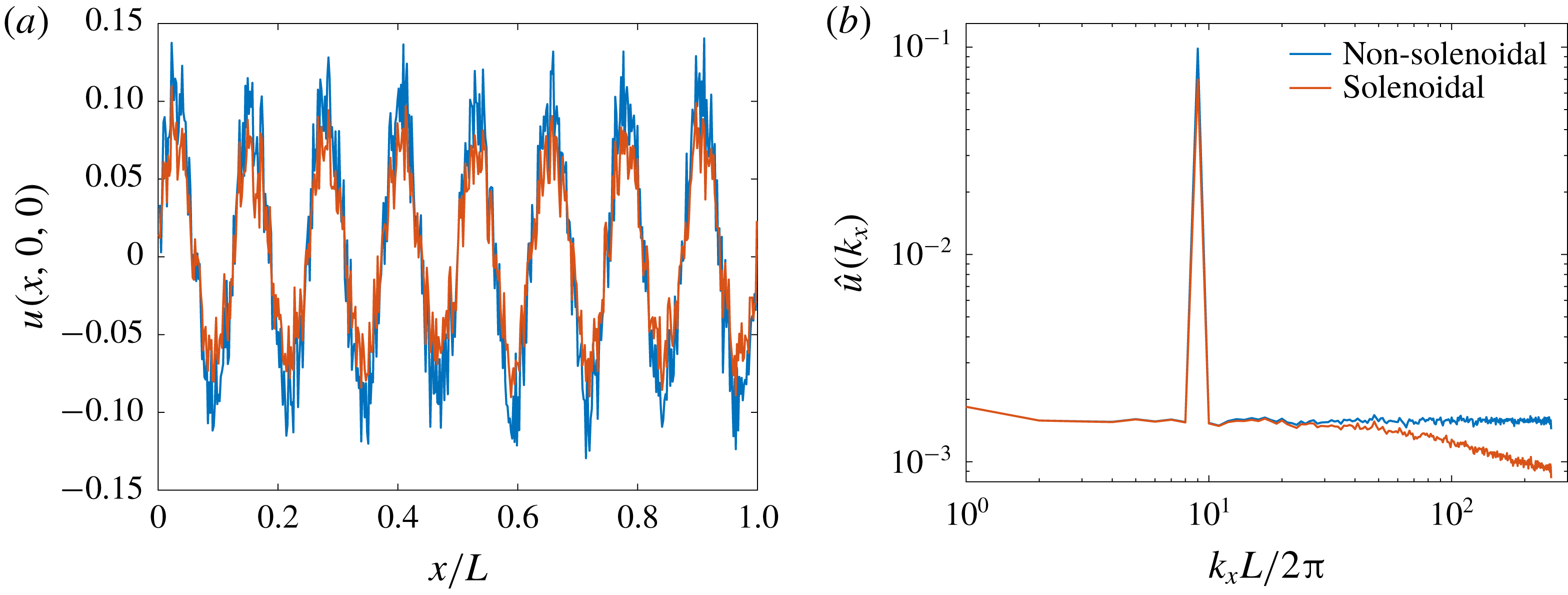
) is independent of perturbation wavenumbers. The projection of (2.3a
)–(2.3c
) onto a solenoidal basis does not influence the forcing wavelength, determined by
 $k_{x}^{0}$
, as discussed in § B.1.
3 Results
3.1 LES validation
Before investigating mixing sensitivity to initial conditions, flow statistics obtained from LES are compared against DNS and experimental results to establish independence of the LES results from boundary condition choices, grid resolution and subgrid-scale model. Shear flow attaining
 $Re_{\unicode[STIX]{x1D6FF}}\approx 3.3\times 10^{4}$
and
 $Re_{\unicode[STIX]{x1D703}}\equiv \unicode[STIX]{x1D703}\unicode[STIX]{x0394}U/\unicode[STIX]{x1D708}\approx 4.0\times 10^{3}$
is considered in this section. An initialization similar to § 2.2 with
 $k_{x}^{0}L=8\unicode[STIX]{x03C0}$
(
 $k_{x}^{0}\unicode[STIX]{x1D703}_{0}=0.025$
) is used for DNS, whereas LES runs are initialized by spectrally filtering and interpolating the DNS solution at
 $t/\unicode[STIX]{x1D70F}=12$
, where the time scale is
 $$\begin{eqnarray}\unicode[STIX]{x1D70F}\equiv \frac{1}{k_{x}^{0}\unicode[STIX]{x0394}U}.\end{eqnarray}$$
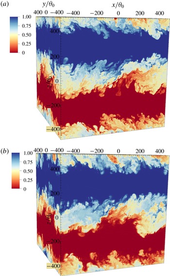
Passive-scalar field at
 $t/\unicode[STIX]{x1D70F}=80$
from (a) DNS using
 $N=2048$
and (b) LES using the stretched-vortex SGS model and
 $N=256$
.

3.1.1 Comparison with DNS at moderate Reynolds number
To compare and assess mixing statistics derived from LES results using the stretched-vortex, constant-coefficient and dynamic-Smagorinsky SGS models (appendix A), a DNS using a pseudospectral solver (Chung & Matheou Reference Chung and Matheou2012) with
 $N=2048$
grid points in each direction is performed.
Figure 1 renders the scalar field at
 $t/\unicode[STIX]{x1D70F}=80$
from the DNS and a LES using the stretched-vortex SGS model. As mentioned in § 2, periodic boundary conditions are used in all three directions. They imply an infinite stack of shear layers in the non-homogeneous direction, each separated initially by a cross-stream distance of
 $L_{z}/2$
. The contours at the top and bottom boundaries in figure 1 show the halves of the mixing layer that develop at a separation of
 $L_{z}/2$
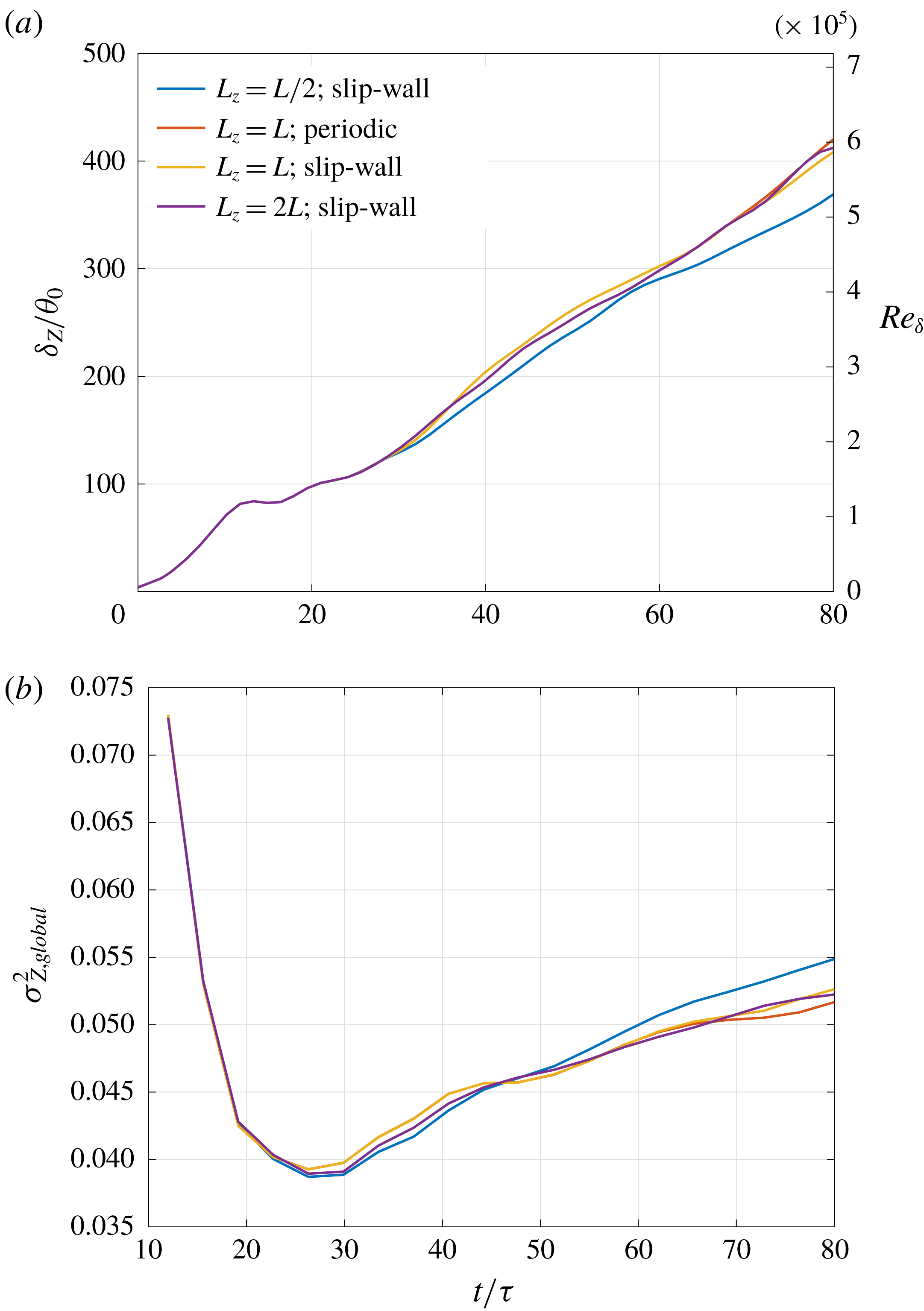
. The separation between the shear layers is large enough to not influence flow statistics from individual shear layers in the time period spanned by our analyses, as confirmed by comparisons against experimental results in § 3.1.2 and § C.2, and by comparisons against simulations using slip-wall cross-stream boundaries in § C.3.

To resolve all scales in different flow phases, the
 $2048^{3}$
grid points required by DNS should be contrasted to the
 $256^{3}$
grid points used for the LES in figure 1, with attendant significant computational cost savings. Flow statistics from the DNS and various LES are compared next.
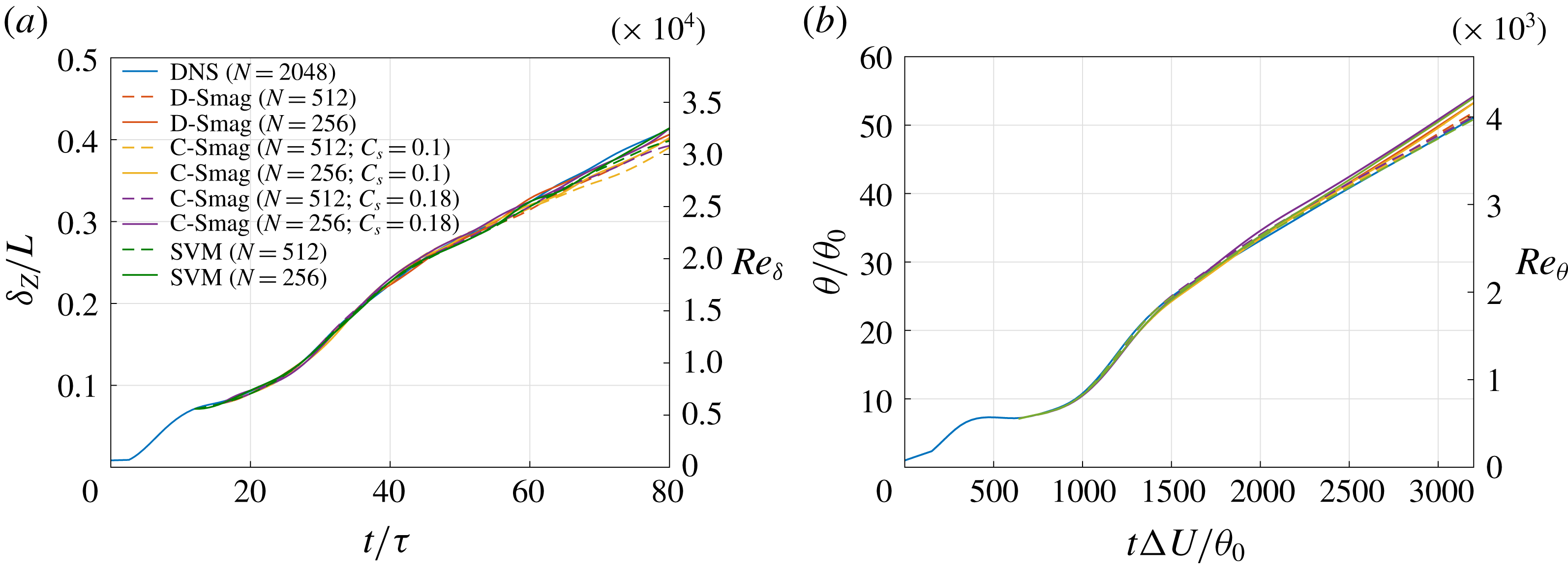
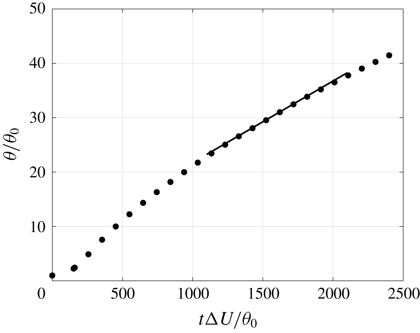
Figure 2(a,b) compares the shear-layer width
 $\unicode[STIX]{x1D6FF}_{Z}$
, representing the
 $1\,\%$
shear-layer mean scalar profile thickness (1.1b
), and the momentum thickness (2.3e
), respectively, versus time between the DNS and LES results from various SGS models at two grid resolutions,
 $N=256$
and
 $N=512$
. The right ordinate axes in the plots show corresponding Reynolds numbers,
 $Re_{\unicode[STIX]{x1D6FF}}$
, where
 $\unicode[STIX]{x1D6FF}=\unicode[STIX]{x1D6FF}_{Z}$
, and
 $Re_{\unicode[STIX]{x1D703}}$
, respectively. Results from the constant-coefficient and dynamic-Smagorinsky SGS models are denoted by ‘C-Smag’ and ‘D-Smag’, respectively, whereas those from the stretched-vortex model are denoted by ‘SVM’.
The shear-layer width and growth in different LES results are in good agreement with DNS results at all times, confirming that large-scale dynamics is not particularly sensitive to choices of subgrid-scale models. The temporal growth rate in the linear region (
 $t\unicode[STIX]{x0394}U/\unicode[STIX]{x1D703}_{0}\gtrsim 2000$
) of figure 2(b), defined as
 $$\begin{eqnarray}r_{\unicode[STIX]{x1D703}}=\frac{\text{d}(\unicode[STIX]{x1D703}/\unicode[STIX]{x1D703}_{0})}{\text{d}(t\unicode[STIX]{x0394}U/\unicode[STIX]{x1D703}_{0})}=\frac{1}{\unicode[STIX]{x0394}U}\frac{\text{d}\unicode[STIX]{x1D703}}{\text{d}t},\end{eqnarray}$$
is
 $0.015$
in the DNS and varies between 0.015 and 0.0165 in various LES cases, in good agreement with the growth rate of
 $0.016$
obtained from Bell & Mehta (Reference Bell and Mehta1990) in the self-similar region of their mixing layer from turbulent (tripped) splitter-plate boundary layers and of
 $0.014$
observed by Rogers & Moser (Reference Rogers and Moser1994) in their temporal mixing layer DNS.
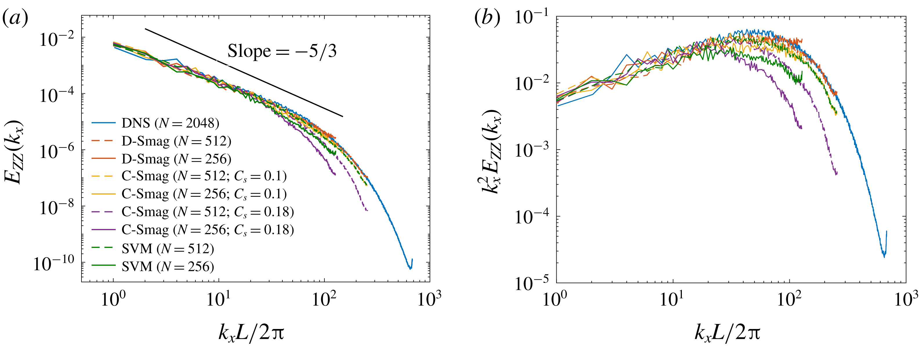
One-dimensional resolved spectra along the streamwise direction on the mixing-layer mid-plane at
 $t/\unicode[STIX]{x1D70F}=80$
from DNS and LES, comparing different SGS models and grid resolutions. (a) Scalar spectra,
 $E_{ZZ}(k_{x})$
(3.3), (b) scalar streamwise-gradient spectra,
 $k_{x}^{2}E_{ZZ}(k_{x})$
.

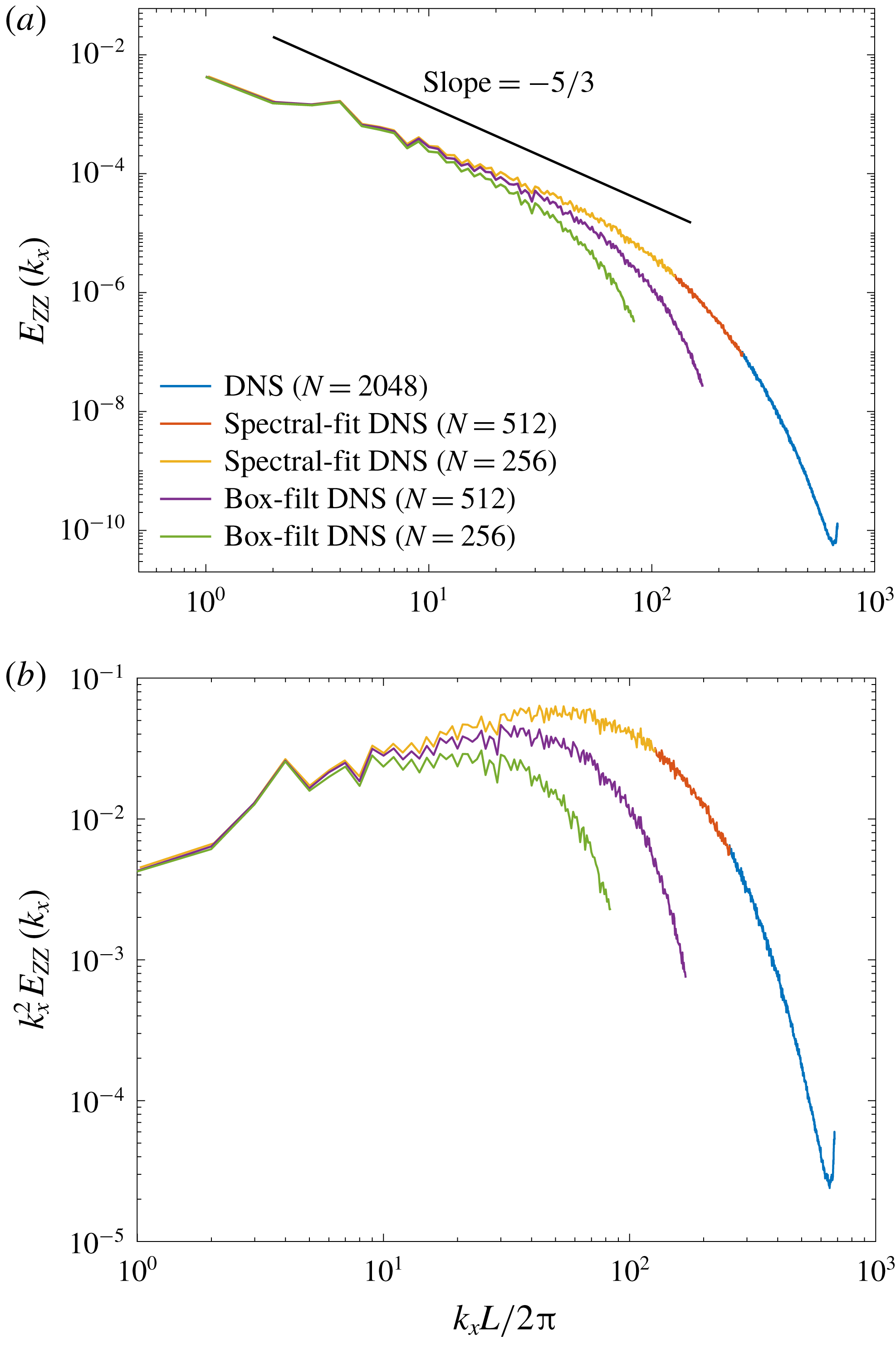
Figure 3 compares one-dimensional spectra of the scalar field,
 $Z(x,y,z)$
, and their streamwise scalar gradients,
 $\unicode[STIX]{x2202}Z(x,y,z)/\unicode[STIX]{x2202}x$
, the latter to illustrate high-wavenumber behaviour. These are computed on the mid-height plane,
 $z=0$
, at
 $t/\unicode[STIX]{x1D70F}=80$
from both DNS and different LES runs. The mid-plane one-dimensional resolved-scalar spectra are calculated as
 $$\begin{eqnarray}E_{ZZ}(k_{x})=\langle |\text{DFT}_{k_{x}}\{Z(x,y,z=0)\}|^{2}\rangle _{y},\end{eqnarray}$$
where
 $\text{DFT}_{k_{x}}\{\cdot \}$
denotes the one-dimensional discrete Fourier transform along the streamwise
 $x$
-direction and
 $\langle \cdot \rangle _{y}$
the average over the spanwise
 $y$
-direction, of the scalar field,
 $Z(\boldsymbol{x},t)$
, from DNS or the resolved-scalar field,
 $\overline{Z}(\boldsymbol{x},t)$
, from LES. Spectra from the higher- and lower-resolution LES runs can be identified by the highest
 $k_{x}$
values depicted.
Figure 3 suggests that, on the basis of spectral power as the criterion, the stretched-vortex model introduces somewhat more dissipation (lower spectral power) than the dynamic-Smagorinsky model, especially at coarser grid resolution, while the dynamic-Smagorinsky model predicts somewhat higher spectral power at high wavenumbers at coarse resolution (figure 3
b), which may be interpreted as entailing lower dissipation at high wavenumbers at coarse resolution. The constant-coefficient Smagorinsky model with coefficients
 $C_{s}=0.1$
and
 $0.18$
is also examined.
 $C_{s}=0.18$
is the theoretical value from the Lilly (Reference Lilly1966a
,Reference Lilly
b
) derivation, assuming that mean kinetic-energy transfer to subgrid scales is balanced by subgrid dissipation and the LES-filter cutoff wavenumber lies in the inertial range with a
 $k^{-5/3}$
Kolmogorov energy cascade and Kolmogorov prefactor of
 $1.4$
.
 $C_{s}=0.1$
, however, provides a better match to the DNS spectrum than
 $C_{s}=0.18$
, as noted for free-shear flows in several previous studies (e.g. Moin & Kim Reference Moin and Kim1982; Lesieur & Metais Reference Lesieur and Metais1996). A turbulent Schmidt number
 $Sc_{T}=1/3$
is assumed with both values of
 $C_{s}$
in the constant-coefficient implementation (Eidson Reference Eidson1985). We will return to these comparisons in the context of mixing predictions below.
A good match of resolved LES spectra to unfiltered DNS spectra is, however, not an appropriate criterion to assess SGS-model performance in LES that does not employ an explicit sharp spectral cutoff filter. LES with grid-filter and finite-difference operators, used commonly in practice and in this work, allow overlap of resolved and subgrid scales. Box-filtered DNS solutions, which possess such characteristics are, therefore, commonly used for comparisons against those LES results.
A box filter with sides of length
 $(2b+1)\unicode[STIX]{x0394}x_{f}$
is considered, where
 $\unicode[STIX]{x0394}x_{f}$
is the grid spacing on the fine DNS grid and
 $b=N_{f}/N_{c}$
is the ratio of number of grid points in each direction on the fine DNS mesh to the coarse LES mesh. This choice of box length allows the fine-grid points to be evenly distributed on both sides of the point where the filtered value is computed (Clark, Ferziger & Reynolds Reference Clark, Ferziger and Reynolds1979). The filtered quantity at a
 $(i,j,k)$
grid coordinate is then given by
 $$\begin{eqnarray}\overline{\unicode[STIX]{x1D719}}_{ijk}=\frac{1}{(2b+1)^{3}}\mathop{\sum }_{i^{\prime }=i-b}^{i+b}\mathop{\sum }_{j^{\prime }=j-b}^{j+b}\mathop{\sum }_{k^{\prime }=k-b}^{k+b}\unicode[STIX]{x1D719}_{i^{\prime }j^{\prime }k^{\prime }}.\end{eqnarray}$$
Differences between box-filtered and sharp cutoff spectrally filtered results with respect to scalar mixing estimates are discussed in § C.1.
The mixed-fluid composition evolution in shear layers can be assessed using the scalar variance about the global mixed-fluid mean concentration as a metric,
 $$\begin{eqnarray}\unicode[STIX]{x27E6}\overline{Z}\unicode[STIX]{x27E7}=\int _{\unicode[STIX]{x1D701}}^{1-\unicode[STIX]{x1D701}}{\mathcal{Z}}{\mathcal{P}}({\mathcal{Z}})\,\text{d}{\mathcal{Z}},\end{eqnarray}$$
with the global scalar variance given by
 $$\begin{eqnarray}\unicode[STIX]{x1D70E}_{Z,global}^{2}=\int _{\unicode[STIX]{x1D701}}^{1-\unicode[STIX]{x1D701}}({\mathcal{Z}}-\unicode[STIX]{x27E6}\overline{Z}\unicode[STIX]{x27E7})^{2}{\mathcal{P}}({\mathcal{Z}})\,\text{d}{\mathcal{Z}},\end{eqnarray}$$
where
 ${\mathcal{P}}({\mathcal{Z}})$
is the resolved-scalar p.d.f. A value of
 $\unicode[STIX]{x1D701}=1/25$
is used as a threshold between mixed and unmixed fluid. The local scalar variance,
 $\unicode[STIX]{x1D70E}_{Z,local}^{2}$
, representing local scalar fluctuations or physical stirring/dispersion of fluid elements, about the local mean can be obtained by substituting
 $\unicode[STIX]{x27E6}\overline{Z}\unicode[STIX]{x27E7}$
in (3.5b
) with the local or spatially varying mean,
 $\langle \overline{Z}\rangle$
(e.g. Sharan et al.
Reference Sharan, Matheou and Dimotakis2018a
).
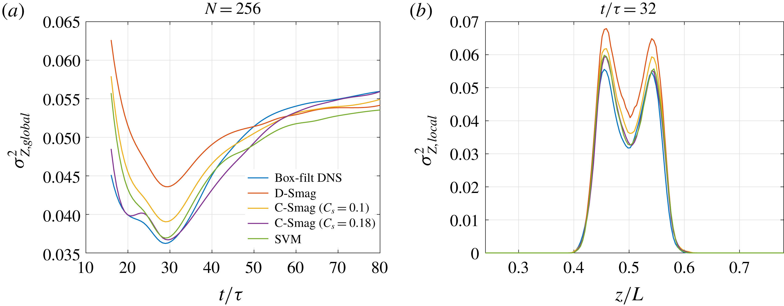
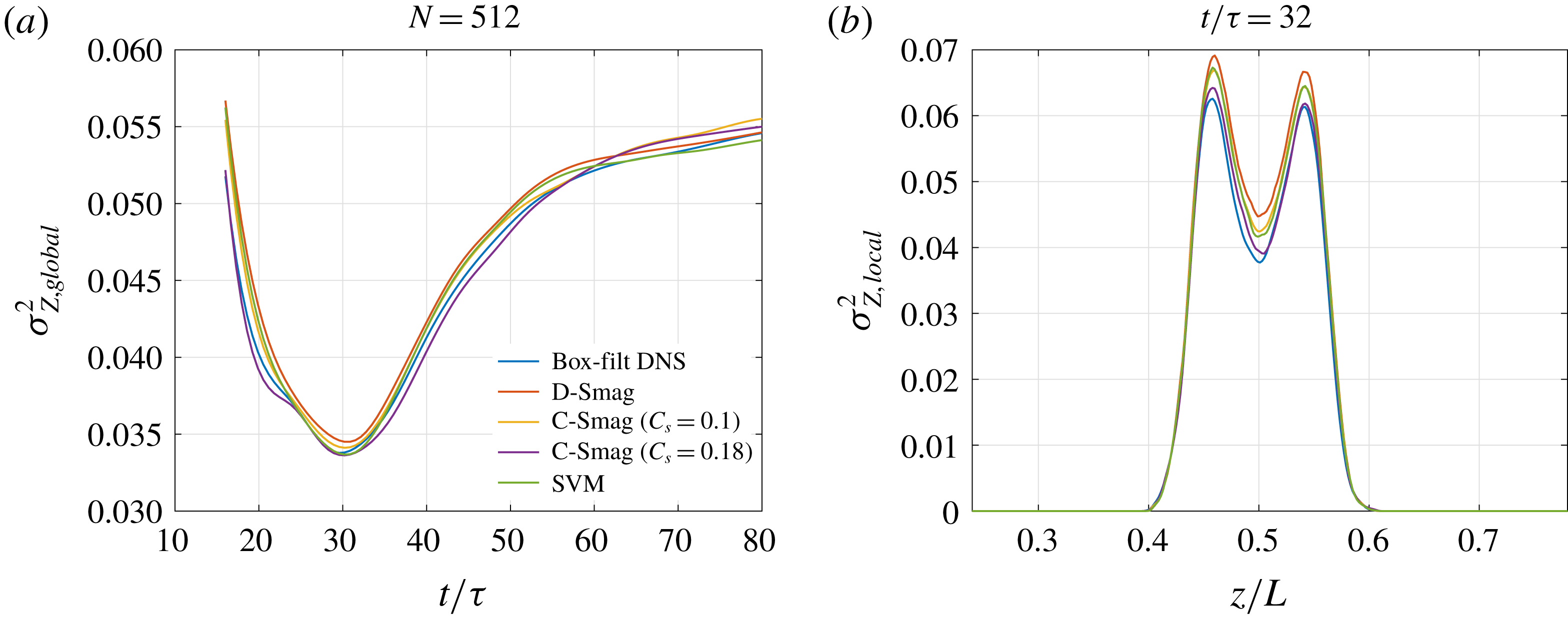
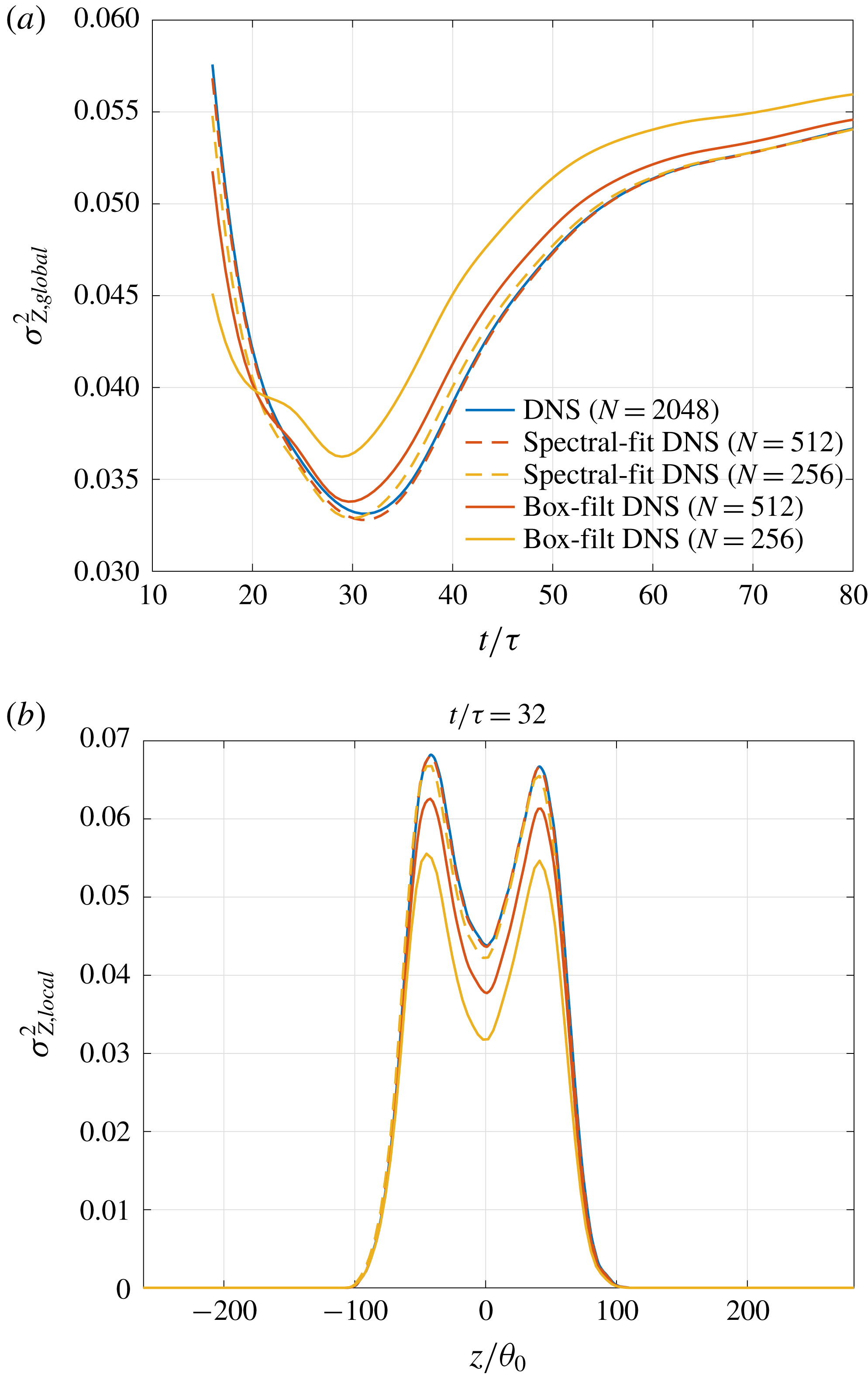
Figures 4 and 5 compare the global and local scalar variance between box-filtered DNS estimates and resolved estimates from LES using various SGS models, with
 $N=256$
and
 $N=512$
, respectively, to help assess the role of grid resolution in LES mixing predictions.


The local scalar variance is plotted at
 $t/\unicode[STIX]{x1D70F}=32$
, near the time of the global scalar-variance minimum, when results are found to be sensitive to the choice of the SGS model. Differences in mixed-fluid composition and scalar fluctuations from various SGS models is more clearly seen in figure 4, which shows the coarser-grid results. The time of global scalar variance minimum is well-predicted by all SGS models employed. The box-filtered DNS results are closest to the LES results from the stretched-vortex and the constant-coefficient Smagorinsky model with
 $C_{s}=0.18$
, while the dynamic-Smagorinsky results in the coarse (
 $N=256$
) LES are the farthest from the filtered-DNS results.
Resolved-variable statistics are sensitive to filter choice and, therefore, agreements with box-filtered DNS results, though commonly reported in the literature, may not necessarily imply SGS-model robustness in LES using implicit filtering. An alternative SGS-model assessment can be performed by adding subgrid estimates to the resolved LES estimates to obtain total values and comparing them against the unfiltered DNS results.
(a) Total,
 $\unicode[STIX]{x1D70E}_{Z,tot}^{2}$
(C 6a
), and subgrid,
 $\unicode[STIX]{x1D70E}_{Z,sgs}^{2}$
(C 8c
), scalar variance. (b) Total,
 $\unicode[STIX]{x1D700}_{tot}$
(C 7a
), and subgrid,
 $\unicode[STIX]{x1D700}_{sgs}$
(C 8b
), dissipation from DNS and LES using the stretched-vortex SGS model.
 $N$
denotes the number of grid points in each direction. Legend is the same for both plots.

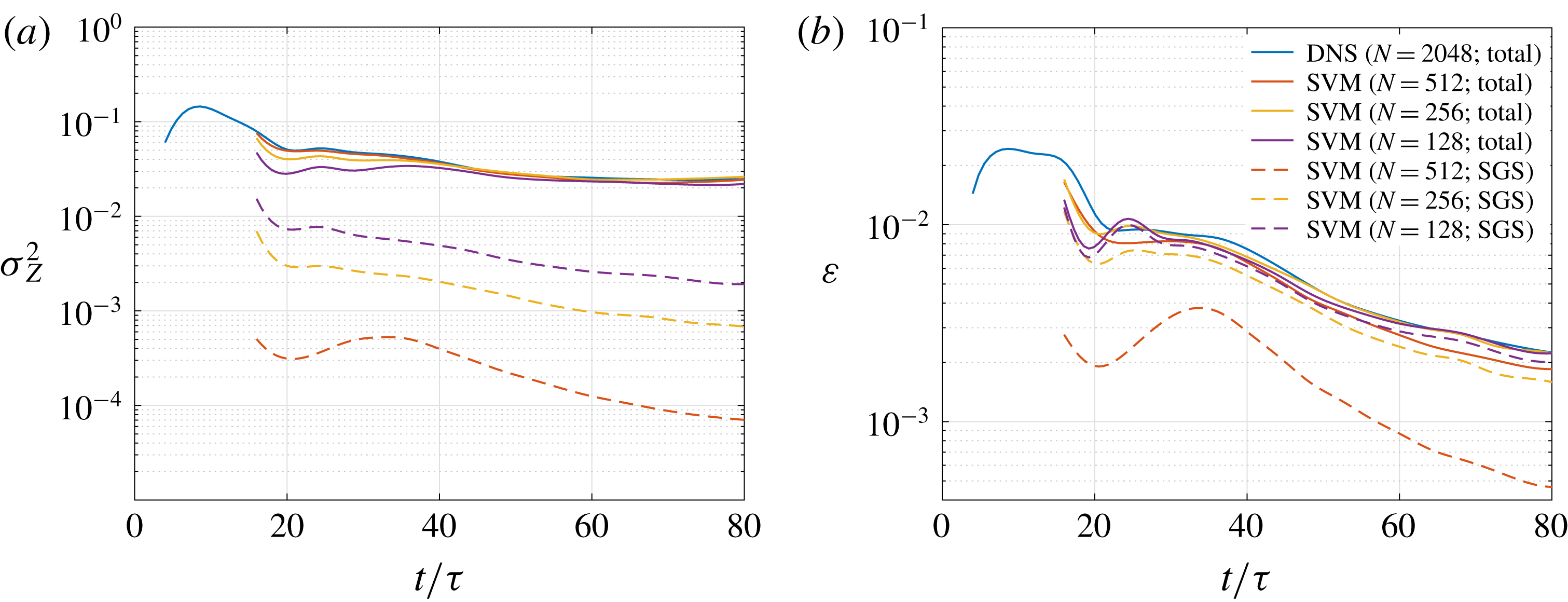
Figure 6 compares the total scalar variance and dissipation, labelled ‘Total’, between DNS and LES using the stretched-vortex SGS model at different grid resolutions. Subgrid contributions, labelled ‘SGS’, are calculated as described in § C.5.
After the initial laminar and transition stages, total scalar-variance estimates from different LES are seen to be in good agreement with the DNS, as evident from the solid lines in figure 6(a). Total dissipation estimates, shown in figure 6(b), from the LES using
 $N=128$
and
 $N=256$
are in good agreement with the DNS, while the estimates from
 $N=512$
are slightly lower. The minor discrepancy at
 $N=512$
is likely a result of a less accurate subgrid dissipation estimate at this grid resolution, where grid spacing is not much larger than the local Kolmogorov length and the filter cutoff wavenumber may not lie in the inertial range, atypical for LES.
As expected, the subgrid contribution to the total scalar variance and dissipation decreases with increases in grid resolution, as seen in figure 6. Importantly in the context of and focus on mixing in the present discussion, subgrid dissipation typically accounts for nearly all dissipation and mixing estimates in a practical LES. However, to allow comparisons with DNS, a moderate-
 $Re_{\unicode[STIX]{x1D6FF}}$
flow was considered in this section, in which resolved dissipation is significant, especially at
 $N=512$
.
In § 3.2, we consider high-
 $Re_{\unicode[STIX]{x1D6FF}}$
shear flows, which have negligible resolved dissipation, to assess the initial perturbation influence on mixing and p.d.f. characteristics. Results from LES using the stretched-vortex SGS model are discussed in § 3.2 because of good agreement of their total (resolved + subgrid) statistics with DNS, as shown above, and good agreement of their self-similar mean velocity profile and Reynolds stresses with Bell & Mehta (Reference Bell and Mehta1990) experimental results, as discussed in the next section and § C.2.
3.1.2 Comparison with experiment
The initial condition (2.3) influences vortex amalgamations in the early stages of flow development, as discussed in the next section, resulting in nonlinear shear-layer growth at early times, as shown in figure 2. However, after
 $t/\unicode[STIX]{x1D70F}\gtrsim 50$
or
 $t\unicode[STIX]{x0394}U/\unicode[STIX]{x1D703}_{0}\gtrsim 2000$
, the shear layer grows approximately linearly with time suggesting self-similar evolution at late times. Self-similarity may also be inferred from an approximately constant total scalar variance and dissipation around
 $t/\unicode[STIX]{x1D70F}\approx 60$
in figure 6. Flow statistics in the self-similar region can be compared with experimental results for simulation validation.
The Bell & Mehta (Reference Bell and Mehta1990) experimental results are commonly used for comparisons. See Rogers & Moser (Reference Rogers and Moser1994), Balaras et al. (Reference Balaras, Piomelli and Wallace2001), Pantano & Sarkar (Reference Pantano and Sarkar2002) and Mattner (Reference Mattner2011), for example. As noted in the previous section, the momentum thickness growth rate (3.2) from LES, calculated at late times from figure 2(b), is in good agreement with the Bell & Mehta results.
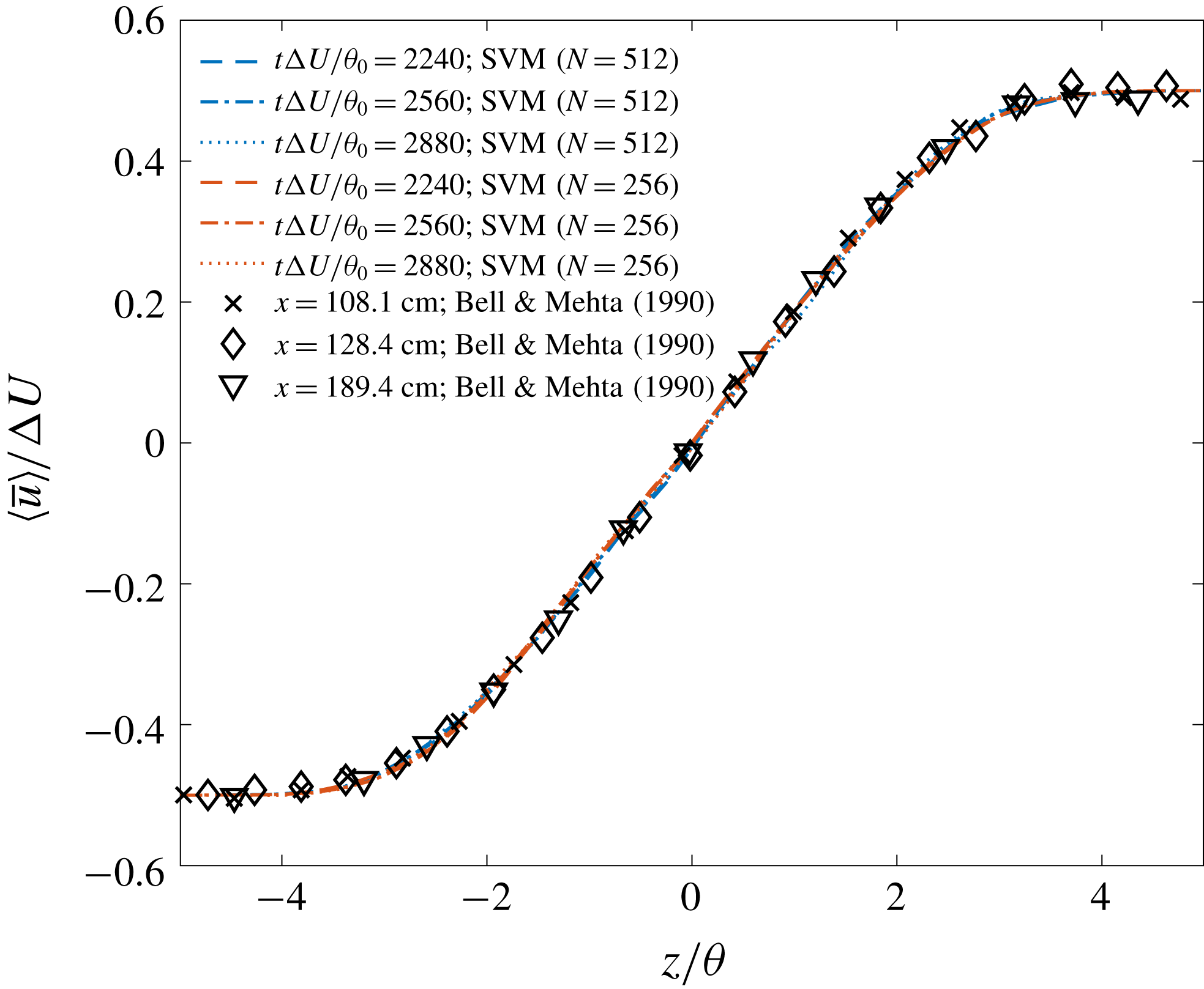
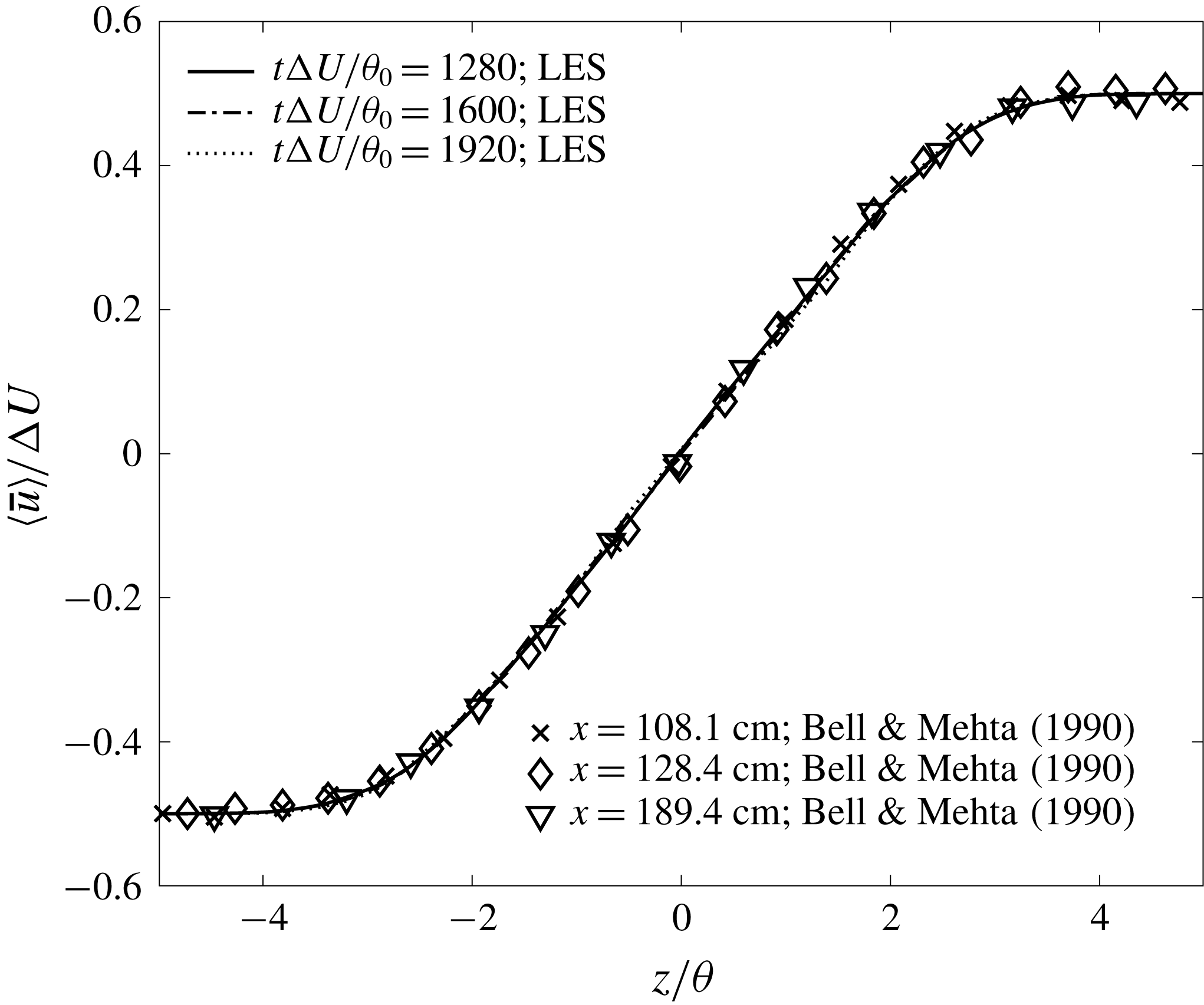
Figure 7 shows the mean streamwise velocity profile in similarity coordinates,
 $z/\unicode[STIX]{x1D703}$
, at
 $t\unicode[STIX]{x0394}U/\unicode[STIX]{x1D703}_{0}$
of
 $2240$
,
 $2560$
and
 $2880$
(
 $t/\unicode[STIX]{x1D70F}$
of
 $56$
,
 $64$
and
 $72$
) from LES using the stretched-vortex SGS model with
 $N=256$
and
 $512$
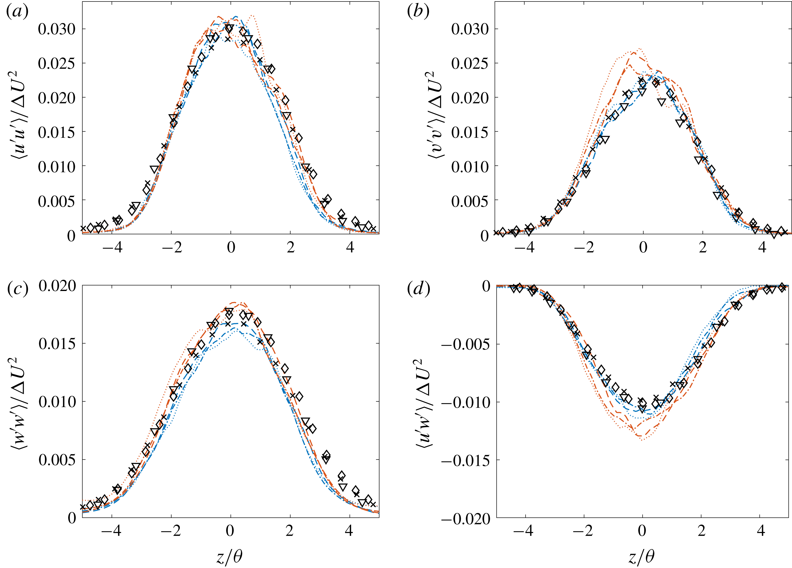
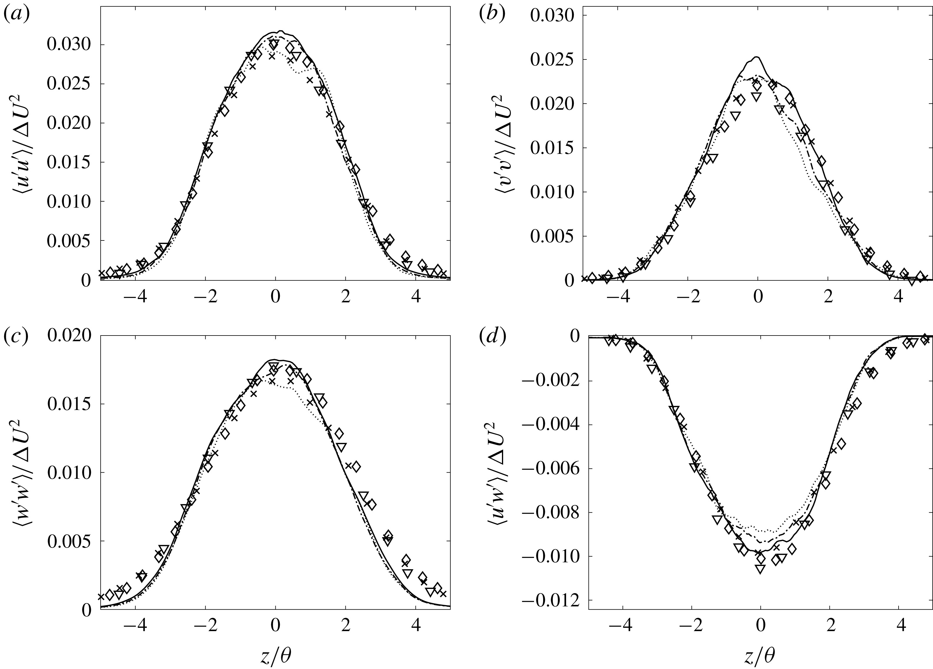
. The markers show the Bell & Mehta experimental results at three axial distances of their mixing layer from turbulent (tripped) splitter-plate boundary layers. LES results are in good agreement with the Bell & Mehta profile. Figure 8 compares the components of the Reynolds stresses in similarity coordinates. The Reynolds stresses from the LES are estimated by (e.g. Mattner Reference Mattner2011)
 $$\begin{eqnarray}\langle u_{i}^{\prime }u_{j}^{\prime }\rangle \approx \langle \bar{u}_{i}^{\prime }\bar{u}_{j}^{\prime }\rangle +\langle \unicode[STIX]{x1D70F}_{ij}\rangle ,\end{eqnarray}$$
where
 $\bar{u}_{i}^{\prime }=\bar{u}_{i}-\langle \bar{u}_{i}\rangle$
and
 $\unicode[STIX]{x1D70F}_{ij}$
denotes the SGS stress (A 1a
). The collapse of the LES Reynolds stress profiles at various times indicates self-similarity at late times in the flow. The stresses also compare fairly well with the Bell & Mehta self-similar profiles, despite differences in flow initialization.
Further validation of the present computational set-up and LES using the stretched-vortex SGS model for mixing layer from a three-dimensional initial perturbations resembling turbulent inflow in experimental studies is discussed in § C.2.
To summarize this section, mixing-layer statistics from LES using the stretched-vortex SGS model show good agreement with DNS as well as with experimental results. Results from LES using the stretched-vortex SGS model are, therefore, discussed in the next section. The conclusions of the study, however, are independent of SGS-model choices investigated.
Mean streamwise velocity in similarity coordinates from LES using the stretched-vortex SGS model compared against the experimental result of Bell & Mehta (Reference Bell and Mehta1990).

Components of the Reynolds stress tensor in similarity coordinates, compared against experimental result of Bell & Mehta (Reference Bell and Mehta1990). Legend as in the Figure 7 inset.

3.2 Mixing sensitivity to initial perturbations
Shear-flow large-eddy simulations attaining
 $Re_{\unicode[STIX]{x1D6FF}}\approx 5\times 10^{5}$
and
 $Re_{\unicode[STIX]{x1D703}}\approx 7.5\times 10^{4}$
, with initial conditions as in § 2.2 and
 $N=512$
, are discussed in this section.
3.2.1 Effect of streamwise forcing
Initial perturbations, given by the square brackets in (2.3a–c ), mimic forced perturbations employed in the experimental studies of spatially developing mixing layers by Oster & Wygnanski (Reference Oster and Wygnanski1982) using an oscillating flap and by Ho & Huang (Reference Ho and Huang1982) using butterfly valves. Qualitative comparisons against experimental results are discussed below. Unfortunately, lack of self-similarity until late times in purposely perturbed flows, as described below, and insufficient details to precisely reconstruct functional forms of initial profiles render direct quantitative comparisons largely infeasible in the flow stages of interest here.
Evolution of shear-layer width from different initial conditions plotted against time non-dimensionalized using (a) the initial momentum thickness,
 $\unicode[STIX]{x1D703}_{0}$
, and (b) the reciprocal of perturbation wavenumber
 $k_{x}^{0}$
as length scale. Legend is the same for both plots.

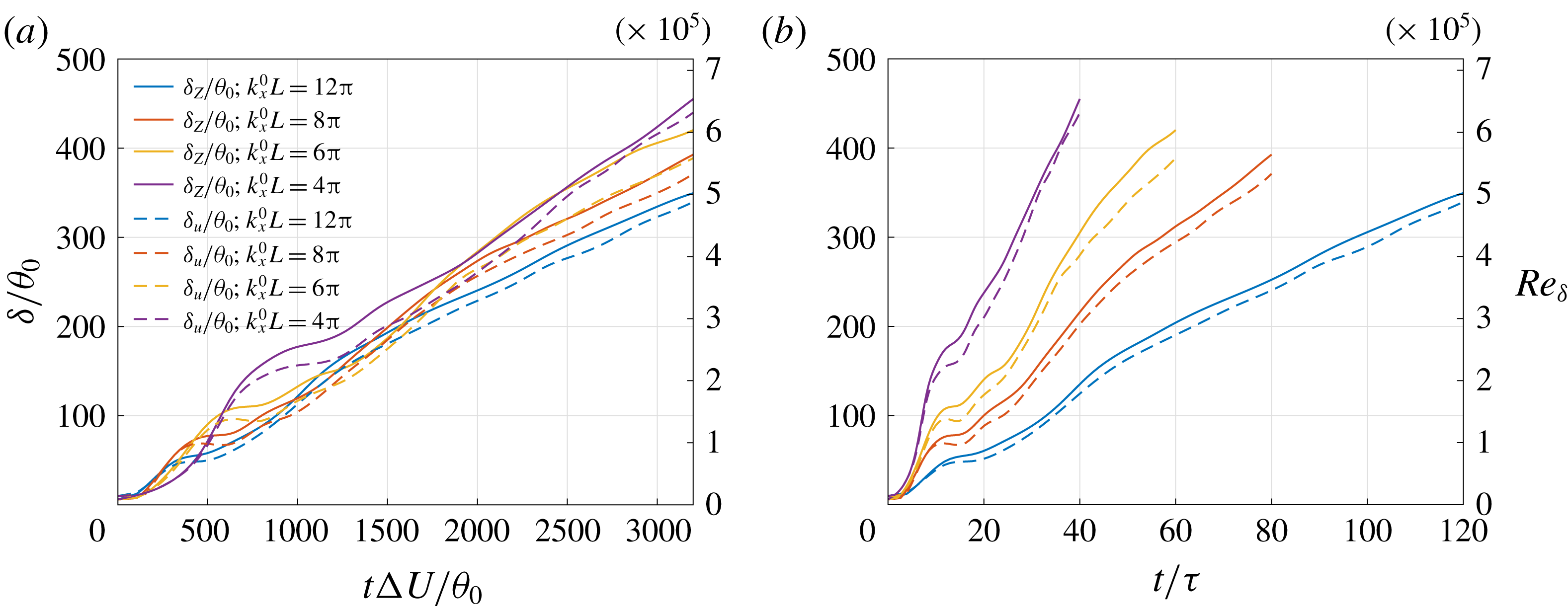
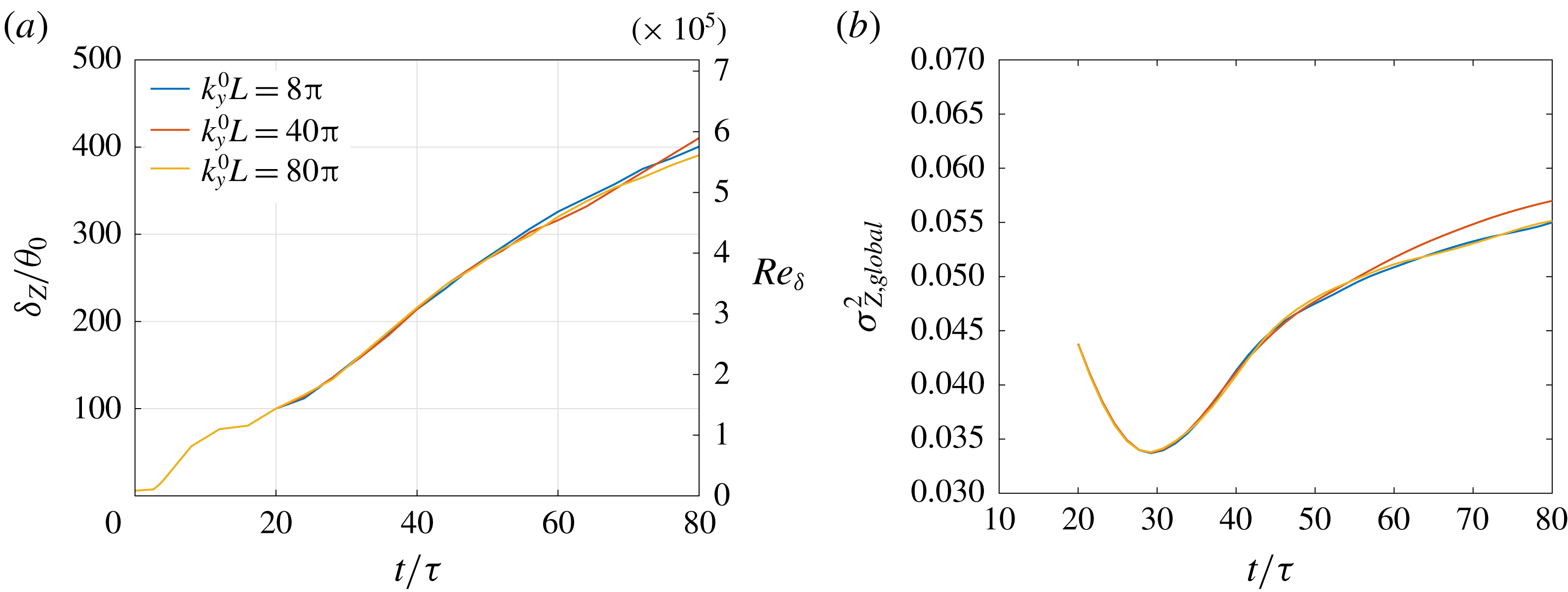
Figure 9 shows the shear-layer width and corresponding Reynolds number with time, as evolved from various values of perturbation wavenumber
 $k_{x}^{0}$
. The wavenumbers are an order of magnitude smaller than the most unstable wavenumber, based on the Oster & Wygnanski study, where the forcing frequency was chosen to be at least an order of magnitude lower than the most unstable frequency to study the inflow influence far downstream. The width based on scalar concentration, denoted
 $\unicode[STIX]{x1D6FF}_{Z}$
, is defined in (1.1b
). The width based on streamwise velocity, denoted
 $\unicode[STIX]{x1D6FF}_{u}$
, is defined as the thickness corresponding to
 $-0.49\leqslant \langle \overline{u}\rangle /\unicode[STIX]{x0394}U\leqslant 0.49$
. In agreement with observations of Oster & Wygnanski (Reference Oster and Wygnanski1982, figures 10 and 13), the width does not grow linearly with time, exhibiting distinct stages with varying growth, Further, a decrease in perturbation wavenumber enhances shear-layer growth. The width based on scalar concentration is slightly larger than that based on streamwise velocity at all times. Growths based on either metric, however, are similar to each other for each initial perturbation.
Shear-layer width non-dimensionalized with
 $t\unicode[STIX]{x0394}U$
, plotted against non-dimensional time
 $t/\unicode[STIX]{x1D70F}$
. Legend as in figure 9(a).

Oster & Wygnanski categorized the streamwise development of their spatially evolving shear flow, attaining
 $Re_{\unicode[STIX]{x1D703}}\approx 10^{4}$
, into three regions/stages, where the spatial location of the stages depended on oscillating-flap frequency. Similar stages are observed with respect to time in figures 2 and 9, at moderate and high Reynolds numbers, respectively.
In figure 9(b), the characteristic time
 $\unicode[STIX]{x1D70F}=1/(k_{x}^{0}\unicode[STIX]{x0394}U)$
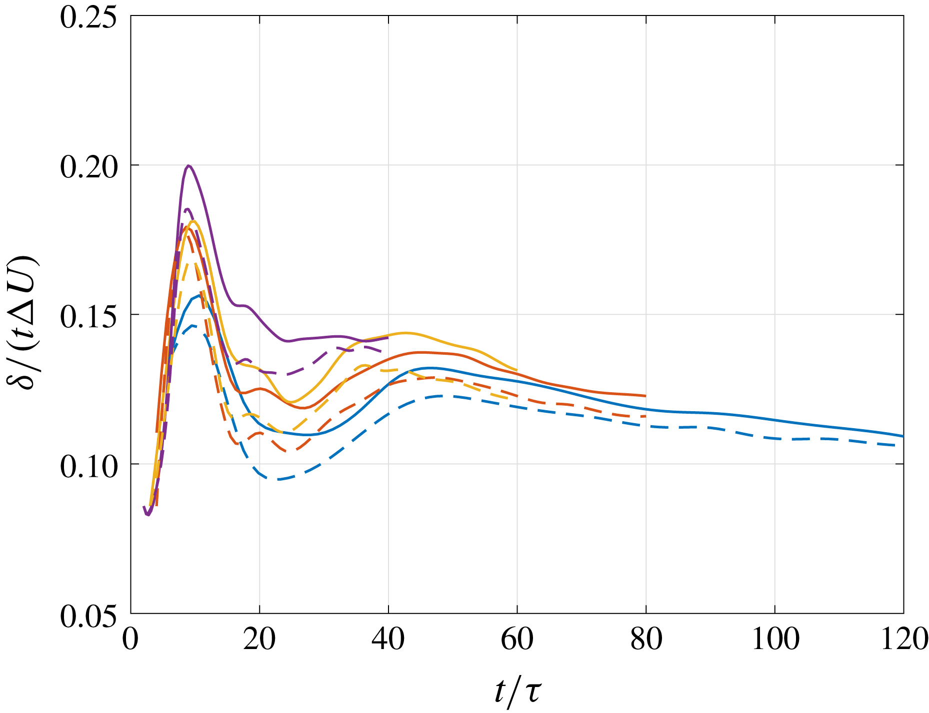
is seen to scale the time evolution of stages, independently of perturbation wavenumber. Various successive stages can be distinctly identified in figure 10 that shows shear-layer widths non-dimensionalized using a length based on Lagrangian time, i.e.
 $t\unicode[STIX]{x0394}U$
, as the appropriate scaling length in the shear-layer convective frame. This figure also illustrates the deviation of shear-layer widths from those of an unforced shear layer that would grow linearly with time and would be represented by a horizontal line in such a plot.
Following the description of Oster & Wygnanski in the context of the temporal shear layers considered here, the first stage,
 $t/\unicode[STIX]{x1D70F}\lesssim 10$
, exhibits increasing growth, which is amplified by a decrease in perturbation wavenumber. Growth decreases in the second stage,
 $10\lesssim t/\unicode[STIX]{x1D70F}\lesssim 30$
, before stagnating at a value that is higher for smaller perturbation wavenumbers. Increases in shear-layer growth coincide with vortex-amalgamation times. Limitations in streamwise extent of the Oster & Wygnanski experimental test section prevented investigation of flow development beyond the third stage, where growth increases. The computations described here allow vortex mergers in the third stage,
 $30\lesssim t/\unicode[STIX]{x1D70F}\lesssim 45$
, resulting in an increase in growth and subsequent evolution to a fourth stage, for
 $t/\unicode[STIX]{x1D70F}\gtrsim 45$
, where growth slowly decreases, becoming approximately linear over some time intervals.
Resolved streamwise turbulence intensity from different initial conditions at (a)
 $t/\unicode[STIX]{x1D70F}\approx 6$
, (b)
 $t/\unicode[STIX]{x1D70F}\approx 18$
and (c)
 $t/\unicode[STIX]{x1D70F}\approx 40$
. Legend is the same for all plots.

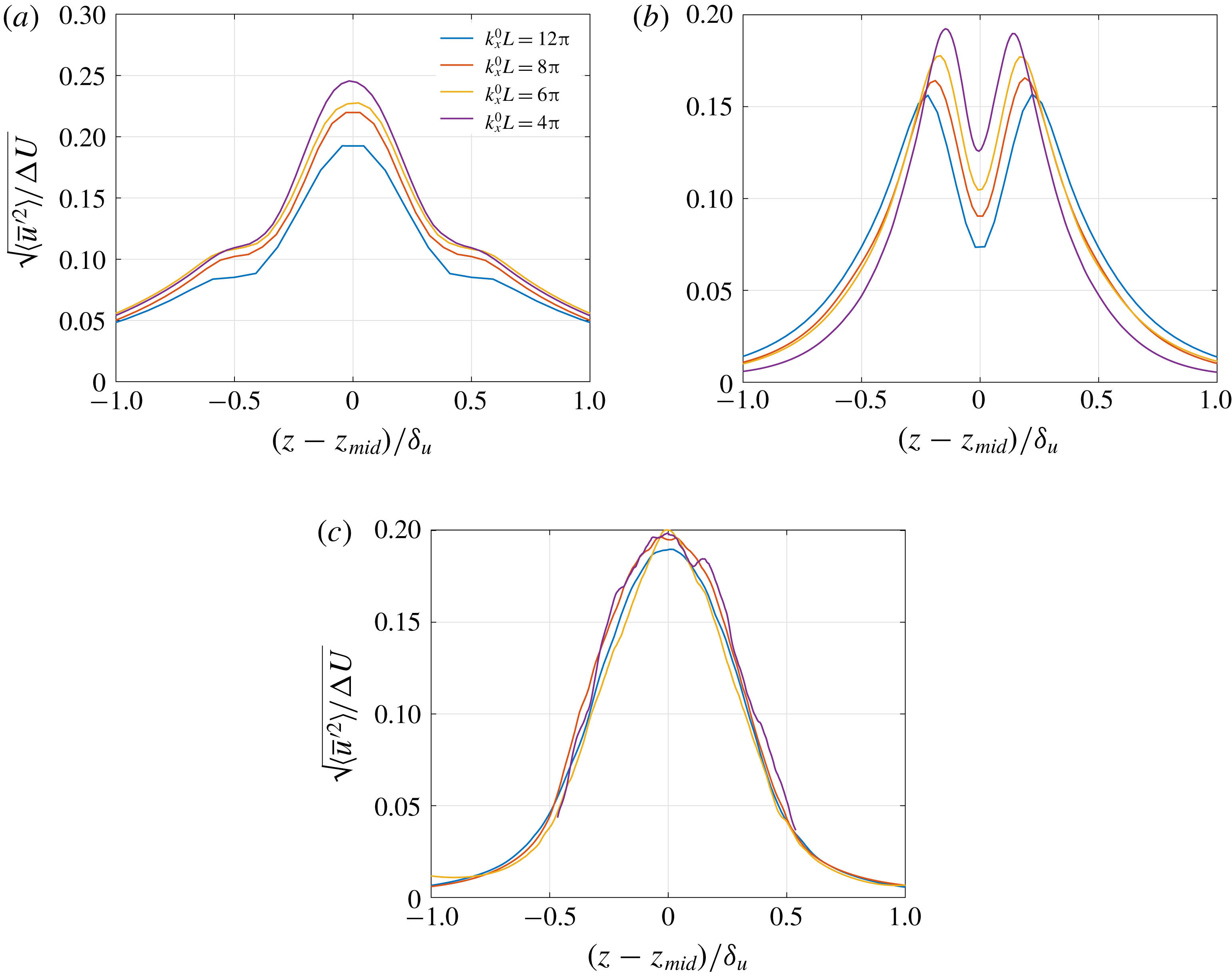
Flow evolution from one stage to another is characterized by a change in the distribution of the resolved streamwise-velocity mean-square fluctuation level,
 $\langle \overline{u}^{\prime 2}\rangle ^{1/2}/\unicode[STIX]{x0394}U$
, where
 $\overline{u}^{\prime }=\overline{u}-\langle \overline{u}\rangle$
is the resolved streamwise velocity fluctuation. As shown in figure 11, the evolution exhibits a single peak in the first stage (
 $t/\unicode[STIX]{x1D70F}\approx 6$
), a double peak in the second stage (
 $t/\unicode[STIX]{x1D70F}\approx 18$
), followed by a single peak in the third stage (
 $t/\unicode[STIX]{x1D70F}\approx 40$
), consistent with the experimental observations of Oster & Wygnanski. In all stages, the peak intensity with a lower-wavenumber initial perturbation is higher. Differences, however, decrease with time.
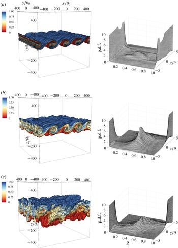
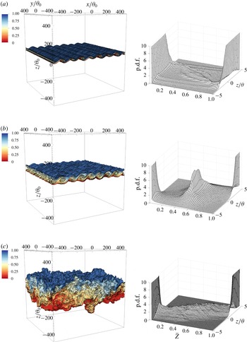
Scalar isosurfaces around the mid-plane (left column) and resolved-scalar p.d.f. (right column) at (a)
 $t\unicode[STIX]{x0394}U/\unicode[STIX]{x1D703}_{0}=800$
(
 $t/\unicode[STIX]{x1D70F}=10$
), (b)
 $t\unicode[STIX]{x0394}U/\unicode[STIX]{x1D703}_{0}=1600$
(
 $t/\unicode[STIX]{x1D70F}=20$
) and (c)
 $t\unicode[STIX]{x0394}U/\unicode[STIX]{x1D703}_{0}=3200$
(
 $t/\unicode[STIX]{x1D70F}=40$
) from an initial condition with
 $k_{x}^{0}L=4\unicode[STIX]{x03C0}$
(
 $k_{x}^{0}\unicode[STIX]{x1D703}_{0}=0.0125$
) in (2.3).

Mixing at various stages of shear-flow development, described above, can be assessed on the basis of scalar statistics.
Figures 12 and 13 show scalar isosurfaces around the mid-plane and the scalar p.d.f. at different stages with
 $k_{x}^{0}L=4\unicode[STIX]{x03C0}$
and
 $8\unicode[STIX]{x03C0}$
(
 $k_{x}^{0}\unicode[STIX]{x1D703}_{0}=0.0125$
and
 $0.025$
), respectively. In the first stage, shown in figures 12(a) and 13(a), two-dimensional spanwise Kelvin–Helmholtz rollers develop whose size and count in the computational domain is determined by
 $k_{x}^{0}$
. These rollers undergo pairings that subsequently induce transition to turbulence (Moser & Rogers Reference Moser and Rogers1993). The initial roll-up entrains pure fluid from the two free streams through the Biot–Savart induced velocity (e.g. Roshko Reference Roshko1976; Dimotakis Reference Dimotakis1986).
Scalar isosurfaces around the mid-plane (left column) and resolved-scalar p.d.f. (right column) at (a)
 $t\unicode[STIX]{x0394}U/\unicode[STIX]{x1D703}_{0}=320$
(
 $t/\unicode[STIX]{x1D70F}=8$
), (b)
 $t\unicode[STIX]{x0394}U/\unicode[STIX]{x1D703}_{0}=800$
(
 $t/\unicode[STIX]{x1D70F}=20$
) and (c)
 $t\unicode[STIX]{x0394}U/\unicode[STIX]{x1D703}_{0}=3200$
(
 $t/\unicode[STIX]{x1D70F}=80$
) from an initial condition with
 $k_{x}^{0}L=8\unicode[STIX]{x03C0}$
(
 $k_{x}^{0}\unicode[STIX]{x1D703}_{0}=0.025$
) in (2.3).

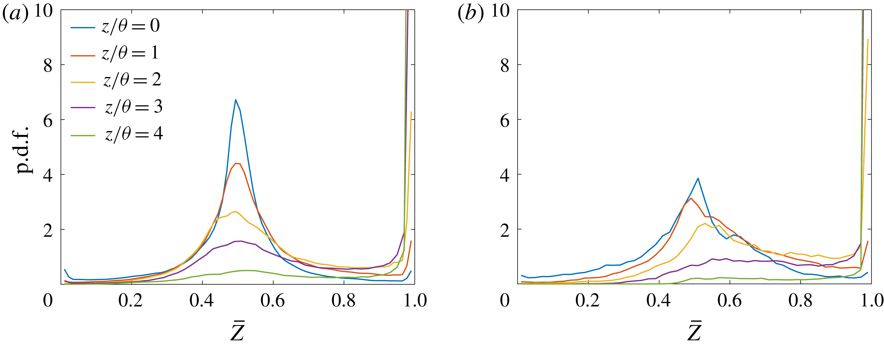
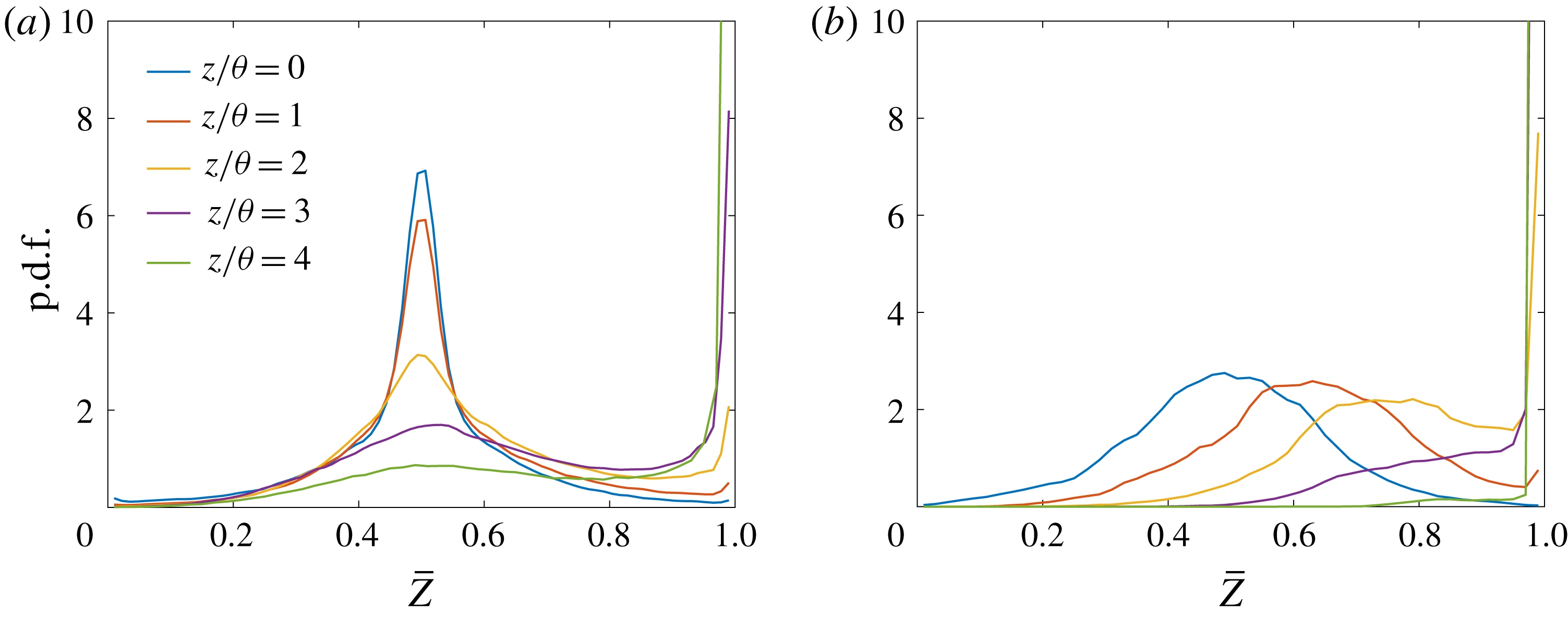
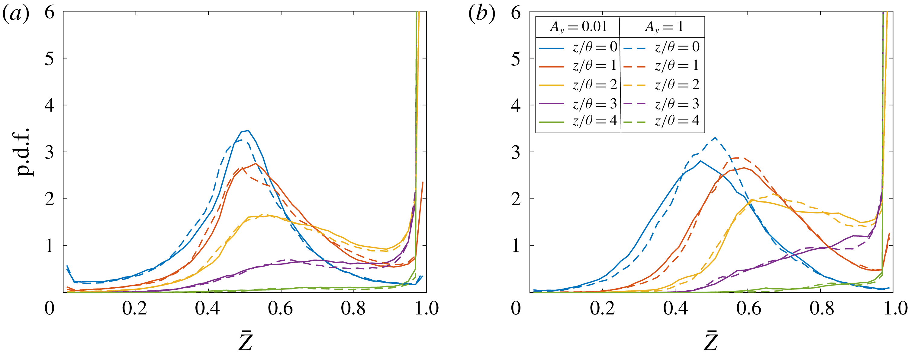
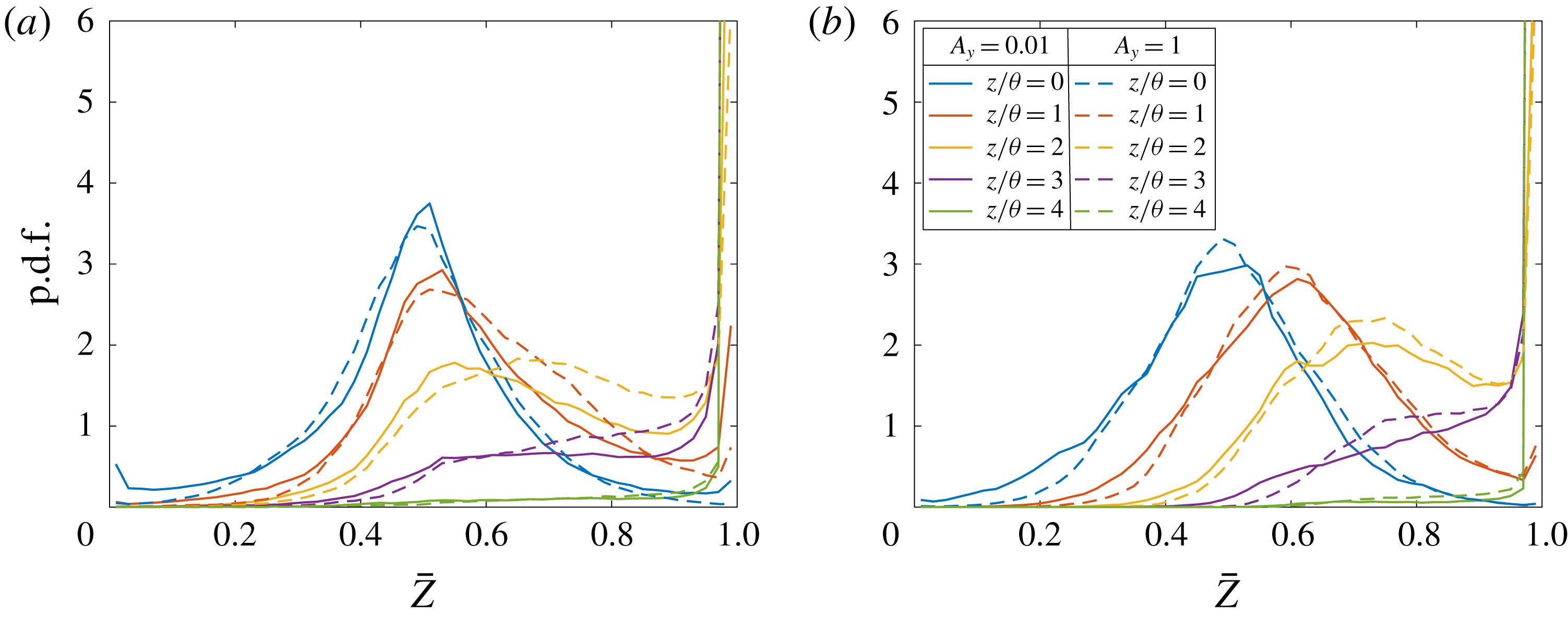
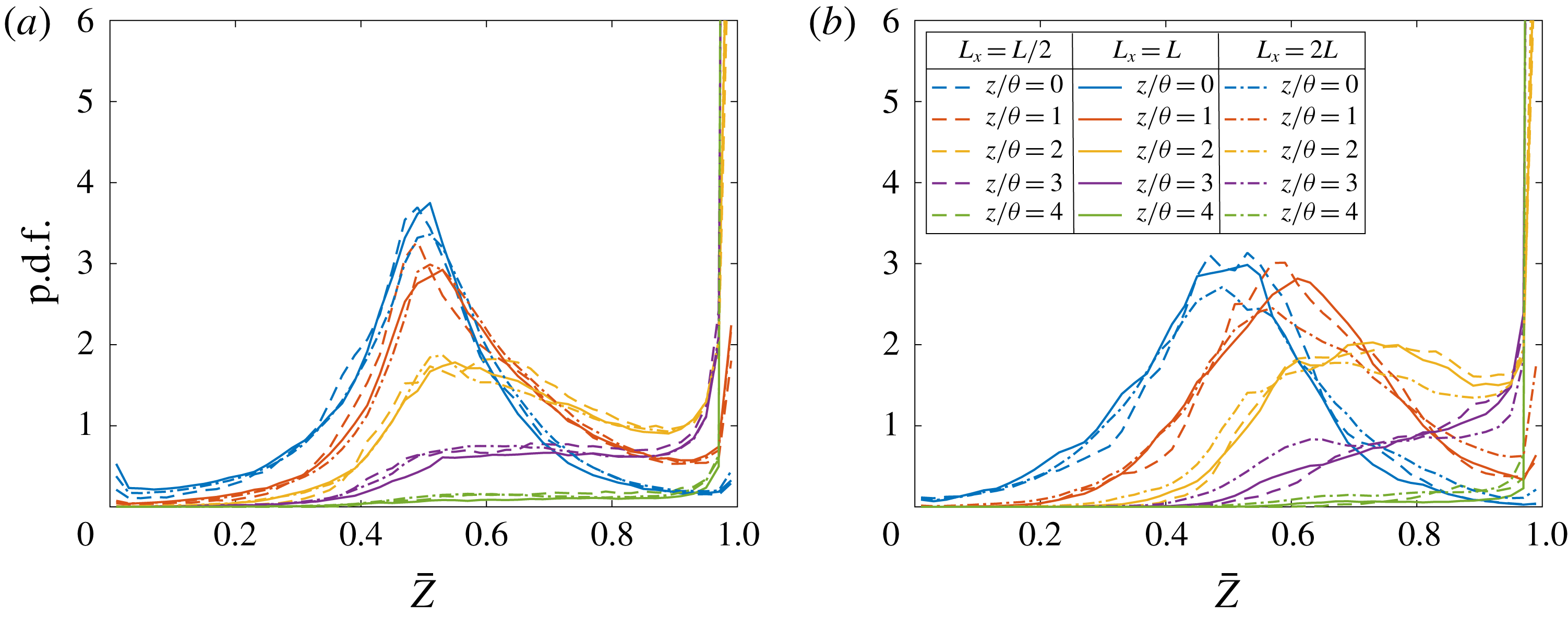
Entrained fluid that is drawn into the shear layer can survive unmixed, as shown in the p.d.f. in figures 12(a) and 13(a). Large vortical structures strain the entrained fluid to generate finer, high-wavenumber structures that are eventually mixed through diffusion, resulting in a nearly uniform composition across the shear layer, or a non-marching p.d.f. in the second stage, as shown in figures 12(b) and 13(b). P.d.f. values are more clearly seen in the line plots at equally spaced cross-stream locations, as shown in figures 14(a) and 15(a) for the two initial conditions at various
 $z/\unicode[STIX]{x1D703}\geqslant 0$
locations. P.d.f. profiles from the other side of the layer (
 $z/\unicode[STIX]{x1D703}<0$
) are statistically symmetric, as expected for this flow.
Mixed-fluid composition is symmetric in this case, because we have uniform-density flow with equal (and opposite) free-stream velocity magnitudes. Shear-layer width grows with time as fluid is continuously entrained, and the p.d.f. transitions from non-marching to marching in due course. At
 $t\unicode[STIX]{x0394}U/\unicode[STIX]{x1D703}_{0}=3200$
, as shown in figures 12(c) and 13(c), the flow with
 $k_{x}^{0}L=4\unicode[STIX]{x03C0}$
(
 $k_{x}^{0}\unicode[STIX]{x1D703}_{0}=0.0125$
) is in the third stage, since
 $t/\unicode[STIX]{x1D70F}=40$
, and exhibits a non-marching p.d.f. on the verge of transition, whereas the flow with
 $k_{x}^{0}L=8\unicode[STIX]{x03C0}$
(
 $k_{x}^{0}\unicode[STIX]{x1D703}_{0}=0.025$
) is in the fourth stage and exhibits a marching p.d.f. Figures 14(b) and 15(b) show the line plots of the p.d.f. at those times for the two initial conditions.
Resolved-scalar p.d.f.s at various cross-stream locations from an initial condition with
 $k_{x}^{0}L=4\unicode[STIX]{x03C0}$
(
 $k_{x}^{0}\unicode[STIX]{x1D703}_{0}=0.0125$
) in (2.3) at (a)
 $t\unicode[STIX]{x0394}U/\unicode[STIX]{x1D703}_{0}=1600$
(
 $t/\unicode[STIX]{x1D70F}=20$
) and (b)
 $t\unicode[STIX]{x0394}U/\unicode[STIX]{x1D703}_{0}=3200$
(
 $t/\unicode[STIX]{x1D70F}=40$
).

Resolved-scalar p.d.f.s at various cross-stream locations from an initial condition with
 $k_{x}^{0}L=8\unicode[STIX]{x03C0}$
(
 $k_{x}^{0}\unicode[STIX]{x1D703}_{0}=0.025$
) in (2.3) at (a)
 $t\unicode[STIX]{x0394}U/\unicode[STIX]{x1D703}_{0}=800$
(
 $t/\unicode[STIX]{x1D70F}=20$
) and (b)
 $t\unicode[STIX]{x0394}U/\unicode[STIX]{x1D703}_{0}=3200$
(
 $t/\unicode[STIX]{x1D70F}=80$
).

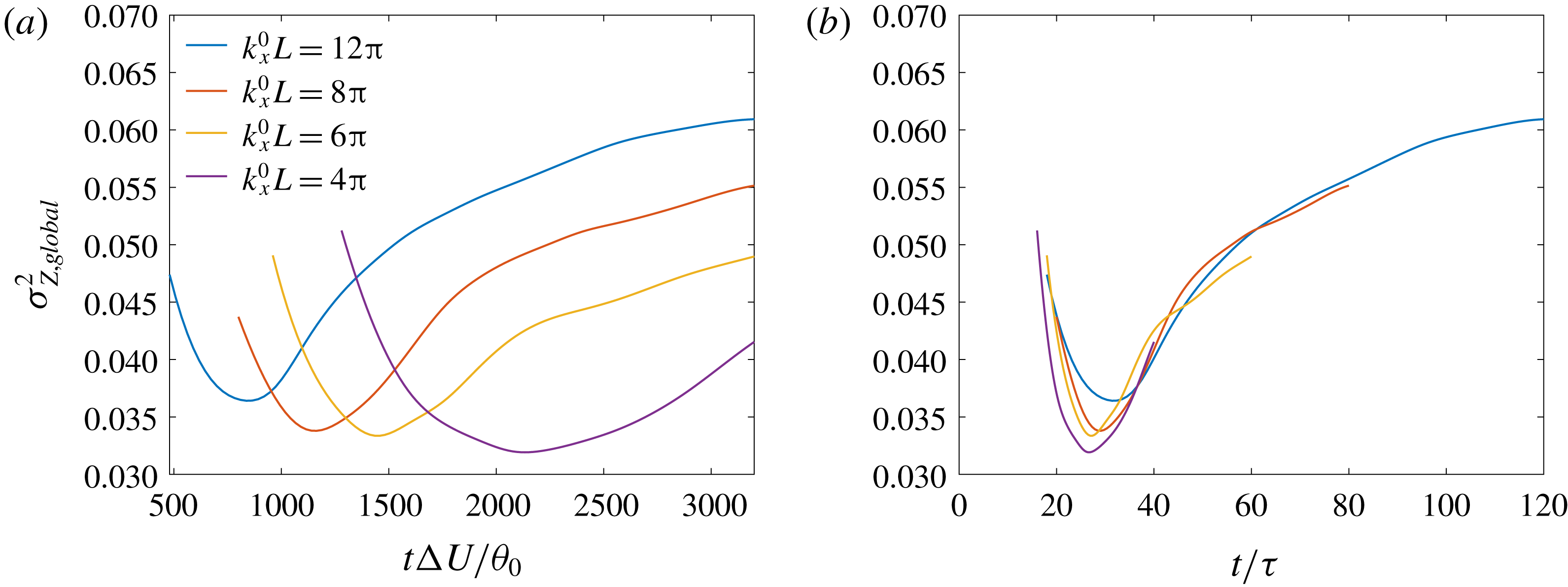
Resolved global scalar variance (3.5b
) evolution with time non-dimensionalized using (a) the initial momentum thickness,
 $\unicode[STIX]{x1D703}_{0}$
, and (b) the reciprocal of perturbation wavenumber
 $k_{x}^{0}$
as length scale. Legend is the same for both plots.

The scaled time,
 $t\unicode[STIX]{x0394}U/\unicode[STIX]{x1D703}_{0}$
, of transition from a non-marching to a marching scalar p.d.f. is governed by
 $k_{x}^{0}$
; decreasing
 $k_{x}^{0}$
delays this transition. Changes in scalar-p.d.f. character can be assessed based on the global scalar variance, given by (3.5b
) and plotted in figure 16. A marching p.d.f. with a spatially varying most probable scalar concentration has higher deviations about the global mean,
 $\unicode[STIX]{x27E6}\overline{Z}\unicode[STIX]{x27E7}\approx 1/2$
, than a non-marching p.d.f. representing a near-uniform composition. As a result, the global scalar variance (3.5b
) can exhibit a minimum that develops for each initial perturbation considered, as also observed in figures 4(a) and 5(a). The time scale
 $\unicode[STIX]{x1D70F}$
in a forced shear layer parameterizes mixing behaviour and scalar-p.d.f. character independently of other aspects of initial perturbations considered, as shown in figure 16(b).
A local minimum occurs in variance, owing to a near-uniform mixed-fluid composition or a non-marching p.d.f., at
 $t/\unicode[STIX]{x1D70F}\approx 30$
, when the flow evolves from the second to the third stage. P.d.f. transition from non-marching to marching behaviour occurs at
 $t/\unicode[STIX]{x1D70F}\approx 50$
, when the flow evolves from the third to the fourth stage, marked by a decrease in shear-layer growth and an increase in three-dimensionality of large-scale flow structures.
Resolved local scalar variance (C 6c
) from different initial conditions at (a)
 $t/\unicode[STIX]{x1D70F}\approx 6$
, (b)
 $t/\unicode[STIX]{x1D70F}\approx 18$
and (c)
 $t/\unicode[STIX]{x1D70F}\approx 40$
. Legend is the same for all plots.

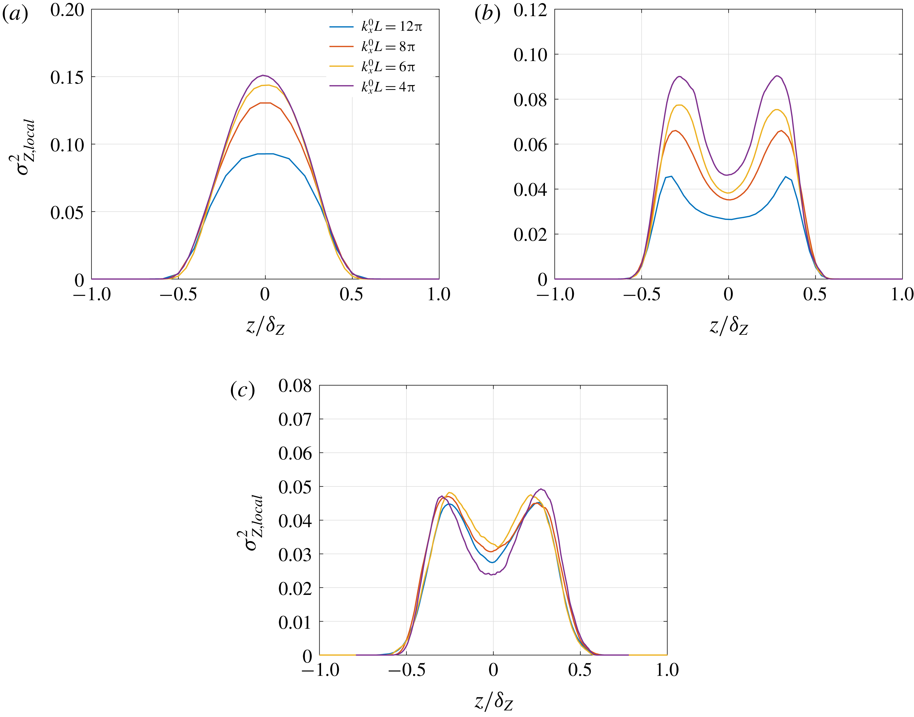
Turbulence intensity is plotted in figure 11 in terms of streamwise velocity fluctuations. The scalar-fluctuation level can be similarly assessed in the various stages of flow development in terms of the local scalar variance (C 6c ), plotted in figure 17. Similarly to the streamwise turbulence intensity, the distribution of local scalar variance evolves from that with a single peak in the first stage to that with a double peak in the second stage. However, it retains the double-peak distribution in the third stage, unlike the streamwise turbulence intensity. The local scalar-variance double-peak distribution in the third and subsequent stages is expected until pure fluid is entrained at the shear-layer boundaries. Entrainment followed by mixing at shear-layer boundaries enhances scalar fluctuations, leading to a higher local scalar variance at the boundaries, compared to the vicinity of the mid-plane where previously mixed fluid exists.
3.2.2 Effect of perturbation amplitude
Numerical simulations discussed in the previous section examine mixing layers from the initial condition in (2.3), with parameter values as specified in § 2.2 and various values of the perturbation wavenumber
 $k_{x}^{0}$
. The choice of initial perturbations leads to mixing characterized by a passive-scalar p.d.f. and variance profiles that can be scaled in terms of the time scale
 $\unicode[STIX]{x1D70F}$
(based on
 $k_{x}^{0}$
). In particular, a p.d.f. transition from non-marching to marching occurs at approximately
 $t/\unicode[STIX]{x1D70F}\approx 50$
. In this and the next section, flow sensitivity to other parameters in (2.3a–c
) is assessed for their influence on mixing and p.d.f. transition time.
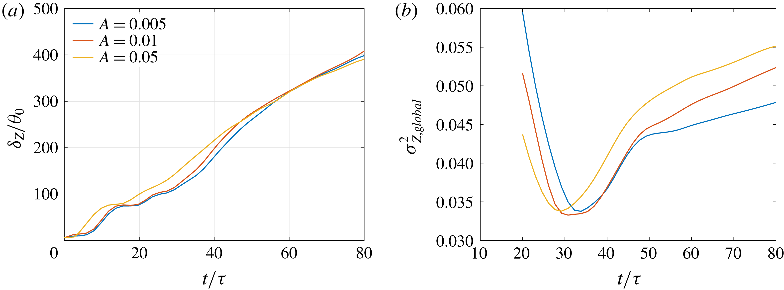
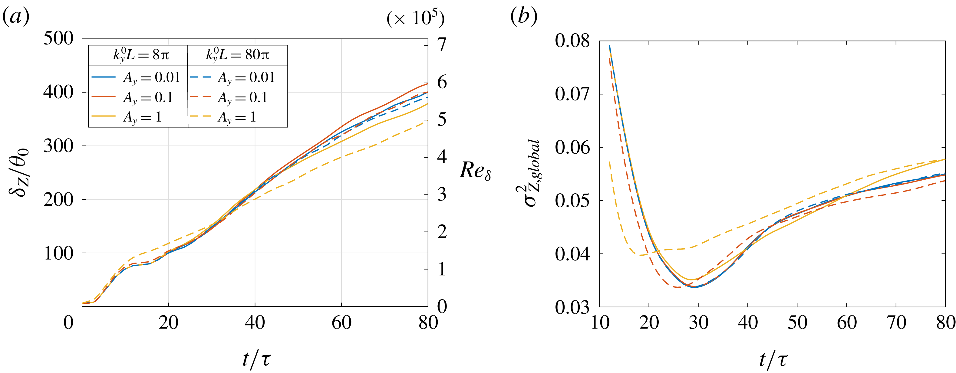
Figure 18 shows the shear-layer width based on scalar concentration and the global scalar variance simulated with three values of the perturbation amplitude
 $A$
in (2.3f
), using
 $k_{x}^{0}L=8\unicode[STIX]{x03C0}$
in (2.3) and other parameters as specified in § 2.2. The amplitude
 $A$
modulates the initial perturbation magnitude with respect to the mean profile (2.3d
). The peak velocity perturbation amplitude is varied over an order of magnitude, from approximately
 $0.75\,\%$
with
 $A=0.005$
to
 $7.5\,\%$
with
 $A=0.05$
. Turbulence intensity, calculated using
 $$\begin{eqnarray}\frac{1}{\unicode[STIX]{x0394}U}\left(\int _{-L_{x}/2}^{L_{x}/2}\int _{-L_{y}/2}^{L_{y}/2}\int _{-\unicode[STIX]{x1D6FF}_{u_{0}}/2}^{\unicode[STIX]{x1D6FF}_{u_{0}}/2}(\bar{u}^{\prime 2}+\bar{v}^{\prime 2}+\bar{w}^{\prime 2})\,\text{d}z\,\text{d}y\,\text{d}x\right)^{1/2},\end{eqnarray}$$
varies linearly from approximately
 $0.5\,\%$
with
 $A=0.005$
to
 $5\,\%$
with
 $A=0.05$
, where
 $\unicode[STIX]{x1D6FF}_{u_{0}}$
in (3.7) is the initial shear-layer width corresponding to a
 $0.01\unicode[STIX]{x0394}U$
criterion, i.e.
 $-0.49\leqslant \langle \bar{u}\rangle /\unicode[STIX]{x0394}U\leqslant 0.49$
.
As seen at early times in figure 18(a), shear-layer growth is slightly delayed with a decrease in perturbation amplitude because of the delay in initial vortex pairing. Consequently, the global scalar-variance minimum, as seen in figure 18(b), also occurs at a slightly later time with a decrease in
 $A$
. The shear layers, however, evolve through same flow stages, as described in the previous section, and the p.d.f. transition time, as seen through the change of slope in figure 18(a,b), occurs at approximately
 $t/\unicode[STIX]{x1D70F}\approx 50$
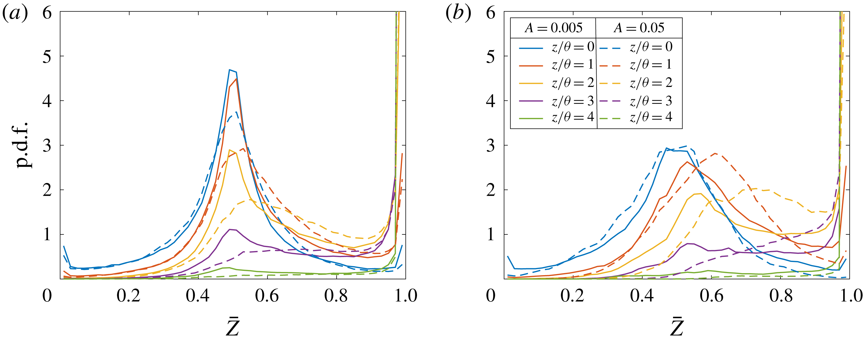
in all cases. Figure 19(a,b) confirms the p.d.f. transition time and shows the p.d.f. line plots at various cross-stream locations in the mixing layer from
 $A=0.005$
(solid lines) and
 $0.05$
(dashed lines) at
 $t/\unicode[STIX]{x1D70F}=40$
and
 $t/\unicode[STIX]{x1D70F}=60$
, respectively. The p.d.f. is seen to be non-marching at
 $t/\unicode[STIX]{x1D70F}=40$
and marching at
 $t/\unicode[STIX]{x1D70F}=60$
in both cases, despite the order-of-magnitude difference in initial perturbation magnitude.
P.d.f. peaks in figure 19(a) are higher for the low-amplitude case, as may also be inferred from a lower global variance for the low-amplitude case at
 $t/\unicode[STIX]{x1D70F}=40$
in figure 18(b), suggesting a higher probability of a mixed-fluid concentration
 $\overline{Z}=1/2$
in the low-amplitude case at
 $t/\unicode[STIX]{x1D70F}=40$
. The low variance at late times in figure 18(b) for the low-amplitude case is a result of a less small-scale mixing at the edges of the layer that produces intermediate concentrations farther from
 $\overline{Z}=1/2$
. Mixed-fluid concentrations farther from
 $\overline{Z}=1/2$
increase the global scalar variance, as also evident from (3.5b
).


Resolved-scalar p.d.f.s at various cross-stream locations from perturbation amplitude
 $A=0.005$
and
 $0.05$
in (2.3f
) with
 $k_{x}^{0}L=8\unicode[STIX]{x03C0}$
(
 $k_{x}^{0}\unicode[STIX]{x1D703}_{0}=0.025$
) in (2.3) at (a)
 $t/\unicode[STIX]{x1D70F}=40$
and (b)
 $t/\unicode[STIX]{x1D70F}=60$
. Legend is the same for both plots.

3.2.3 Effect of random noise magnitude
Random numbers,
 $g_{i}$
,
 $1\leqslant i\leqslant 3$
, are added to the initial velocity perturbations in (2.3a–c
) to facilitate shear-layer transition to turbulence. The random number magnitude with respect to perturbations’ streamwise variation is controlled by
 $A_{g}$
, which is assumed to be equal to unity in the simulations discussed in other sections;
 $A_{g}$
is varied in this section, keeping other parameters fixed, to determine its influence on mixing and p.d.f. transition.
The perturbations in (2.3a–c
) with streamwise wavenumber an order of magnitude lower than the most unstable wavenumber of the flow lead to a temporal shear-layer development analogous to the forced shear layers of Oster & Wygnanski (Reference Oster and Wygnanski1982), for which a p.d.f.-transition criterion can be estimated, as discussed in § 3.2.1. A random noise magnitude of
 $A_{g}=1$
, chosen in the simulations described in § 3.2.1, is large enough to trigger shear-layer transition to turbulence without masking the initial perturbations’ streamwise variation. A choice of
 $A_{g}\gg 1$
, with turbulence intensity kept constant by decreasing
 $A$
, overwhelms the perturbations’ streamwise variation resulting in a flow akin to unforced shear layers. On the other hand,
 $A_{g}\ll 1$
does not trigger transition to fully developed turbulent flow. Consequently, too low or too high values of
 $A_{g}$
are not considered.
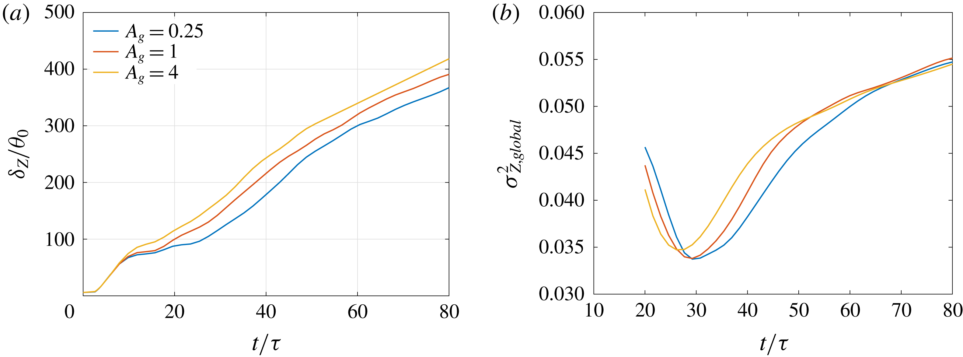
Figure 20 shows the shear-layer width based on scalar concentration and the global scalar variance with three values of
 $A_{g}$
that span an order of magnitude. Other parameters of the initial condition (2.3) are assigned values as specified in § 2.2. The turbulence intensity calculated from (3.7) varies from approximately
 $4.5\,\%$
with
 $A_{g}=0.25$
to
 $9\,\%$
with
 $A_{g}=4$
, where the increase is solely attributable to random noise, in contrast to the previous section, where the increase was attributable both to the sinusoidal forcing function and random noise.
Shear-layer growth at early times in figure 20(a) is independent of
 $A_{g}$
indicating that initial vortex pairing is unaffected by random noise and is determined by the forcing function. Between the first and the second vortex pairing, growth rates differ between cases but then remain the same for all cases, resulting in a uniform width difference after the second pairing. The global scalar-variance minimum occurs around
 $t/\unicode[STIX]{x1D70F}\approx 30$
, with the minimum for
 $A_{g}=4$
occurring slightly earlier than for
 $A_{g}=0.25$
, as also observed with the higher initial turbulence intensity cases in figure 18(b).
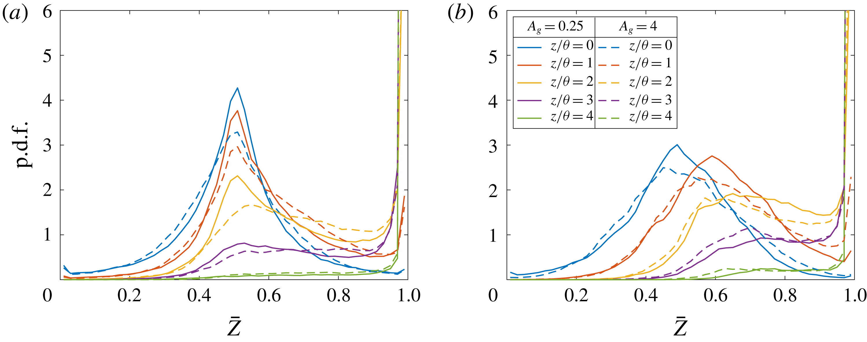
To examine the p.d.f. character, figure 21(a) and (b) show p.d.f. line plots at various cross-stream locations in the mixing layer from
 $A_{g}=0.25$
(solid lines) and
 $4$
(dashed lines) at
 $t/\unicode[STIX]{x1D70F}=40$
and
 $t/\unicode[STIX]{x1D70F}=60$
, respectively. The p.d.f. is non-marching at
 $t/\unicode[STIX]{x1D70F}=40$
and marching at
 $t/\unicode[STIX]{x1D70F}=60$
for both cases, despite an order of magnitude difference in initial random noise magnitude.
To further examine the validity of the criterion for p.d.f. transition, mixing sensitivity to initial spanwise perturbation wavenumber,
 $k_{y}^{0}$
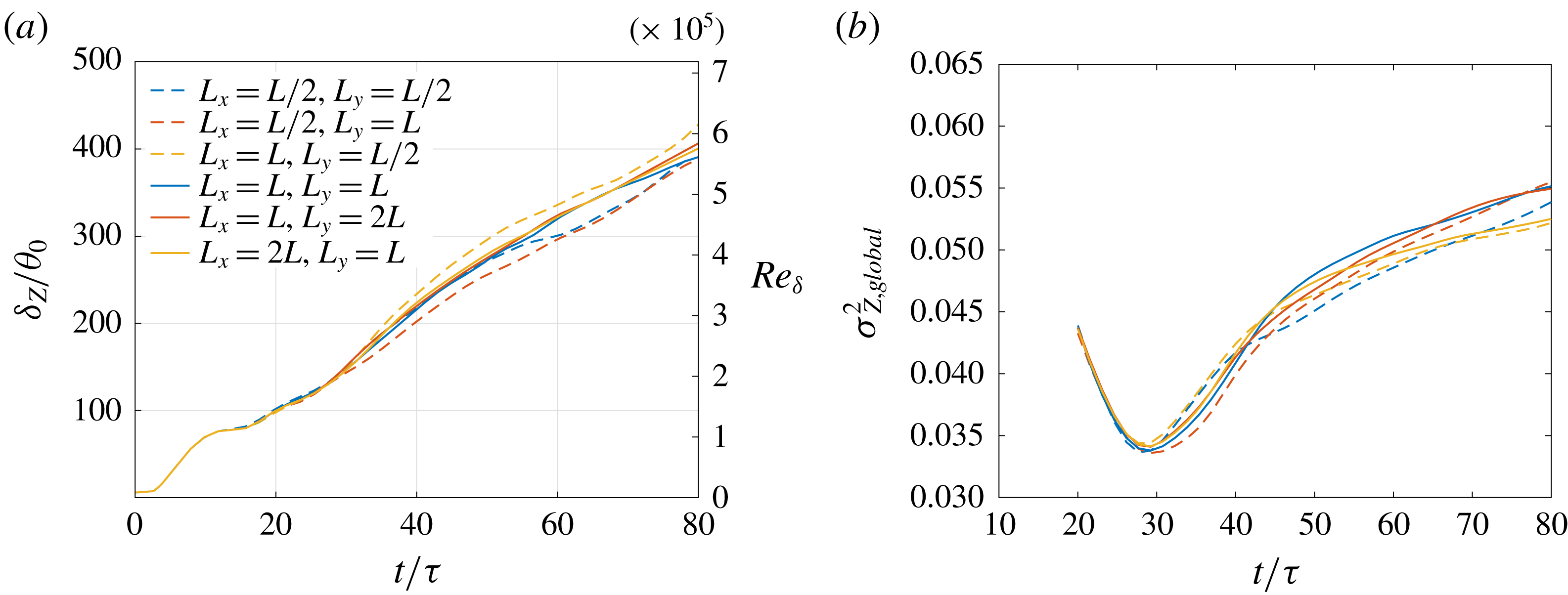
, is analysed in § B.2 and to streamwise and spanwise domain size in § C.4.


Resolved-scalar p.d.f.s at various cross-stream locations from
 $A_{g}=0.25$
and
 $4$
in (2.3a–c
) with
 $k_{x}^{0}L=8\unicode[STIX]{x03C0}$
(
 $k_{x}^{0}\unicode[STIX]{x1D703}_{0}=0.025$
) in (2.3) at (a)
 $t/\unicode[STIX]{x1D70F}=40$
and (b)
 $t/\unicode[STIX]{x1D70F}=60$
. Legend is the same for both plots.

4 Discussion
Mixed-fluid composition, characterized by a passive-scalar p.d.f., determines chemical-product formation and heat release in chemically reacting flows. Its control, through influences of flow structure can effect combustion applications ranging from automotive, to industrial, to aerospace, for example.
Shear-layer mixing is sensitive to large-scale flow structures (e.g. Rogers & Moser Reference Rogers and Moser1994; Karasso & Mungal Reference Karasso and Mungal1996; Slessor et al. Reference Slessor, Bond and Dimotakis1998; Fiscaletti et al. Reference Fiscaletti, Attili, Bisetti and Elsinga2016). Flows with organized two-dimensional structures that entrain pure fluid across the shear layer from both free streams lead to a uniform composition, or a non-marching p.d.f., whereas flows lacking organized structures exhibit a non-uniform composition or a marching p.d.f. (Rogers & Moser Reference Rogers and Moser1994). Spatial/temporal persistence of two-dimensional structures in a shear layer depends on inflow/initial perturbations. Shear layers initialized with turbulent flow develop three-dimensional structures earlier in space/time than those initialized with laminar flow (Bell & Mehta Reference Bell and Mehta1990; Slessor et al. Reference Slessor, Bond and Dimotakis1998). The scalar p.d.f. is non-marching in early regions/stages of shear-layer development and transitions to marching in the far field (in spatial flows), or at late times (in temporal flows) (e.g. Rogers & Moser Reference Rogers and Moser1994; Karasso & Mungal Reference Karasso and Mungal1996; Attili & Bisetti Reference Attili and Bisetti2012). This transition occurs earlier in flows from turbulent inflow/initial conditions than in flows from laminar conditions (Karasso & Mungal Reference Karasso and Mungal1996; Slessor et al. Reference Slessor, Bond and Dimotakis1998).
A turbulent inflow introduces a wide spectrum of disturbances, rendering a systematic study of initial perturbation effects on transition between mixing regimes and perturbation attributes that may control such transitions infeasible. A functional form of initial perturbations provides precise control of the initial condition, allowing isolation of parameters influencing mixing and p.d.f. transition. The perturbations, given by square brackets in (2.3a–c ), comprise streamwise and spanwise sinusoidal forcing functions superimposed with random noise. Parameter choices specified in § 2.2 are intended to mimic the inflow perturbations of the Oster & Wygnanski (Reference Oster and Wygnanski1982) experiments, where the forcing frequency in a spatially evolving flow can be related to the initial streamwise perturbation wavenumber of a temporal flow. Forcing frequencies an order of magnitude lower than the most amplified frequency of the flow led Oster & Wygnanski to observe inflow perturbation effects far downstream. Similarly, streamwise perturbation wavenumbers that are an order of magnitude smaller than the most amplified wavenumber influence flow and mixing characteristics until late times in a temporal flow, as shown in § 3.2.1.
Forced shear layers are characterized by nonlinear spread/growth rates in early stages, as shown in figures 2 and 9 at moderate- and high-
 $Re_{\unicode[STIX]{x1D6FF}}$
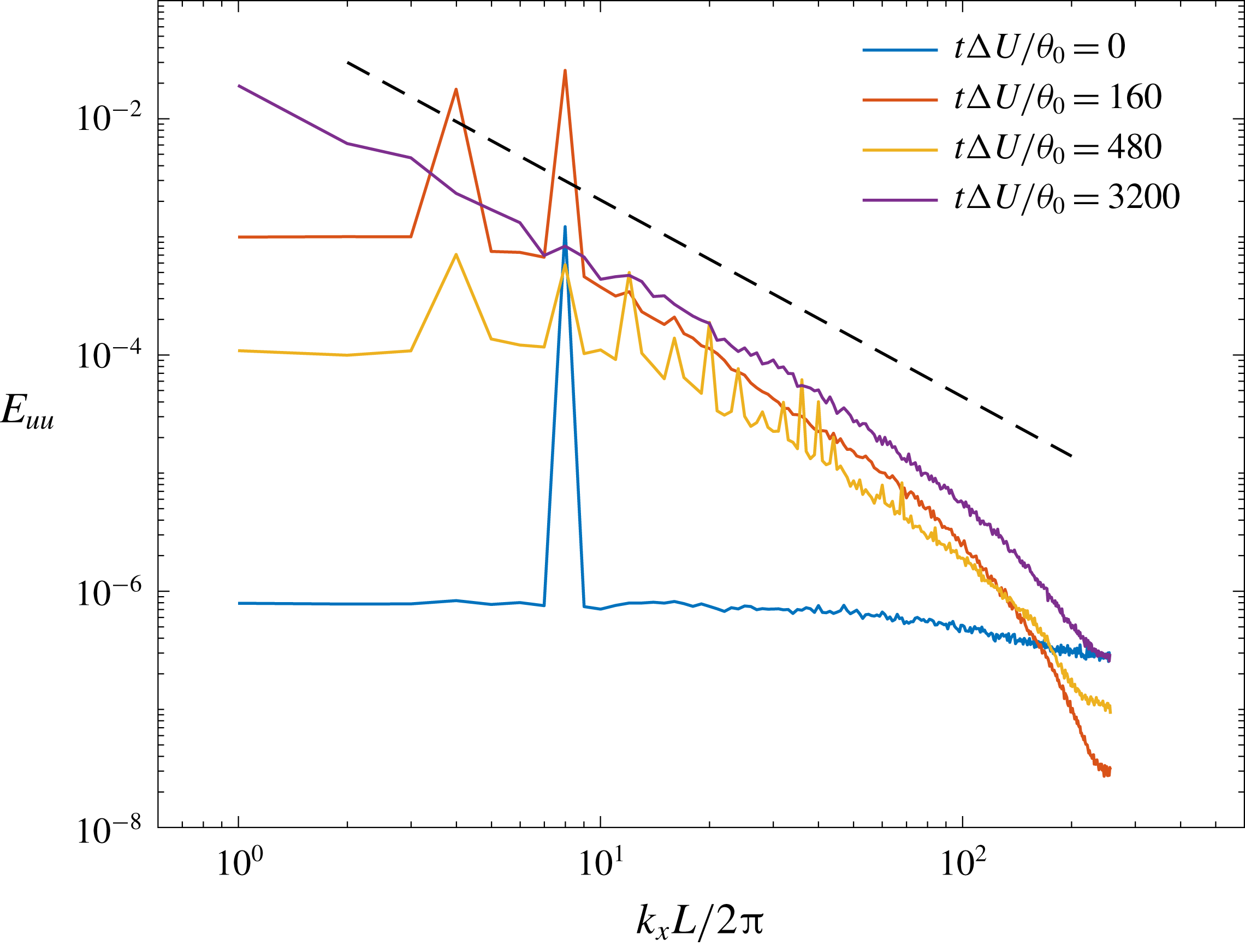
, respectively. The shear layer grows in a step-wise manner because of organized vortex mergers. Initial vortex spacing is determined by the response frequency/wavenumber of the flow to a forcing frequency/wavenumber (e.g. Ho & Huang Reference Ho and Huang1982), unlike in unforced shear layers where the most amplified frequency/wavenumber of the flow, from linear analysis, becomes the response frequency/wavenumber. To exemplify this aspect of forced shear layers, figure 22 shows the evolution of one-dimensional spectra
 $$\begin{eqnarray}E_{uu}(k_{x})=\langle |\text{DFT}_{k_{x}}(\bar{u}(x,y,z=0))|^{2}\rangle _{y}\end{eqnarray}$$
in a shear layer from the initial condition of § 2.2, with
 $k_{x}^{0}L=8\unicode[STIX]{x03C0}$
. At initial time,
 $t\unicode[STIX]{x0394}U/\unicode[STIX]{x1D703}_{0}=0$
, a peak in spectrum occurs at the forcing wavenumber
 $2k_{x}^{0}$
(note the factor of
 $2$
multiplying
 $k_{x}^{0}$
in (2.3a–c
). As the flow develops, a subharmonic of the forcing wavenumber is amplified around
 $t\unicode[STIX]{x0394}U/\unicode[STIX]{x1D703}_{0}=160$
, and harmonics appear around
 $t\unicode[STIX]{x0394}U/\unicode[STIX]{x1D703}_{0}=480$
. At late times, the flow becomes fully turbulent with more than a decade of
 $k_{x}^{-5/3}$
scaling for this flow that attains
 $Re_{\unicode[STIX]{x1D6FF}}\approx 5\times 10^{5}$
.


Figures 12–16 show that the time of p.d.f. transition can be controlled by changing the initial streamwise perturbation wavenumber, while keeping the initial momentum thickness fixed. The characteristic time scale
 $\unicode[STIX]{x1D70F}$
is seen to scale p.d.f. transition time, yielding approximately
 $t_{tr}\approx 50/(k_{x}^{0}\unicode[STIX]{x0394}U)$
, as noted in § 3.2. The scaled transition time is found to be similar for mixing layers at Reynolds numbers considered in §§ 3.1 and 3.2 that differ by an order of magnitude.
The transition time estimate of
 $t_{tr}\approx 50/(k_{0}\unicode[STIX]{x0394}U)$
yields different values for different perturbation wavenumbers, which corresponds to different Reynolds numbers,
 $Re_{\unicode[STIX]{x1D6FF}}$
, as shown in figure 9(a), confirming that increases in local Reynolds number beyond the mixing transition do not significantly influence the flow, or mixing (Dimotakis Reference Dimotakis2000). Measurements also rule out a discernible parametric dependence of the scalar p.d.f. character on
 $Re_{\unicode[STIX]{x1D6FF}}$
, as reported by Slessor et al. (Reference Slessor, Bond and Dimotakis1998).
Batt (Reference Batt1975) and later Bell & Mehta (Reference Bell and Mehta1990), among others, observed a reduction in shear-layer growth when the inflow splitter-plate boundary layer was tripped. Slessor et al. (Reference Slessor, Bond and Dimotakis1998) observed a similar reduction with tripped boundary-layer inflow in their measurements and found mixing in those flows characterized by a marching p.d.f. Reduction in shear-layer growth is also observed in the present results when the p.d.f. transitions to a marching type at
 $t/\unicode[STIX]{x1D70F}\approx 50$
, as seen in figure 9(b). P.d.f. transition is correlated with decreasing two-dimensional flow organization, leading to a reduction in scalar fluctuations.
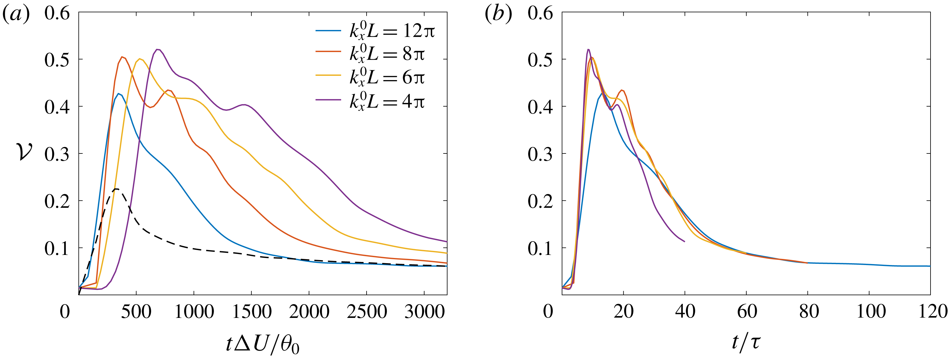
Mixing layers from laminar initial conditions superimposed with low-wavenumber disturbances or white noise, as considered in this study, exhibit significantly higher cross-stream velocity fluctuations in early stages of flow development than those initiated from turbulent initial conditions because of dominant spanwise vortex pairings in the former flow (e.g. Rogers & Moser Reference Rogers and Moser1994; Attili & Bisetti Reference Attili and Bisetti2012). The normalized integrated cross-stream turbulence intensity, defined as the non-dimensional parameter
 $$\begin{eqnarray}{\mathcal{V}}=\frac{1}{\unicode[STIX]{x1D6FF}_{\unicode[STIX]{x1D703}}}\int _{-L_{z}/4}^{L_{z}/4}\frac{\langle w^{\prime 2}\rangle }{\triangle U^{2}}\,\text{d}z,\end{eqnarray}$$
highlights differences in flow evolution to self-similarity in mixing layers from various initializations (e.g. Rogers & Moser Reference Rogers and Moser1994; Attili & Bisetti Reference Attili and Bisetti2012). Figure 23(a,b) shows the evolution of
 ${\mathcal{V}}$
from various initial perturbations considered in § 3.2.1, with respect to a non-dimensional time based on the initial momentum thickness and the initial streamwise perturbation wavelength as a length scale, respectively. Also shown in panel (a), as a dashed black line, is the profile from broadband three-dimensional initial perturbations described in § C.2. Total (resolved
 $+$
subgrid) estimate of
 $\langle w^{\prime 2}\rangle$
is obtained using (3.6).
The value of
 ${\mathcal{V}}$
peaks in the early stages, at the times of spanwise vortex pairings, and then decays to an asymptotic value as the flow approaches self-similarity. The non-dimensional times at which mixing layers from various initial perturbations reach asymptotic value is different in figure 23(a) that uses the initial momentum thickness as length scale. The profiles, however, collapse, especially at late times, if the time scale
 $\unicode[STIX]{x1D70F}$
, based on the initial streamwise perturbation wavelength as a length scale, is used, as shown in figure 23(b). The asymptotic value
 ${\sim}0.7$
reached at late times in the forced shear layers considered here is similar to values observed in the unforced shear layers of Rogers & Moser (Reference Rogers and Moser1994) and Attili & Bisetti (Reference Attili and Bisetti2012). The peak in
 ${\mathcal{V}}$
at early times from the broadband initial perturbations of § C.2 is, expectedly, lower than the peaks from the initial condition of § 2.2. Mixing layers from broadband perturbations do not develop vortical structures that span the whole (spanwise)
 $y$
-domain, resulting in local vortex pairings that generate lower cross-stream velocity fluctuations than those generated by organized spanwise vortex pairings.
Evolution of normalized integrated cross-stream turbulence intensity (4.2) plotted against time non-dimensionalized using (a) the initial momentum thickness,
 $\unicode[STIX]{x1D703}_{0}$
, and (b) the reciprocal of perturbation wavenumber
 $k_{x}^{0}$
as length scale. The dashed black line in (a) shows the profile from broadband initial perturbations described in § C.2.

The initial instability wavelength,
 $\unicode[STIX]{x1D706}$
, is a measure of the separation between the initial progression of the Kelvin–Helmholtz vortices. For forced shear layers, it is scaled by the streamwise wavelength of the initially perturbed coherent structures instead of the initial momentum thickness in unforced shear layers (Huang & Ho Reference Huang and Ho1990). With a p.d.f. transition time of
 $t_{tr}\approx 50/(k_{0}\unicode[STIX]{x0394}U)$
for the flows considered here and relating temporal shear-layer time to downstream coordinates in a spatially developing shear layer in its convective frame, the streamwise distance to p.d.f. transition may be estimated as
 $x_{tr}\simeq U_{c}t_{tr}$
, with
 $U_{c}$
the large-scale structure convection velocity (Dimotakis Reference Dimotakis1986), i.e.
 $x_{tr}\propto \unicode[STIX]{x1D706}\propto k_{0}^{-1}$
for this flow.
5 Conclusions
The present study of the evolution of mixing in a temporally developing, uniform-density, forced shear layer examined issues that were unresolved by previous experiments and numerical simulations of both spatially and temporally developing flows. In particular, some of the details of the initial/inflow conditions were found to influence both the initial stages of this flow, as well as stages from transitional to fully developed turbulence, in moderate- to high-
 $Re_{\unicode[STIX]{x1D6FF}}$
flows.
DNS and LES using the stretched-vortex, constant-coefficient Smagorinsky with various coefficient values and dynamic-Smagorinsky SGS models were performed to model turbulent shear-layer flows at moderate Reynolds numbers and to compare mixing predictions from LES using different SGS models.
Mixing in this flow can be quantified in terms of the global scalar variance; lower variance with non-marching p.d.f. implies greater mixing, while lower variance with marching p.d.f. implies less mixing. Scalar fluctuations are quantified in terms of the local scalar variance.
Flow statistics determined by large-scale structures, e.g. shear-layer width and growth, are mostly unaffected by SGS model choices. Mixed-fluid composition and scalar fluctuations, determined by small-scale processes, are sensitive to the choice. The dynamic-Smagorinsky SGS model with Lagrangian averaging provides the lowest resolved-scale mixing estimates among the three SGS models considered, while providing the best scalar-spectrum predictions when compared to unfiltered DNS results. Resolved-scale mixing estimates and scalar fluctuations from the stretched-vortex SGS model compare favourably to the box-filtered DNS results, especially at coarse grid resolutions.
The form of the filter is ambiguous in LES that does not employ an explicit filter and, therefore, agreement with box-filtered DNS results may not be indicative of SGS-model accuracy. In such cases, SGS models can be better assessed by comparisons of total (resolved + subgrid) estimates between LES and DNS. Because of its structure, the stretched-vortex SGS model provides subgrid scalar-variance and -dissipation estimates without ambiguity in their definition and without additional independent modelling that is often required with eddy-viscosity models. Total scalar variance and dissipation estimates in LES using the stretched-vortex SGS model exhibit good agreement with DNS in the turbulent-flow regime. Mean velocity and Reynolds stresses in the self-similar regime compared with experimental results further validate the numerical set-up and the LES.
The time of global scalar-variance minimum and changes in p.d.f. character are equally well predicted by all SGS models considered. As a consequence, many conclusions of this study, primarily inferred from those metrics, are independent of SGS model choice.
LES of high-
 $Re_{\unicode[STIX]{x1D6FF}}$
shear-layer flows further assess initial-condition influence on mixing. To examine flow stages with different mixing characteristics, initial perturbations mimicking two-dimensional forcing employed in experimental studies (e.g. Oster & Wygnanski Reference Oster and Wygnanski1982; Ho & Huang Reference Ho and Huang1982) are considered. The perturbations lead to shear flows with similar temporal growth behaviour as spatial growth observed experimentally in forced shear layers. The turbulence intensity distribution across the shear layer at different times also compares favourably with the distribution at corresponding stages reported for spatially developing shear layers.
Mixing, as characterized by the scalar p.d.f., evolves from non-marching to marching as the large-scale flow structures become three dimensional. Flow regimes with non-marching p.d.f. are characterized by higher scalar gradients and fluctuations than the regimes with marching p.d.f. The p.d.f. transition time can be controlled by the initial streamwise perturbation wavenumber and is not influenced by the local Reynolds number, as discussed in §§ 3.2 and 4. The transition time also remains largely unchanged by an order of magnitude variation in perturbation amplitude
 $A$
, in (2.3f
), and random noise magnitude
 $A_{g}$
, in (2.3a–c
), as shown in §§ 3.2.2 and 3.2.3, respectively.
The streamwise domain extent in a temporal shear-layer simulation can constrain the number of vortex pairings. Shear layers grow in the early stages primarily by vortex amalgamations that influence mixing and p.d.f. transition. Section C.4 shows that an increase in streamwise domain length from
 $L$
to
 $2L$
does not alter mixing estimates or the p.d.f.-transition time, based on the time scale
 $\unicode[STIX]{x1D70F}$
. An increase in spanwise domain size yielded similar conclusions, confirming that spatial domain extents in the present simulations are sufficiently large to not influence conclusions of the study.
The present study examined mixing and p.d.f. transition in forced shear layers from minimal initial spanwise perturbation variation. At low amplitudes of spanwise perturbation variation,
 $A_{y}$
, the wavenumber
 $k_{y}^{0}$
has negligible influence on shear-layer growth and p.d.f-transition time, as discussed in § B.2.
Acknowledgements
This work was supported by the Department of Energy, National Nuclear Security Administration (DOE/NNSA), Award Number DE-NA0002382, the AFOSR Grant FA9550-12-1-0461 and the John K. Northrop Chair of the California Institute of Technology, with additional computational equipment support by the NSF MRI Grant EIA-0079871 and the AFOSR DURIP Grant FA9550-10-1-0553. This research also used resources of the Argonne Leadership Computing Facility (ALCF), which is a DOE Office of Science User Facility supported under Contract DE-AC02-06CH11357. The
 $2048^{3}$
DNS and all LES described in this paper were performed on the 512-core Lykos-Skepsis GALCIT cluster developed by Dr D. Lang under DOE support. Additional support and assistance by Dr D. Lang, Dr R. Balakrishnan and the ALCF technical support staff with computational resources used in this study is gratefully acknowledged.
Appendix A. Subgrid-scale models
A.1 Stretched-vortex model
The stretched-vortex SGS model represents fine-scale turbulence in terms of vortex-based models (Pullin & Saffman Reference Pullin and Saffman1994, Reference Pullin and Saffman1998), with local unidirectional vortical structures providing the basis for the representation of subgrid dynamics in each cell (Misra & Pullin Reference Misra and Pullin1997; Pullin Reference Pullin2000). The SGS stress and scalar flux that close (2.1b ) and (2.1c ) are then given by
 $$\begin{eqnarray}\displaystyle \unicode[STIX]{x1D70F}_{ij} & = & \displaystyle (\unicode[STIX]{x1D6FF}_{ij}-e_{i}^{v}e_{j}^{v})K,\end{eqnarray}$$
 $$\begin{eqnarray}\displaystyle q_{j} & = & \displaystyle -\frac{1}{2}\unicode[STIX]{x1D6E5}_{f}K^{1/2}(\unicode[STIX]{x1D6FF}_{ij}-e_{i}^{v}e_{j}^{v})\frac{\unicode[STIX]{x2202}\overline{Z}}{\unicode[STIX]{x2202}x_{i}},\end{eqnarray}$$
 $K$
is the subgrid kinetic energy,
 $\unicode[STIX]{x1D6E5}_{f}$
is the SGS spatial filter width,
 $\unicode[STIX]{x1D6FF}_{ij}$
is the Kronecker delta and
 $e_{i}^{v}$
denotes the components of a unit vector aligned with the subgrid vortex.
Subgrid kinetic energy,
 $K$
, in (A 1a
) and (A 1b
) is given by
 $$\begin{eqnarray}K=\int _{\unicode[STIX]{x03C0}/\unicode[STIX]{x1D6E5}_{f}}^{\infty }E(k)\,\text{d}k,\end{eqnarray}$$
where
 $E(k)$
is the energy spectrum of the Lundgren spiral vortex (Pullin Reference Pullin2000),
 $$\begin{eqnarray}E(k)={\mathcal{K}}_{0}\unicode[STIX]{x1D700}^{2/3}k^{-5/3}\exp \left(-\frac{2k^{2}\unicode[STIX]{x1D708}}{3|\bar{S}_{v}|}\right).\end{eqnarray}$$
Here,
 ${\mathcal{K}}_{0}$
is the Kolmogorov prefactor,
 $\unicode[STIX]{x1D700}$
is the local cell-averaged dissipation rate and
 $$\begin{eqnarray}\bar{S}_{v}=e_{i}^{v}e_{j}^{v}\overline{\unicode[STIX]{x1D61A}}_{ij}\end{eqnarray}$$
is the strain aligned with the subgrid-vortex axis, where the resolved strain-rate tensor is
 $\overline{\unicode[STIX]{x1D61A}}_{ij}=(\unicode[STIX]{x2202}\bar{u}_{i}/\unicode[STIX]{x2202}x_{j}+\unicode[STIX]{x2202}\bar{u}_{j}/\unicode[STIX]{x2202}x_{i})/2$
. The product
 ${\mathcal{K}}_{0}\unicode[STIX]{x1D700}^{2/3}$
in (A 3) is calculated from
 $$\begin{eqnarray}{\mathcal{K}}_{0}\unicode[STIX]{x1D700}^{2/3}=\frac{\bar{F}_{2}}{A\unicode[STIX]{x1D6E5}_{f}^{2/3}},\end{eqnarray}$$
where
 $A=4\int _{\unicode[STIX]{x03C0}/\unicode[STIX]{x1D6E5}_{f}}^{\infty }x^{-5/3}(1-(\sin x/x))\,\text{d}x\approx 1.90695$
and
 $\bar{F}_{2}(\boldsymbol{x})$
is the local resolved second-order velocity structure function (Métais & Lesieur Reference Métais and Lesieur1992; Voelkl, Pullin & Chan Reference Voelkl, Pullin and Chan2000) estimated from
 $$\begin{eqnarray}\bar{F}_{2}(\boldsymbol{x})=\frac{1}{6}\mathop{\sum }_{j=1}^{3}((\unicode[STIX]{x1D6FF}\bar{u}_{1}^{+})^{2}+(\unicode[STIX]{x1D6FF}\bar{u}_{2}^{+})^{2}+(\unicode[STIX]{x1D6FF}\bar{u}_{3}^{+})^{2}+(\unicode[STIX]{x1D6FF}\bar{u}_{1}^{-})^{2}+(\unicode[STIX]{x1D6FF}\bar{u}_{2}^{-})^{2}+(\unicode[STIX]{x1D6FF}\bar{u}_{3}^{-})^{2})_{j},\end{eqnarray}$$
where
 $(\unicode[STIX]{x1D6FF}\bar{u}_{i}^{\pm })_{j}=\bar{u}_{i}(\boldsymbol{x}\pm \unicode[STIX]{x0394}x_{j})-\bar{u}_{i}(\boldsymbol{x})$
is the velocity difference of component
 $u_{i}$
in
 $j$
-direction at
 $\boldsymbol{x}$
. Subgrid vortices are assumed to align with the most extensional eigenvector of the resolved strain-rate tensor,
 $\overline{\unicode[STIX]{x1D61A}}_{ij}$
, and a SGS filter width of
 $\unicode[STIX]{x1D6E5}_{f}=\unicode[STIX]{x0394}x$
, the spatial grid spacing, is used for all simulations.
The LES code with the stretched-vortex model was successfully used in Matheou et al. (Reference Matheou, Chung, Nuijens, Stevens and Teixeira2011), Matheou & Chung (Reference Matheou and Chung2014), Matheou & Bowman (Reference Matheou and Bowman2016) and Sharan et al. (Reference Sharan, Matheou and Dimotakis2018a ).
A.2 Smagorinsky eddy-viscosity model
The SGS stress and scalar flux in a Smagorinsky-type eddy-viscosity closure (Smagorinsky Reference Smagorinsky1963; Germano et al. Reference Germano, Piomelli, Moin and Cabot1991) is given by
 $$\begin{eqnarray}\displaystyle \unicode[STIX]{x1D70F}_{ij}-\frac{1}{3}\unicode[STIX]{x1D6FF}_{ij}\unicode[STIX]{x1D70F}_{kk} & = & \displaystyle -2\unicode[STIX]{x1D708}_{T}\overline{\unicode[STIX]{x1D61A}}_{ij}=-2(C_{s}\unicode[STIX]{x1D6E5}_{f})^{2}|\overline{\unicode[STIX]{x1D64E}}|\overline{\unicode[STIX]{x1D61A}}_{ij},\end{eqnarray}$$
 $$\begin{eqnarray}\displaystyle q_{j} & = & \displaystyle -\frac{\unicode[STIX]{x1D708}_{T}}{Sc_{T}}\frac{\unicode[STIX]{x2202}\overline{Z}}{\unicode[STIX]{x2202}x_{j}},\end{eqnarray}$$
where
 $$\begin{eqnarray}\unicode[STIX]{x1D708}_{T}=(C_{s}\unicode[STIX]{x1D6E5}_{f})^{2}|\overline{\unicode[STIX]{x1D64E}}|\quad \text{and}\quad |\overline{\unicode[STIX]{x1D64E}}|\equiv (2\overline{\unicode[STIX]{x1D61A}}_{ij}\overline{\unicode[STIX]{x1D61A}}_{ij})^{1/2}.\end{eqnarray}$$
Constant as well as dynamically calculated values of the coefficients
 $C_{s}$
and
 $Sc_{T}$
are considered.
The dynamic implementation follows the Lagrangian averaging procedure of Meneveau, Lund & Cabot (Reference Meneveau, Lund and Cabot1996). The coefficient
 $C_{s}$
is obtained from
 $$\begin{eqnarray}C_{s}^{2}=\frac{\mathscr{I}_{LM}}{\mathscr{I}_{MM}},\end{eqnarray}$$
where
 $\mathscr{I}_{LM}$
and
 $\mathscr{I}_{MM}$
are the solutions to relaxation–transport equations (Meneveau et al.
Reference Meneveau, Lund and Cabot1996, (3.8) and (3.9)). The method described in (Meneveau et al.
Reference Meneveau, Lund and Cabot1996, § 3.3), with trilinear interpolation, is used to advance the transport equations. The resolved turbulent stress,
 $L_{ij}$
, and its Smagorinsky model estimate,
 $M_{ij}$
, that comprise the solution of
 $\mathscr{I}_{LM}$
and
 $\mathscr{I}_{MM}$
are defined as
 $$\begin{eqnarray}L_{ij}=\widehat{\bar{u}_{i}\bar{u}_{j}}-\widehat{\bar{u}}_{i}\widehat{\bar{u}}_{j},\quad M_{ij}=2\unicode[STIX]{x1D6E5}_{f}^{2}[\widehat{|\overline{\unicode[STIX]{x1D64E}}|\overline{\unicode[STIX]{x1D61A}}_{ij}}-4|\widehat{\overline{\unicode[STIX]{x1D64E}}}|\widehat{\overline{\unicode[STIX]{x1D61A}}}_{ij}],\end{eqnarray}$$
where the overbar,
 $\bar{\cdot }$
, denotes filtering at scale
 $\unicode[STIX]{x1D6E5}_{f}$
and the overhat,
 $\widehat{\cdot }$
, denotes filtering at scale
 $2\unicode[STIX]{x1D6E5}_{f}$
.
A similar procedure is followed to obtain the turbulent Schmidt number,
 $Sc_{T}$
, given by
 $$\begin{eqnarray}Sc_{T}=C_{s}^{2}\frac{\mathscr{I}_{MM}^{(Z)}}{\mathscr{I}_{LM}^{(Z)}},\end{eqnarray}$$
where the scalar fluxes,
 $L_{j}^{(Z)}$
, and their Smagorinsky model estimates,
 $M_{j}^{(Z)}$
, required to solve for
 $\mathscr{I}_{LM}^{(Z)}$
and
 $\mathscr{I}_{MM}^{(Z)}$
are defined as (e.g. Lilly Reference Lilly1992)
 $$\begin{eqnarray}L_{j}^{(Z)}=\widehat{\bar{Z}\bar{u}_{j}}-\widehat{\bar{Z}}\widehat{\bar{u}}_{j},\quad M_{j}^{(Z)}=2\unicode[STIX]{x1D6E5}_{f}^{2}\left[\widehat{|\overline{\unicode[STIX]{x1D64E}}|\frac{\unicode[STIX]{x2202}\bar{Z}}{\unicode[STIX]{x2202}x_{j}}}-4|\widehat{\overline{\unicode[STIX]{x1D64E}}}|\widehat{\frac{\unicode[STIX]{x2202}\bar{Z}}{\unicode[STIX]{x2202}x_{j}}}\right].\end{eqnarray}$$
A SGS filter width of
 $\unicode[STIX]{x1D6E5}_{f}=\unicode[STIX]{x0394}x$
, the spatial grid spacing, is used for all simulations.
The constant-coefficient Smagorinsky SGS model implementation was used in Matheou et al. (Reference Matheou, Chung, Nuijens, Stevens and Teixeira2011) and Matheou & Dimotakis (Reference Matheou and Dimotakis2016). The dynamic-Smagorinsky SGS implementation described above was tested and validated in, e.g. Sharan (Reference Sharan2016) and Sharan, Pantano & Bodony (Reference Sharan, Pantano and Bodony2018b ).
Appendix B. Initial condition
B.1 Divergence-free velocity
The simulations discussed in § 3 are initialized with velocity components (2.3a–c ) projected onto a solenoidal basis, using (2.2). Since the goal of the study is to examine forced perturbations’ influence on mixing-layer characteristics, it is important to ensure that the projection does not alter the intended disturbance profile.
Figure 24(a) shows the initial streamwise velocity (2.3a
) along the line
 $y=z=0$
for
 $k_{x}^{0}L=8\unicode[STIX]{x03C0}$
(in blue) and the velocity profile after imposing the divergence-free condition (in red). To examine the wavenumber character of velocity disturbances, figure 24(b) shows the one-dimensional spectra on the mixing-layer mid-plane calculated from
 $$\begin{eqnarray}\hat{u} (k_{x})=\langle |\text{DFT}_{k_{x}}(u(x,y,z=0))|\rangle _{y}.\end{eqnarray}$$
The spike in amplitude in figure 24(b) occurs at the forcing wavenumber
 $2k_{x}^{0}$
, see (2.3a–c
). As evident from the figure, the application of the divergence-free condition marginally reduces the amplitude at
 $2k_{x}^{0}$
and at large wavenumbers. However, the forcing wavenumber, where the spike in amplitude occurs, crucial to this study, remains unchanged. Similar behaviour was observed with other values of
 $k_{x}^{0}$
in (2.3) and in the one-dimensional spectrum in the spanwise direction to evaluate the effect on spanwise forcing, which ensures that the forcing wavelength in each direction is preserved after application of the divergence-free condition to the velocity field (2.3a–c
).
Initial (a) streamwise velocity,
 $u$
, at
 $y\,=\,0$
and
 $z\,=\,0$
, (b) streamwise-velocity one-dimensional spectra on the mixing-layer mid-plane (B 1) before (labelled ‘Non-solenoidal’) and after (labelled ‘Solenoidal’) imposing the divergence-free condition. Legend is the same for both plots.

B.2 Effect of spanwise forcing
The initial condition (2.3) with parameters as specified in § 2.2 mimics forcing in the experiments of Oster & Wygnanski (Reference Oster and Wygnanski1982), as described in § 3.2.1. The inflow/initial perturbations’ spanwise variation in those experiments are small and, therefore, a small value of
 $A_{y}$
(
 $=0.01$
) is employed for simulations described in rest of the paper. In this appendix, we examine the effect of the perturbation spanwise wavenumber,
 $k_{y}^{0}$
, on mixing and p.d.f. transition with small as well as large values of amplitude
 $A_{y}$
.
Evolution of (a) shear-layer width (1.1b
) and (b) resolved global scalar variance (3.5b
) in LES using the stretched-vortex SGS model with various perturbation spanwise wavenumber,
 $k_{y}^{0}$
, and
 $k_{x}^{0}L=8\unicode[STIX]{x03C0}$
(
 $k_{x}^{0}\unicode[STIX]{x1D703}_{0}=0.025$
) in (2.3). Other parameters in (2.3) are as specified in § 2.2, including,
 $A_{y}=0.01$
.

Evolution of (a) shear-layer width (1.1b
) and (b) resolved global scalar variance (3.5b
) in LES using the stretched-vortex SGS model with various
 $A_{y}$
and
 $k_{y}^{0}$
, using
 $k_{x}^{0}L=8\unicode[STIX]{x03C0}$
(
 $k_{x}^{0}\unicode[STIX]{x1D703}_{0}=0.025$
) in (2.3). Legend is the same for both plots.

Resolved-scalar p.d.f. at various cross-stream locations using
 $A_{y}=0.01$
and
 $1$
with
 $k_{y}^{0}L=8\unicode[STIX]{x03C0}$
(
 $k_{y}^{0}\unicode[STIX]{x1D703}_{0}=0.025$
) and
 $k_{x}^{0}L=8\unicode[STIX]{x03C0}$
(
 $k_{x}^{0}\unicode[STIX]{x1D703}_{0}=0.025$
) in (2.3) at (a)
 $t/\unicode[STIX]{x1D70F}=40$
and (b)
 $t/\unicode[STIX]{x1D70F}=60$
. Legend is the same for both plots.

Figure 25 shows the shear-layer width based on the scalar concentration and the global scalar variance with the initial condition (2.3), using various values of the spanwise perturbation wavenumber,
 $k_{y}^{0}$
, with
 $k_{x}^{0}L=8\unicode[STIX]{x03C0}$
, and other parameters as specified in § 2.2. As evident from figure 25, changes in spanwise wavenumber by an order of magnitude do not influence shear-layer growth, or mixed-fluid composition, except marginally at late times. The p.d.f. character and transition time also remain unchanged by variation of
 $k_{y}^{0}$
at a small value of
 $A_{y}=0.01$
.
Values of
 $A_{y}\sim 1$
in (2.3a
)–(2.3c
) introduce perturbations that vary in spanwise direction as much as in the streamwise direction. Such initializations may differ from the forced mixing-layer experiments of Oster & Wygnanski (Reference Oster and Wygnanski1982), where the rigid flap used for forcing has a uniform shape/thickness along the span, introducing disturbances that vary minimally in spanwise direction.
To examine the effect of increasing
 $A_{y}$
, figure 26 shows the shear-layer width based on scalar concentration and global scalar variance in shear layers with
 $A_{y}=0.01$
,
 $0.1$
and
 $1$
, and initial spanwise perturbation wavenumbers
 $k_{y}^{0}L=8\unicode[STIX]{x03C0}$
(solid lines) and
 $k_{y}^{0}L=80\unicode[STIX]{x03C0}$
(dashed lines). A streamwise wavenumber of
 $k_{x}^{0}L=8\unicode[STIX]{x03C0}$
is used with other parameters in (2.3), as specified in § 2.2.
 $k_{y}^{0}L=80\unicode[STIX]{x03C0}$
(
 $k_{y}^{0}\unicode[STIX]{x1D703}_{0}=0.25$
) is of the same order as the most unstable wavenumber (see § 2.2).
For
 $k_{y}^{0}L=8\unicode[STIX]{x03C0}$
, an increase in
 $A_{y}$
results in noticeable shear-layer growth differences at late times, as shown in figure 26(a). Similar behaviour is observed for
 $k_{y}^{0}L=80\unicode[STIX]{x03C0}$
with differences more pronounced and appearing much earlier in time for
 $A_{y}=1$
. Mixed-fluid composition, inferred from figure 26(b), shows minor differences with increasing
 $A_{y}$
for
 $k_{y}^{0}L=8\unicode[STIX]{x03C0}$
, shown in solid lines. A global scalar-variance minimum occurs around the same non-dimensional time,
 $t/\unicode[STIX]{x1D70F}\approx 30$
. P.d.f. transition, as shown in the p.d.f. lineplots at
 $t/\unicode[STIX]{x1D70F}=40$
and
 $60$
in figure 27, occurs at approximately
 $t/\unicode[STIX]{x1D70F}\approx 50$
for amplitudes
 $A_{y}$
that vary over two orders of magnitude. P.d.f. profiles for
 $A_{y}=0.01$
(solid lines) and 1 (dashed lines) in figure 27 match fairly well with each other indicating that the magnitude of perturbations’ spanwise variation, when its wavelength is an order of magnitude larger than the wavelength of the most unstable mode, has minimal influence on mixing.
For
 $k_{y}^{0}L=80\unicode[STIX]{x03C0}$
, an increase in
 $A_{y}$
yields larger shear-layer growth and variance differences, especially for
 $A_{y}=1$
, as shown in figure 26. A global scalar-variance minimum occurs early in time with increase in
 $A_{y}$
, as seen from figure 26(b). P.d.f. transition, as observed in the p.d.f. lineplots at
 $t/\unicode[STIX]{x1D70F}=40$
and
 $60$
in figure 28, occurs around
 $t/\unicode[STIX]{x1D70F}\approx 50$
for
 $A_{y}=0.01$
, but at an early time for
 $A_{y}=1$
, as inferred from the dashed lines in figure 28(a) which exhibit a marching behaviour at
 $t/\unicode[STIX]{x1D70F}=40$
.
The present study focuses on forced shear layers from initial perturbations with minimal spanwise variation, analogous to the experiments of Oster & Wygnanski (Reference Oster and Wygnanski1982). A detailed discussion of mixing characteristics in shear layers from perturbations with significant spanwise variation at wavenumbers around the most unstable mode is beyond the scope of this study.
An increase in
 $A_{y}$
, with a fixed amplitude
 $A$
in (2.3f
), as considered in the results shown in this section, increases the initial turbulence intensity calculated from (3.7). Simulations using values of
 $A$
adjusted to preserve turbulence intensity with an increase in
 $A_{y}$
yielded similar results (not shown here for brevity), for various
 $k_{y}^{0}$
and
 $A_{y}$
, suggesting that the initial turbulence intensity has minimal influence on the mixing (p.d.f.) character, as also observed in §§ 3.2.2 and 3.2.3.
Resolved-scalar p.d.f. at various cross-stream locations using
 $A_{y}=0.01$
and
 $1$
with
 $k_{y}^{0}L=80\unicode[STIX]{x03C0}$
(
 $k_{y}^{0}\unicode[STIX]{x1D703}_{0}=0.25$
) and
 $k_{x}^{0}L=8\unicode[STIX]{x03C0}$
(
 $k_{x}^{0}\unicode[STIX]{x1D703}_{0}=0.025$
) in (2.3) at (a)
 $t/\unicode[STIX]{x1D70F}=40$
and (b)
 $t/\unicode[STIX]{x1D70F}=60$
. Legend is the same for both plots.

Appendix C. Simulation validation
C.1 Filtered DNS solution

Assessment of SGS-model performance by comparisons of LES results against DNS results is complicated by the interplay between numerical discretization and SGS-model errors. Moreover, the functional form of initial profiles that are smoothly resolved on a DNS mesh may not be adequately resolved on a LES grid with significantly fewer points, further compromising one-to-one comparisons. To mitigate these errors, filtered DNS solutions are typically used to initialize LES and for LES validation. However, it is difficult to ascertain the exact form and effect of the filter in LES that do not employ an explicit filter. Sharp cutoff spectral and box filters are generally used in such cases for analyses.
One-dimensional spectra along the streamwise direction on the mixing-layer mid-plane at
 $t/\unicode[STIX]{x1D70F}=80$
from DNS and filtered DNS using sharp cutoff spectral and box filter. (a) Scalar spectra
 $E_{ZZ}(k_{x})$
(3.3); (b) streamwise scalar-gradient spectra
 $k_{x}^{2}E_{ZZ}(k_{x})$
.

To examine the behaviour of those filters with respect to scalar mixing and fluctuations, figure 29 compares the global and local scalar variance between the sharp cutoff spectrally filtered and box-filtered DNS solutions. Spectrally filtered results are denoted by ‘Spectral-filt DNS’ whereas box-filtered results by ‘Box-filt DNS’. Spectrally filtered results are similar to those from unfiltered DNS, while the box filter is more diffusive leading to higher global and lower local scalar variance. One-dimensional mid-plane scalar spectra of the filtered solutions are shown in figure 30, which highlights the dissipation introduced by the box filter.
C.2 Mixing layer from broadband initial perturbations
Mixing layers that develop from turbulent inflow conditions, obtained by tripping the boundary layers on the splitter plate, attain self-similarity at shorter axial distances than those from untripped (laminar) inflow in spatially evolving shear flows (Bell & Mehta Reference Bell and Mehta1990; Karasso & Mungal Reference Karasso and Mungal1996). Likewise, in computational studies of temporally evolving flows, mixing layers from three-dimensional (pseudo-)turbulent initial disturbances reach self-similarity sooner than flows initialized with dominant two-dimensional or random disturbances (Rogers & Moser Reference Rogers and Moser1994; Balaras et al. Reference Balaras, Piomelli and Wallace2001).
For a validation of the present numerical simulations, flow statistics in the self-similar regime are compared against the Bell & Mehta (Reference Bell and Mehta1990) experimental results, as also performed by Rogers & Moser (Reference Rogers and Moser1994) and Pantano & Sarkar (Reference Pantano and Sarkar2002), for example. LES using the stretched-vortex SGS model of shear flow attaining
 $Re_{\unicode[STIX]{x1D703}}\approx 6500$
, comparable to
 $Re_{\unicode[STIX]{x1D703}}$
of Bell & Mehta study, are performed using
 $N=512$
. To accelerate flow evolution to self-similarity, three-dimensional disturbances with an isotropic turbulence spectrum of the form, as also used by Pantano & Sarkar (Reference Pantano and Sarkar2002),
 $$\begin{eqnarray}E(k)=\left(\frac{k}{k_{p}}\right)^{4}\exp \left[-2\left(\frac{k}{k_{p}}\right)^{2}\right],\end{eqnarray}$$
are added to the mean velocity (2.3d
), where
 $k$
is the wavenumber and
 $k_{p}$
is the peak wavenumber, chosen as
 $2\unicode[STIX]{x1D6FC}$
.
 $\unicode[STIX]{x1D6FC}$
denotes the wavenumber of the most unstable mode (see § 2.2). The initial turbulence intensity is set to 5 %.
Figure 31 shows the growth of momentum thickness with time. A solid line indicates a growth rate (3.2) of 0.015, which agrees well with the value of 0.014 observed by Rogers & Moser (Reference Rogers and Moser1994) and 0.016 obtained from the Bell & Mehta (Reference Bell and Mehta1990) results. A comparison with the momentum thickness profile of figure 2(b) from the initial condition in (2.3) shows that a mixing layer from three-dimensional initial perturbations with a spectrum (C 1) attains self-similarity earlier, as expected.
Figure 32 shows the mean streamwise velocity profile in similarity coordinates,
 $z/\unicode[STIX]{x1D703}$
, at three times during the self-similar regime. For comparison, the markers show Bell & Mehta experimental results at three axial distances of their mixing layer from tripped turbulent splitter-plate boundary layers. The LES self-similar profile shows good agreement with the Bell & Mehta profile. Figure 33 compares the Reynolds stress components in similarity coordinates. The Reynolds stresses from the LES are estimated by (3.6). The collapse of Reynolds stress profiles at various times indicates self-similarity and good agreement of the profiles with experimental data lends credence to LES accuracy.


Mean streamwise velocity in similarity coordinates from LES compared against the experimental result of Bell & Mehta (Reference Bell and Mehta1990).

Components of the Reynolds stress tensor in similarity coordinates compared against the experimental result of Bell & Mehta (Reference Bell and Mehta1990). Legend same as in figure 32.

C.3 Top and bottom wall boundary condition
A cross-stream domain length of
 $L_{z}=L$
and periodic boundaries are used for the simulations and results discussed in § 3. To ascertain that the conclusions of this study are independent of top and bottom wall influence, mixing statistics are compared in this appendix from simulations with
 $L_{z}=L/2$
,
 $L$
, and
 $2L$
, and from the application of periodic as well as slip top and bottom wall boundary conditions.
Computations with slip top and bottom walls have only a mid-plane shear layer evolving in time instead of the infinite vertical stack of layers with periodic top and bottom walls. The initial velocity (2.3a–c ) is, therefore, modified for slip-wall simulations. In particular, the mean profile is given by
 $$\begin{eqnarray}\frac{f(z)}{\unicode[STIX]{x0394}U}=\frac{1}{2}\tanh \left(\frac{z}{2\unicode[STIX]{x1D703}_{0}}\right),\end{eqnarray}$$
with
 $$\begin{eqnarray}\frac{a(z)}{\unicode[STIX]{x0394}U}=0.05\exp \left(-\frac{z^{2}}{\unicode[STIX]{x1D703}_{0}}\right).\end{eqnarray}$$


Figure 34 shows the shear-layer width and global scalar variance at different times using various cross-stream domain lengths with slip walls, and using the periodic configuration with
 $L_{z}=L$
. All results are from shear-layer LES attaining
 $Re_{\unicode[STIX]{x1D6FF}}\approx 5\times 10^{5}$
and
 $Re_{\unicode[STIX]{x1D703}}\approx 7.5\times 10^{4}$
using the stretched-vortex SGS model with
 $N=256$
and an initial condition as described in § 2.2, with a mean streamwise-velocity profile (2.3d
), an amplitude function (2.3f
) replaced by (C 2a
) and (C 2b
), respectively, and
 $k_{x}^{0}L=8\unicode[STIX]{x03C0}$
. Results from
 $L_{z}=L$
and
 $2L$
agree well with each other throughout the simulation, justifying the choice of
 $L_{z}=L$
in this study.
Evolution of (a) shear-layer width (1.1b
) and (b) resolved global scalar variance (3.5b
) in LES using the stretched-vortex SGS model with various streamwise and spanwise domain lengths using
 $k_{x}^{0}L=8\unicode[STIX]{x03C0}$
(
 $k_{x}^{0}\unicode[STIX]{x1D703}_{0}=0.025$
) in (2.3). Legend is the same for both plots.

C.4 Streamwise and spanwise domain size
Influences of computational domain size on coherent structures and flow statistics in temporal shear layers were reported by Balaras et al. (Reference Balaras, Piomelli and Wallace2001) and Mattner (Reference Mattner2011), for example. They observed that smaller domain promotes two-dimensional spanwise rollers in the late stages of the flow, resulting in different shear-layer growth and Reynolds stresses. In this appendix, the effect of streamwise and spanwise domain extent on mixing and p.d.f. transition is assessed.
Figure 35 shows the shear-layer width based on the scalar-concentration profile width and the global scalar variance from LES employing various streamwise (
 $L_{x}$
) and spanwise (
 $L_{y}$
) domain extent. Solid lines in the figure show simulation results from twice the domain size in streamwise and spanwise direction with respect to dashed line of same colour. Cross-stream domain length (
 $L_{z}$
) is fixed to
 $L$
and the initial-condition parameters as specified in § 2.2 with
 $k_{x}^{0}L=8\unicode[STIX]{x03C0}$
are used for all cases. Grid spacing in each direction is preserved when domain sizes are changed.
Shear-layer growth at early times, as evident from figure 35(a), is unaffected by changes in domain size. Differences appear only after
 $t/\unicode[STIX]{x1D70F}\approx 30$
, around the global scalar-variance minimum in figure 35(b). An increase in the streamwise or spanwise domain length from
 $L$
to
 $2L$
has a minimal influence on shear-layer growth, as seen in the solid lines in figure 35(a). A decrease in domain length from
 $L$
to
 $L/2$
, on the other hand, yields noticeable differences. A smaller streamwise domain decreases shear-layer growth in the third stage of the flow (see § 3.2.1), whereas a smaller spanwise domain increases growth. Reducing both the streamwise and spanwise domain lengths from
 $L$
to
 $L/2$
results in a negligible difference until after
 $t/\unicode[STIX]{x1D70F}\approx 50$
, when shear-layer width and growth match results from the smaller domain simulation (
 $L_{x}=L/2,$
 $L_{y}=L$
). This indicates that differences at late times from decreases in both streamwise and spanwise domain sizes are largely attributable to the streamwise domain extent, which determines the number of vortex pairings in the numerical simulation. A streamwise domain length of
 $L_{x}=L/2$
allows four initial spanwise rollers, as inferred from figure 13 for
 $L_{x}=L$
. For the time extent of the present simulations,
 $L_{x}=L/2$
hinders flow development after the second vortex pairing. However, based on the comparison with
 $L_{x}=2L$
results in figure 35(a),
 $L_{x}=L$
is sufficiently large to allow flow development without domain-size influence over times spanned in these simulations.
Mixed-fluid composition, inferred from figure 35(b), evolves through the same flow stages for all domain sizes, where the passive-scalar p.d.f. is non-marching, with a minimum variance at
 $t/\unicode[STIX]{x1D70F}\approx 30$
, and transitions to marching around
 $t/\unicode[STIX]{x1D70F}\approx 50$
. To confirm the p.d.f.-transition time, figures 36(a) and (b) show p.d.f. line plots at various cross-stream locations in the mixing layer at
 $t/\unicode[STIX]{x1D70F}=40$
and
 $60$
, respectively, from LES using streamwise domain lengths of
 $L/2$
,
 $L$
and
 $2L$
, and spanwise and cross-stream domain lengths of
 $L$
. The p.d.f. is non-marching at
 $t/\unicode[STIX]{x1D70F}=40$
and marching at
 $t/\unicode[STIX]{x1D70F}=60$
in all cases. Similar results were obtained by varying the spanwise domain length, thus, confirming that p.d.f.-transition time remains approximately the same with changes in domain length.
Resolved-scalar p.d.f. at various cross-stream locations using different streamwise domain lengths (
 $L_{x}$
) and
 $L_{y}=L_{z}=L$
with
 $k_{x}^{0}L=8\unicode[STIX]{x03C0}$
(
 $k_{x}^{0}\unicode[STIX]{x1D703}_{0}=0.025$
) in (2.3) at (a)
 $t/\unicode[STIX]{x1D70F}=40$
and (b)
 $t/\unicode[STIX]{x1D70F}=60$
. Legend is the same for both plots.

C.5 Total scalar variance and dissipation from LES using the stretched-vortex model
The structure of the stretched-vortex SGS model allows estimation of subgrid contributions to scalar variance and dissipation (e.g. Pullin & Lundgren Reference Pullin and Lundgren2001; Hill, Pantano & Pullin Reference Hill, Pantano and Pullin2006; Mattner Reference Mattner2011). The SGS scalar variance,
 $\unicode[STIX]{x1D70E}_{Z,sub}^{2}$
, in the stretched-vortex model can be estimated from (e.g. Hill et al.
Reference Hill, Pantano and Pullin2006; Mattner Reference Mattner2011)
 $$\begin{eqnarray}\unicode[STIX]{x1D70E}_{Z,sub}^{2}=2\int _{\unicode[STIX]{x03C0}/\unicode[STIX]{x1D6E5}_{f}}^{\infty }E^{(Z)}(k)\,\text{d}k,\end{eqnarray}$$
where
 $E^{(Z)}(k)$
denotes the scalar spectrum.
For the evolution of a passive scalar mixed inside a stretched-spiral vortex of a given cell, the scalar spectrum, derived in Pullin & Lundgren (Reference Pullin and Lundgren2001), is given by
 $$\begin{eqnarray}E^{(Z)}(k)=K^{(Z)}\left\{k^{-5/3}\exp \left[-\frac{(4\unicode[STIX]{x1D708}+2{\mathcal{D}})k^{2}}{3|\bar{S}_{v}|}\right]+\frac{8}{5\unicode[STIX]{x03C0}}\left(\frac{\unicode[STIX]{x1D6E4}}{\unicode[STIX]{x03C0}|\bar{S}_{v}|}\right)^{1/3}k^{-1}\exp \left(-\frac{2{\mathcal{D}}k^{2}}{3|\bar{S}_{v}|}\right)\right\},\end{eqnarray}$$
where
 $\bar{S}_{v}=e_{i}^{v}e_{j}^{v}\overline{\unicode[STIX]{x1D61A}}_{ij}$
is the strain-rate magnitude aligned with the subgrid-vortex axis, and
 $\unicode[STIX]{x1D6E4}$
denotes the subgrid-vortex circulation that determines the relative magnitude of the
 $k^{-1}$
Batchelor (Reference Batchelor1959) scalar spectrum and the
 $k^{-5/3}$
Oboukhov (Reference Oboukhov1949)-Corrsin (Reference Corrsin1951) scalar-spectrum components (C 4) in the inertial range. The value of
 $\unicode[STIX]{x1D6E4}=1000\unicode[STIX]{x1D708}$
recommended in Pullin & Lundgren (Reference Pullin and Lundgren2001) and Hill et al. (Reference Hill, Pantano and Pullin2006) for the subgrid continuation of the scalar spectrum is adopted. The prefactor
 $K^{(Z)}$
is calculated from the local spherically averaged second-order scalar structure function
 $\overline{F_{2}^{(Z)}}$
, where
 $$\begin{eqnarray}K^{(Z)}=\frac{\overline{F_{2}^{(Z)}}}{A\unicode[STIX]{x1D6E5}_{f}^{2/3}+B(\unicode[STIX]{x1D708}/|\bar{S}_{v}|)^{1/3}},\quad \overline{F_{2}^{(Z)}}=\frac{1}{6}\mathop{\sum }_{j=1}^{3}[(\unicode[STIX]{x1D6FF}\overline{Z}^{+})^{2}+(\unicode[STIX]{x1D6FF}\overline{Z}^{-})^{2}]_{j},\end{eqnarray}$$
with
 $$\begin{eqnarray}(\unicode[STIX]{x1D6FF}\overline{Z}^{\pm })_{j}=\overline{Z}(\boldsymbol{x}\pm \unicode[STIX]{x0394}x_{j})-\overline{Z}(\boldsymbol{x})\end{eqnarray}$$
the scalar difference at
 $\boldsymbol{x}$
in the
 $x_{j}$
-direction,
 $$\begin{eqnarray}A=4\int _{0}^{\unicode[STIX]{x03C0}}s^{-5/3}\left(1-\frac{\sin s}{s}\right)\,\text{d}s\approx 1.90695,\end{eqnarray}$$
and
 $$\begin{eqnarray}B=\frac{32}{5\unicode[STIX]{x03C0}}\left(\frac{\unicode[STIX]{x1D6E4}}{\unicode[STIX]{x03C0}\unicode[STIX]{x1D708}}\right)^{1/3}\int _{0}^{\unicode[STIX]{x03C0}}s^{-1}\left(1-\frac{\sin s}{s}\right)\,\text{d}s\approx 9.01726.\end{eqnarray}$$
Following Mattner (Reference Mattner2011, equation (4.4)), the total scalar variance can be estimated from
 $$\begin{eqnarray}\unicode[STIX]{x1D70E}_{Z,tot}^{2}=\frac{1}{\unicode[STIX]{x1D6FF}_{Z}}\int _{-\unicode[STIX]{x1D6FF}_{Z}/2}^{\unicode[STIX]{x1D6FF}_{Z}/2}\langle Z^{\prime 2}\rangle \,\text{d}z,\end{eqnarray}$$
where, with mild assumptions,
 $$\begin{eqnarray}\langle Z^{\prime 2}\rangle \approx \langle \overline{Z}^{\prime 2}\rangle +\langle \unicode[STIX]{x1D70E}_{Z,sub}^{2}\rangle ,\quad \text{with }\overline{Z}^{\prime }\equiv \overline{Z}-\langle \overline{Z}\rangle ,\end{eqnarray}$$
is the resolved-scalar fluctuation, such that
 $$\begin{eqnarray}\unicode[STIX]{x1D70E}_{Z,local}^{2}\equiv \langle \overline{Z}^{\prime 2}\rangle .\end{eqnarray}$$
Similarly, total scalar dissipation is estimated from
 $$\begin{eqnarray}\unicode[STIX]{x1D700}_{tot}=\frac{1}{\unicode[STIX]{x1D6FF}_{Z}}\int _{-\unicode[STIX]{x1D6FF}_{Z}/2}^{\unicode[STIX]{x1D6FF}_{Z}/2}\langle \unicode[STIX]{x1D716}^{(s)}\rangle \,\text{d}z,\end{eqnarray}$$
where
 $$\begin{eqnarray}\unicode[STIX]{x1D716}^{(Z)}={\mathcal{D}}\left(\frac{\unicode[STIX]{x2202}\overline{Z}}{\unicode[STIX]{x2202}x_{j}}\right)^{2}+\unicode[STIX]{x1D716}_{sub}.\end{eqnarray}$$
The subgrid scalar dissipation in each cell is estimated from
 $$\begin{eqnarray}\unicode[STIX]{x1D716}_{sub}=-q_{j}\frac{\unicode[STIX]{x2202}\overline{Z}}{\unicode[STIX]{x2202}x_{j}},\end{eqnarray}$$
such that
 $$\begin{eqnarray}\unicode[STIX]{x1D700}_{sgs}=\frac{1}{\unicode[STIX]{x1D6FF}_{Z}}\int _{-\unicode[STIX]{x1D6FF}_{Z}/2}^{\unicode[STIX]{x1D6FF}_{Z}/2}\langle \unicode[STIX]{x1D716}_{sub}\rangle \,\text{d}z,\end{eqnarray}$$
and, similarly,
 $$\begin{eqnarray}\unicode[STIX]{x1D70E}_{Z,sgs}^{2}=\frac{1}{\unicode[STIX]{x1D6FF}_{Z}}\int _{-\unicode[STIX]{x1D6FF}_{Z}/2}^{\unicode[STIX]{x1D6FF}_{Z}/2}\langle \unicode[STIX]{x1D70E}_{Z,sub}^{2}\rangle \,\text{d}z.\end{eqnarray}$$