1 Introduction
A detailed investigation of the dynamics of particle-laden fountain in a confined environment is an important step towards a better understanding of the transport of particles in industrial process equipment and fluidised beds (Rowe & Nienow Reference Rowe and Nienow1976). In many systems, individual jets of fluid are supplied to reactor vessels with the purpose of mixing, suspending or filtering particles. Particle-laden fountains also develop during explosive volcanic eruptions, when dense mixtures of ash and gas are ejected from volcanic vents at high speed (Woods Reference Woods2010). Insights into the transport of dense particles in upward propagating fountains are also related to modelling the transport of bubbles in downward propagating liquid jets, as formed by streams of air and oil entering the sump of internal combustion engines (Lippert & Woods Reference Lippert and Woods2018). Depending on the volume flux of the oil, the sump geometry and bubble size and rise speed, the bubbles either rise and escape, or they are carried to the bottom of the sump and recirculate around the engine with adverse effects on lubrication and hydraulics (Nemoto et al. Reference Nemoto, Kawata, Kuribayashii, Akiyama, Kawai and Murakawai1997). Producing particle-laden fountains as an analogue experiment to bubble fountains provides some desirable simplifications as particle size, shape and concentration are easily controlled.
In this paper, we explore the dynamics of a low-concentration particle-laden fountain supplied to an enclosed vessel. We present a series of new experiments of such flows and compare the results with some simple theoretical models to describe the fate of the particles. We assume there is an outflow at high level above the fountain. The mass concentration of particles at the source is always less than 10 % to ensure that the Boussinesq approximation holds for our experiments. We note, however, that especially in fluidised beds, the particle concentrations are often higher and such situations are beyond the scope of the present study.
In developing the experiments and models, we are guided by a number of previous studies on the motion of low-concentration particle-laden fountains (Mingotti & Woods Reference Mingotti and Woods2015a ,Reference Mingotti and Woods b , Reference Mingotti and Woods2016), and of the ascent and mixing produced by single-phase fountains (SPF) in an enclosed space (Baines & Turner Reference Baines and Turner1969; Baines, Turner & Campbell Reference Baines, Turner and Campbell1990; Baines, Corriveau & Reedman Reference Baines, Corriveau and Reedman1993; Bloomfield & Kerr Reference Bloomfield and Kerr1999; Linden Reference Linden1999; Ansong, Kyba & Sutherland Reference Ansong, Kyba and Sutherland2008).
First, we note that with a particle fountain, there are two regimes which depend on the ratio of the characteristic fountain speed,
 $u_{F}$
, compared to the fall speed of the particles,
 $u_{fall}$
. When
 $u_{F}$
exceeds
 $u_{fall}$
, then the fountain behaves as a single-phase flow (Mingotti & Woods Reference Mingotti and Woods2016) and, assuming the Boussinesq approximation applies, then the rise height for high Froude number fountains,
 $Fr_{0}>4$
, depends on the specific buoyancy and momentum flux of the single-phase fountain (subscript SPF) (Turner Reference Turner1966),
 $$\begin{eqnarray}H_{SPF}=2.46\,m_{0}^{3/4}|\,f_{0}|^{-1/2},\end{eqnarray}$$
where
 $m_{0}=M_{0}/\unicode[STIX]{x03C0}=b_{0}^{2}u_{0}^{2}$
and
 $f_{0}=B_{0}/\unicode[STIX]{x03C0}=g^{\prime }b_{0}^{2}u_{0}$
are the specific buoyancy and momentum fluxes at the source. In this expression,
 $g^{\prime }$
is the reduced gravitational acceleration given by
 $g^{\prime }=g\,(\unicode[STIX]{x1D70C}_{a}-\unicode[STIX]{x1D70C}_{F})/\unicode[STIX]{x1D70C}_{a}$
, with
 $\unicode[STIX]{x1D70C}_{a}$
the density of the ambient liquid and
 $\unicode[STIX]{x1D70C}_{F}$
the bulk density of the fountain fluid.
 $b_{0}$
and
 $u_{0}$
are the nozzle radius and nozzle exit velocity respectively.
Second, we note that in fountains with large source Froude number,
 $Fr_{0}=u_{0}/\sqrt{b_{0}g^{\prime }}$
, the fountain becomes highly turbulent and entrains a large volume of fluid as it rises to its maximum height, so that the volume flux at the top of the fountain,
 $Q_{top}$
, far exceeds that at the source (Morton, Taylor & Turner Reference Morton, Taylor and Turner1956; Turner Reference Turner1966; Bloomfield & Kerr Reference Bloomfield and Kerr2000). The fluid in such fountains decelerates owing to the entrainment of ambient liquid and the presence of the negative buoyancy. During the initial ascent of the dense jet, the fluid reaches a maximum height
 $H_{i}$
, but as this fluid collapses back outside the fountain, it is entrained by the ascending flow, increasing the negative buoyancy flux of the ascending flow relative to the ambient. As a result, the fountain height falls to a quasi-steady value
 $H_{F}\approx 0.7\,H_{i}$
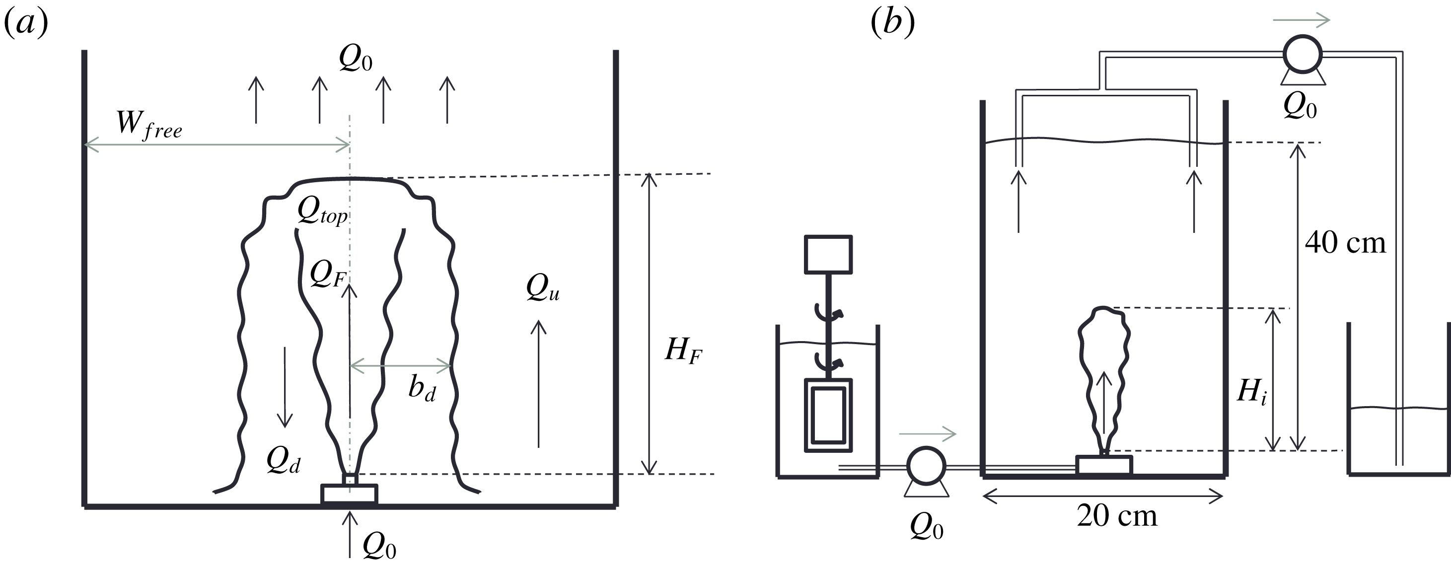
(Turner Reference Turner1966). A cartoon of a collapsed fountain is shown in figure 1(a), illustrating the up-flow in the fountain,
 $Q_{F}$
, the down-flow around the fountain,
 $Q_{d}$
, the resulting up-flow in the ambient,
 $Q_{u}$
, and the up-flow in the background above the top of the fountain,
 $Q_{0}$
. In an unconfined environment, the top of the fountain oscillates around the height
 $H_{F}$
. In a laterally confined environment, however, an upward flow develops in the ambient fluid, fed by the liquid spreading out from the fountain on the floor. Baines et al. (Reference Baines, Turner and Campbell1990) have investigated this fountain filling-box phenomenon for classical single-phase fountains in a homogeneous environment and Bloomfield & Kerr (Reference Bloomfield and Kerr1999) extended the work to account for a density-stratified environment. They found that when the volume flux supplied through the fountain was removed at high level above the fountain, the ambient layer of denser fluid always grows past the height of the fountain. The increasing density of the ambient fluid leads to a gradual decrease in the negative buoyancy flux of the fountain and hence an increase in fountain height.
(a) Cartoon of the collapsed fountain showing the fountain height,
 $H_{F}$
, and the volume fluxes in the fountain core,
 $Q_{F}$
, the down-flow,
 $Q_{d}$
, the up-flow outside the fountain,
 $Q_{u}$
and the volume flux above the top of the fountain,
 $Q_{0}$
. (b) Two-dimensional schematic of the experimental set-up: particles and fresh water are mixed together and pumped through a nozzle at the bottom of the tank (centre). A second pump extracts the liquid at the top of the tank to maintain a fixed reservoir level. The initial fluid leaving the nozzle reaches a maximum height
 $H_{i}$
(b) prior to the development of the collapsing fluid around the central jet, which leads to the lower quasi-steady fountain height
 $H_{F}$
(a). Once the filling-box flow develops in the ambient fluid some particles may be suspended, leading to an adjustment to a steady-state fountain height
 $H_{\infty }$
(§ 3.3).

In this paper we explore the filling-box dynamics of particle-laden fountains that results when a jet of particle-laden fluid enters an enclosed space filled with the same fluid. We first introduce the experimental method in § 2 and then present our experimental data and theoretical models, arranged into four regimes which depend on the terminal fall speed of the particles relative to the three characteristic velocities in the system.
2 Experimental method
We generated particle-laden fountains by supplying a mixture of fresh water and silicon-carbide particles to an upwards directed nozzle submerged in a tank of fresh water. The particles provide a buoyancy force which opposes the direction of the momentum flux at the source, thus producing a fountain. In this paper we present two groups of experiments. The first is a set of nine experiments for which all source conditions are fixed and only the particle size is varied between
 $12.8$
and
 $212~\unicode[STIX]{x03BC}\text{m}$
. The exact particle sizes and source conditions are listed in the upper part of table 1 (experiments a–i). The second is a set of 25 experiments with particle diameters between 12.8 and
 $30~\unicode[STIX]{x03BC}\text{m}$
. In this second set we also vary the nozzle diameter, source fluxes and particle concentration. These fountains have source Reynolds numbers between 1000 and 4000 and the initial Froude numbers range from 6 to 42. Three round stainless steel nozzles of internal diameter of approximately 2.9 mm, 5.2 mm and 8.5 mm were used as the sources. By repeating all experiments once, we estimate that the error in fountain height measurements in our experiments is somewhere close to 15 %. This error is comparable to the fountain height fluctuations of single-phase fountains around their mean height (Hunt & Burridge Reference Hunt and Burridge2015).
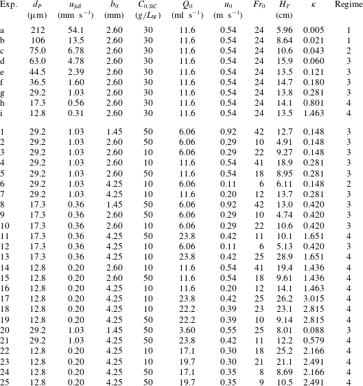
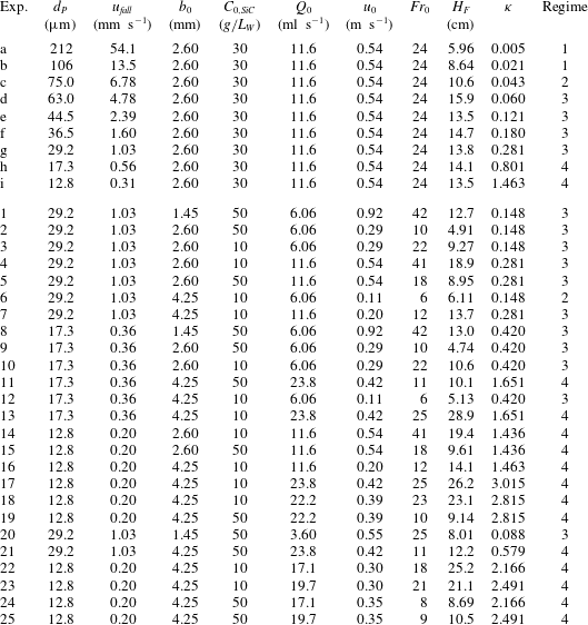
Table with source conditions for two sets of experiments on turbulent particle-laden fountains. In experiments a–i (above) all parameters except the particle size and thus
 $u_{fall}$
are kept constant. In experiments 1–25 (below) we vary the source momentum and buoyancy fluxes. The table lists the number of the experiment (Exp.), the particle diameter (
 $d_{P}$
), Stokes’ velocity of the particles (
 $u_{fall}$
), the nozzle radius (
 $b_{0}$
), the initial particle concentration (
 $C_{0}$
), the volume flux at the source (
 $Q_{0}$
), the nozzle exit velocity (
 $u_{0}$
), the source Froude number (
 $Fr_{0}$
), the fountain height (
 $H_{F}$
) and the ratio of background velocity to terminal particle settling velocity (
 $\unicode[STIX]{x1D705}$
).
The mixture of water and particles (Carborex F070 to F500 by Washington Mills) was pumped (Watson Marlow peristaltic pump) through a submerged nozzle at the bottom of a Perspex tank of dimensions
 $40~\text{cm}\times 20~\text{cm}\times 20~\text{cm}$
as shown in figure 1(b). An electroluminescent light sheet, connected to the back of the tank, provided uniform illumination for a JAI SP-5000 monochrome high-speed camera with a 1 : 28 HAMA lens. High-speed videos, eight minutes in length, with a frame rate of 10 Hz were recorded for all experiments. We use time-series images through the fountain centreline to extract the fountain height automatically.
3 Experimental observations: identification of four regimes
In our first set of experiments (table 1, a–i) all source conditions are fixed and we only vary the particle size and thus the terminal fall speed of the particles,
 $u_{fall}$
, as given by Stokes’ law for the small particles used herein,
 $$\begin{eqnarray}u_{fall}=\frac{2}{9}g\frac{\unicode[STIX]{x1D70C}_{P}-\unicode[STIX]{x1D70C}_{W}}{\unicode[STIX]{x1D707}_{W}}\frac{d_{P}^{2}}{4},\end{eqnarray}$$
where
 $\unicode[STIX]{x1D70C}_{P}=3.21~\text{g}~\text{cm}^{-3}$
is the density of the silicon-carbide particles,
 $\unicode[STIX]{x1D70C}_{W}\approx 1~\text{g}~\text{cm}^{-3}$
is the density of the ambient water and
 $\unicode[STIX]{x1D707}_{W}\approx 1~\text{mPa}~\text{s}$
is the dynamic viscosity of water at room temperature. The Reynolds number of the particles based on their fall speed and radius is always much smaller than 10 (much smaller than 0.1 for experiments 1–25).
We find that the fate of the particles depends on the relative magnitude of
 $u_{fall}$
compared to three distinct up-flow velocities. These are (i) the up-flow velocity within the fountain core as quantified by the characteristic fountain velocity,
 $u_{F}=B_{0}^{1/2}M_{0}^{-1/4}$
, (ii) the maximum upward filling-box speed in the ambient fluid which occurs at the base of the fountain,
 $u_{u}(0)$
, and (iii) the up-flow velocity above the top of the fountain,
 $u_{BG}$
, which results from the source flux,
 $u_{BG}=Q_{0}/A$
, where
 $Q_{0}=\unicode[STIX]{x03C0}q_{0}=\unicode[STIX]{x03C0}b_{0}^{2}u_{0}$
is the source volume flux and
 $A$
is the cross-sectional area of the tank. Based on the ratios
 $u_{F}/u_{fall},u_{u}(0)/u_{fall}$
and
 $u_{BG}/u_{fall}$
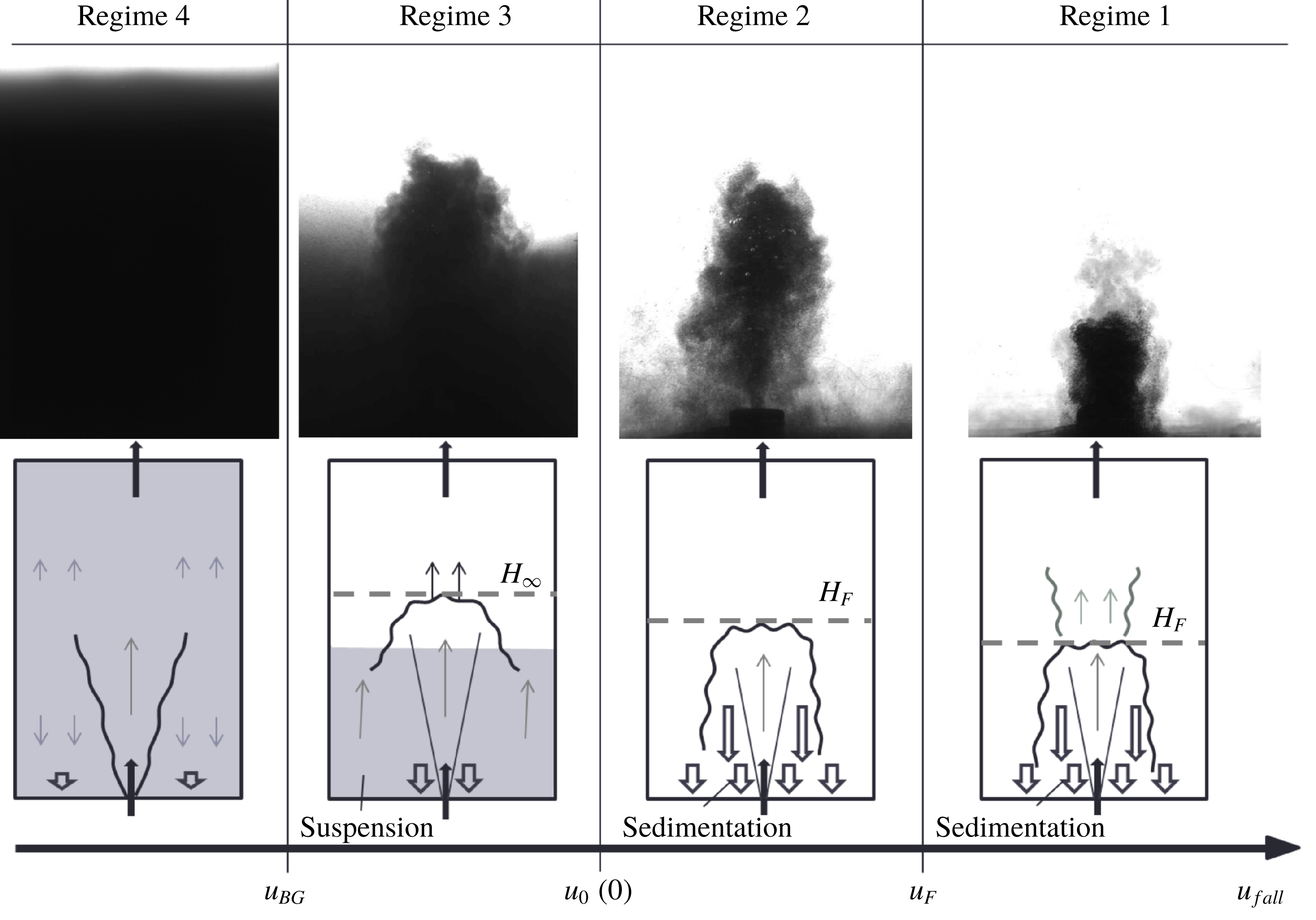
, we identify four regimes which are illustrated in figure 2 and described in the following sections.
Regime diagram with images from four experiments (Regime 1, exp. a; Regime 2, exp. c; Regime 3, exp. g; Regime 4, exp. i) and accompanying schematics describing the quasi-steady-state observations for the four distinct regimes. The regimes depend on the relative magnitude of
 $u_{fall}$
compared to the characteristic fountain velocity,
 $u_{F}$
, the maximum up-flow speed outside the fountain,
 $u_{u}(0)$
, and the background velocity,
 $u_{BG}$
. In the experimental image of the separated flow regime (Regime 1), some dye has been added to the source liquid to show that the particles separate from the flow when the fountain liquid still has some upward momentum.

3.1 Regime 1:
 $u_{fall}>u_{F}$
, the separated two-phase fountain

If
 $u_{fall}$
exceeds the characteristic fountain velocity,
 $u_{F}$
, the particles separate from the fountain liquid and fall out of the fountain before the liquid runs out of momentum. Mingotti & Woods (Reference Mingotti and Woods2016) found that the maximum height reached by the particles in a particle-laden fountain,
 $H_{F}$
, decreases compared to the height of an equivalent single-phase fountain,
 $H_{SPF}$
, if
 $\unicode[STIX]{x1D6EC}=u_{fall}/u_{F}>0.25$
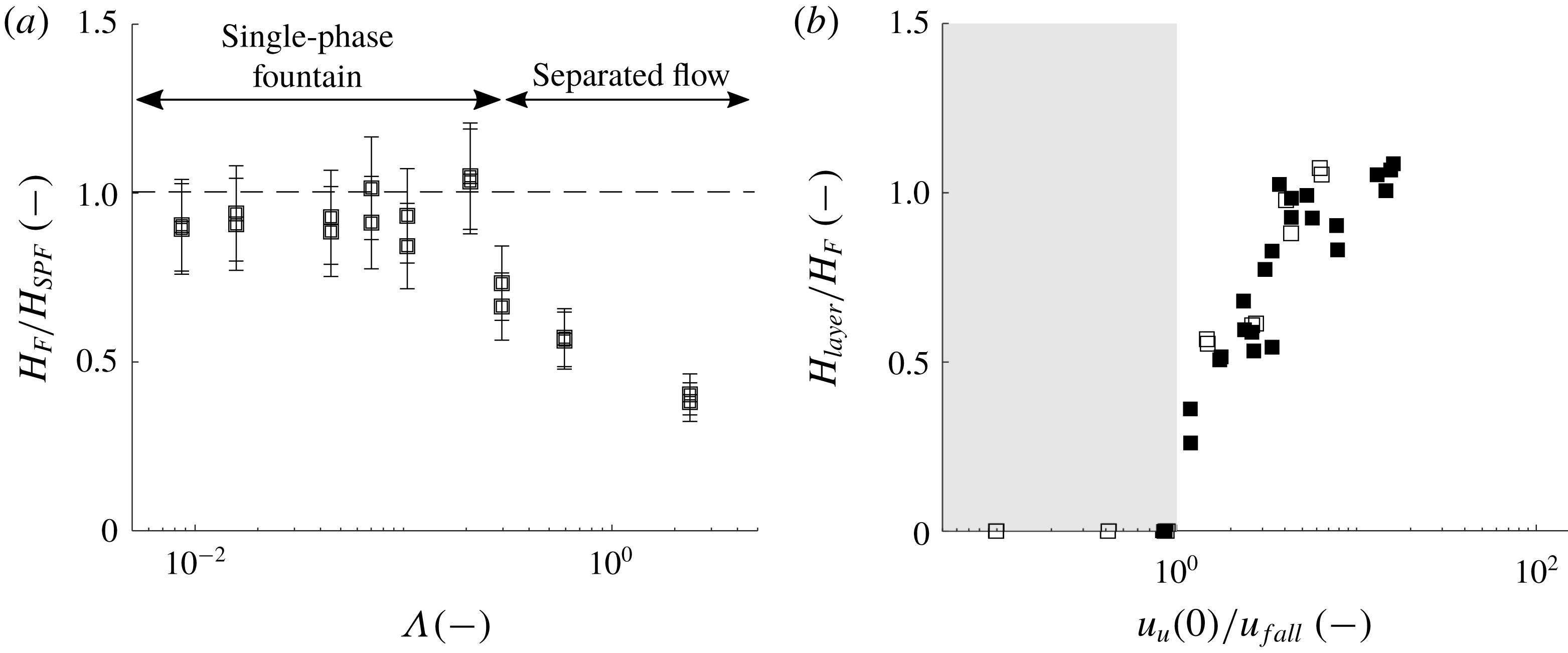
. Figure 3(a) illustrates the variation of
 $H_{F}/H_{SPF}$
as a function of
 $\unicode[STIX]{x1D6EC}$
for experiments a–i, and our observations are consistent with the results of Mingotti & Woods (Reference Mingotti and Woods2016).
(a) Ratio of the quasi-steady fountain height,
 $H_{F}$
, as a fraction of the height of an equivalent single-phase fountain,
 $H_{SPF}$
(1.1), for experiments a–i as listed in table 1. This ratio is shown as a function of
 $\unicode[STIX]{x1D6EC}=u_{fall}/u_{F}$
. The height of the particle-laden fountain is comparable to a single-phase fountain if
 $u_{fall}<0.25u_{F}$
, but decreases as
 $\unicode[STIX]{x1D6EC}$
increases to larger values and the effects of separated flow become increasingly important (Mingotti & Woods Reference Mingotti and Woods2016). (b) Variation of the ratio of particle layer height in the ambient to the quasi-steady fountain height,
 $H_{layer}/H_{F}$
, as a function of
 $u_{u}(0)/u_{fall}$
for all experiments for which
 $u_{fall}>u_{BG}$
. For
 $u_{u}(0)/u_{fall}<1$
(region shaded in grey), no layer is observed. Experiments a–i are plotted as empty squares; the remainder of the experiments are shown as solid squares.

3.2 Regime 2:
$u_{F}>u_{fall}>u_{u}(0)$
, no filling-box

For
 $\unicode[STIX]{x1D6EC}=u_{fall}/u_{F}<0.25$
, particle-laden fountains behave like the analogous single-phase fountain of the same buoyancy and momentum flux and the particles are carried to the top of the fountain. However, if
 $u_{fall}$
is larger than the maximum filling-box speed in the ambient,
 $u_{fall}>u_{u}(0)$
, the particles quickly settle to the floor. No particles are suspended in the environment and the fountain reaches a quasi-steady height,
 $H_{F}$
. The maximum filling-box speed,
 $u_{u}(0)$
, can be estimated by considering the total volume flux in the fluid which collapses back down to the base of the tank around the central up-flowing fountain. Burridge & Hunt (Reference Burridge and Hunt2016) have measured the total volume flux of the collapsing fluid at the level of the source,
 $Q_{d}(0)$
, and based on their data for
 $Fr_{0}>2$
they proposed the empirical law
 $$\begin{eqnarray}Q_{d}(0)=Q_{0}(1+0.71Fr_{0}).\end{eqnarray}$$
The upward filling-box flow,
 $Q_{u}$
, and the upward filling-box velocity,
 $u_{u}$
, are then given by the mass balance
 $$\begin{eqnarray}Q_{u}(z)=A_{free}u_{u}(z)=Q_{d}(z)-Q_{F}(z)+Q_{0},\end{eqnarray}$$
where
 $A_{free}=A-A_{F}$
is the available area for the up-flow.
 $A$
is the area of the enclosed space and
 $A_{F}$
the area of the fountain. Mizushina et al. (Reference Mizushina, Ogino, Takeuchi and Ikawa1982) have shown experimentally that the radius of a collapsing fountain is constant at approximately
 $b_{d}=0.37H_{F}$
so that
 $A_{F}=\unicode[STIX]{x03C0}b_{d}^{2}$
. In figure 3(b) the region where
 $u_{fall}>u_{u}(0)$
is shaded in grey. This panel contains a plot of the ratio of measured particle layer height as a fraction of the fountain height,
 $H_{layer}/H_{F}$
, as a function of the velocity ratio
 $u_{u}(0)/u_{fall}$
. The graph illustrates that for
 $u_{fall}>u_{u}(0)$
no layer is observed. For
 $u_{fall}<u_{u}(0)$
, however, a particle layer does form and becomes progressively deeper as
 $u_{u}(0)/u_{fall}$
increases. This is discussed in the following sections.
3.3 Regime 3:
$u_{u}(0)>u_{fall}>u_{BG}$
, trapped filling-box

If the particle fall speed is smaller than the maximum up-flow velocity outside the fountain but exceeds the background velocity above the top of the fountain,
 $u_{BG}<u_{fall}<u_{u}(0)$
, a particle layer develops around the fountain and extends from the floor to some height smaller than the fountain height. The presence of the particle-rich layer in this regime reduces the effective negative buoyancy flux in the fountain. Consequently, the fountain height increases from the quasi-steady height prior to the development of the particle-laden layer,
 $H_{F}$
, to a new steady-state fountain height,
 $H_{\infty }$
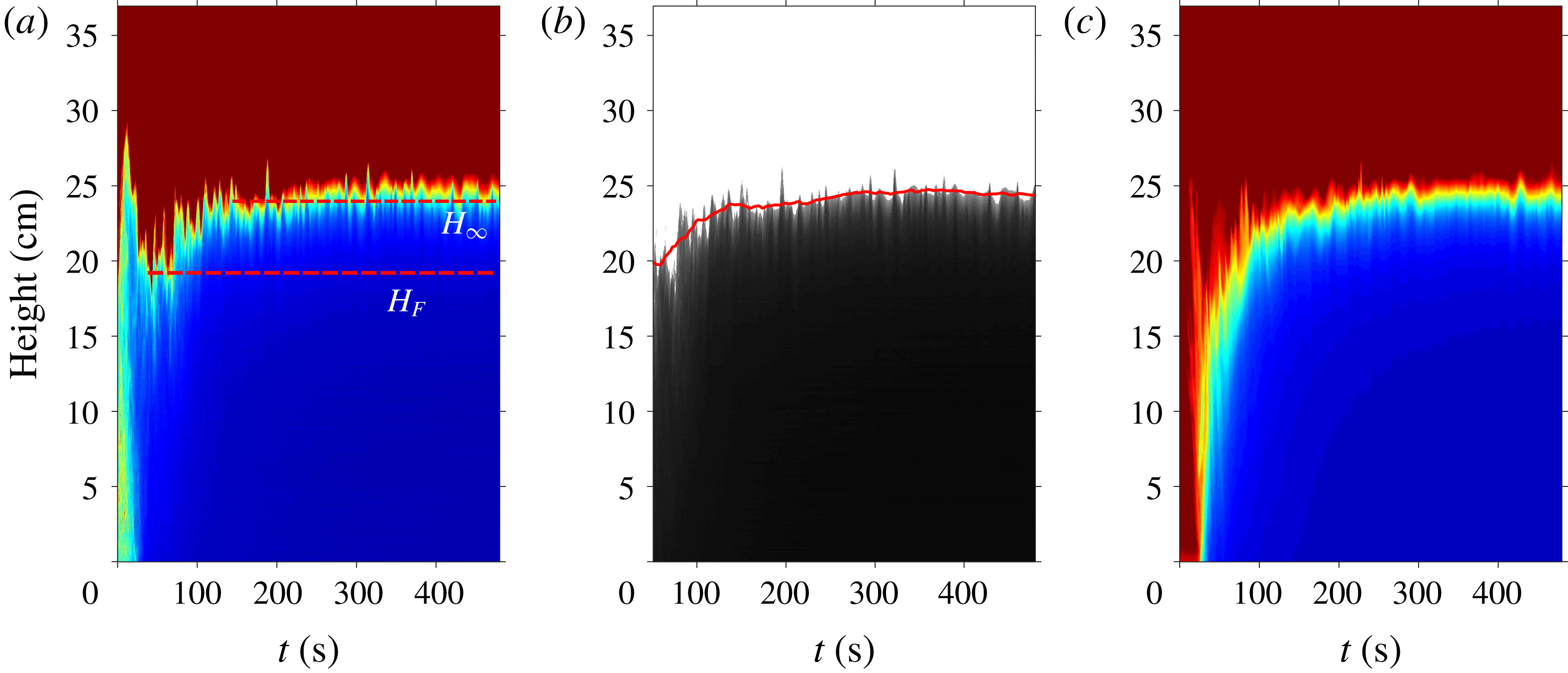
. Figure 4(a) contains an experimental time-series image describing the evolution of a single vertical line of pixels, through the centre of a fountain, as a function of time. The initial starting fountain flow reaches a height of approximately 29 cm, but after approximately 10 s the fountain collapses and adjusts to a quasi-steady height of approximately
 $H_{F}=20$
cm. The filling-box process then becomes established over the next 200 s (c), and the fountain height gradually rises to
 $H_{\infty }\approx 24$
cm. Both the initial quasi-steady fountain height,
 $H_{F}$
, and the increased fountain height,
 $H_{\infty }$
, are marked in (a). Both
 $H_{F}$
and
 $H_{\infty }$
were determined automatically by detecting the top of the fountain from the time-series image through the fountain centre (a) after the initial fountain collapse. The random oscillations of the fountain top were averaged by considering a fountain height averaged over a 10 s period as shown by the red line in figure 4(b). The initial averaged height corresponds to
 $H_{F}$
, and the final averaged height is taken to be
 $H_{\infty }$
. The averaging period over which the running mean fountain height was computed (red line (b)) was chosen to be large compared to the time scale over which the fountain top oscillates, but small compared to the time scale over which the filing-box flow in the background becomes established. In our experiments the time scale of fountain height fluctuation is of the order of seconds, and the time scale over which a particle layer develops in the ambient is closer to 100 seconds. We chose an averaging period of 10 seconds, but we find that averaging periods in the range 5–20 s yield similar values for
 $H_{F}$
and
 $H_{\infty }$
.
(a) Time-series image in false colour of a vertical line through the centre of the fountain obtained for experiment 4 in table 1. The overshoot fountain height,
 $H_{i}\approx 29$
cm, after 10 s is followed by the quasi-steady fountain height,
 $H_{F}$
, after approximately 30 s. As the filling-box flow develops (c) the fountain height increases to the steady-state fountain height,
 $H_{\infty }$
. (b) Illustration of the automated extraction of
 $H_{F}$
and
 $H_{\infty }$
by computing the average fountain height over a period of 10 seconds, as shown by the red line. (c) Time-series image of horizontally averaged light intensity outside the fountain illustrating the development of the particle layer in the background around the fountain.

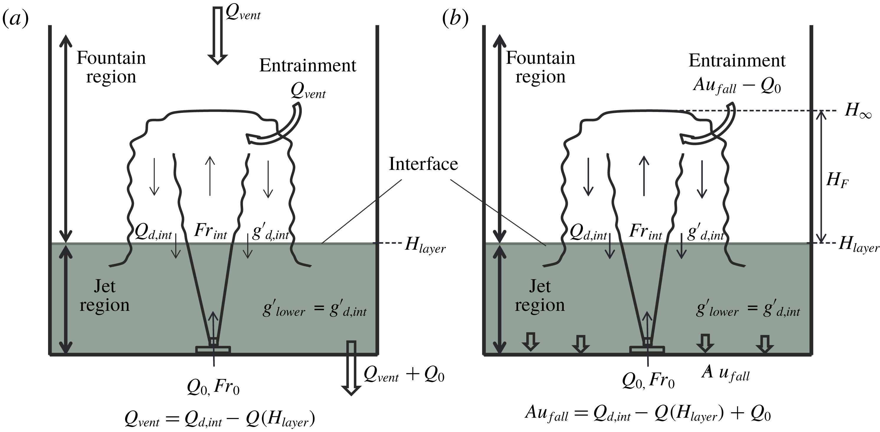
(a) Cartoon illustrating the experimental set-up and key results of Baines et al. (Reference Baines, Corriveau and Reedman1993) on single-phase fountains in a confined ventilated space. The height of the interface at
 $z=H_{layer}$
is fixed. In the lower layer, the flow issuing through the nozzle resembles a negatively buoyant jet. Above the interface, the flow transitions into a turbulent fountain. The entire ventilation flux,
 $Q_{vent}$
, is entrained into the fountain above the interface. The buoyancy of the collapsing down-flow matches the buoyancy in the lower layer. (b) In Regime 3 a particle-laden layer forms which extends from the bottom of the tank to a height
 $z=H_{layer}$
. Motivated by Baines et al. (Reference Baines, Corriveau and Reedman1993) we model the flow in the lower layer as a negatively buoyant jet which transitions into a fountain as it passes upwards through the interface. The buoyancy of the downward return flux equals the buoyancy in the lower layer. Some fraction of the collapsing particle flux is re-entrained into the fountain; the remainder settles on the floor.

In order to calculate the height of rise of the fountain, we require a model that considers the ascent of a fountain which initially rises through the particle-laden layer of ambient fluid, but which then adjusts owing to the rapid increase in the negative buoyancy flux as it rises into the particle-free layer above. In our investigation of this process we are guided by previous studies on single-phase salt water fountains in a two-layer stratified environment (Baines et al.
Reference Baines, Corriveau and Reedman1993; Ansong et al.
Reference Ansong, Kyba and Sutherland2008). To help guide our understanding, in figure 5(a) we show the key results presented by Baines et al. (Reference Baines, Corriveau and Reedman1993). They produced single-phase fountains in a closed, ventilated space in which a constant flux of ambient fluid was removed from the tank at the level of the source. This led to the development of a counter-flow in the tank, opposing the direction of the initial momentum of the fountain. A stable interface develops at the height where the total entrainment into the fountain above the interface matches the volume flux of fluid removed from the tank (minus the source flux
 $Q_{0}$
) at the elevation of the source. At large times, the buoyancy flux entering the tank through the nozzle is balanced by the total buoyancy flux of the liquid flux removed from the tank,
 $$\begin{eqnarray}g_{0}^{\prime }Q_{0}=g_{lower}^{\prime }(Q_{vent}+Q_{0}),\end{eqnarray}$$
where
 $g_{lower}^{\prime }$
is the buoyancy in the lower layer and
 $Q_{vent}$
is the volume flux of the ventilation flow. The authors further establish that at the height of the interface between the two layers, the buoyancy of the downward collapsing flow which is shed from the top of the fountain,
 $g_{d,int}^{\prime }$
, matches
 $g_{lower}^{\prime }$
. Hence, below the interface, they do not observe a strong return flow around the fountain core. We have repeated their experiments and show the results in figure 6. Panel (a) shows an image of the single-phase salt water fountain after the initial collapse. Panel (b) shows the fully developed two-layer stratification owing to the background flux in the tank. The colour of the source liquid is changed in (c) and (d) to monitor the flow path of the fountain fluid. We observe that upon entering the lower layer, the downward collapsing flow spreads out horizontally throughout the depth of the lower layer.
Images of single-phase fountains in a ventilated enclosure. (a) A single-phase salt water fountain (
 $H_{F}\approx 8$
cm) is produced in a fresh water tank. (b) The background ventilation rate,
 $Q_{vent}$
, is adjusted (cf. Baines et al.
Reference Baines, Corriveau and Reedman1993) such that a stable two-layer stratification develops in the ambient. (c) In steady state, the colour of the source liquid is changed to visualise the flow path of the fountain fluid. (c,d) The source liquid rises to the top of the fountain, collapses and spreads out at all heights around the fountain. A strong return flow, as characteristic for a fountain, is not observed in the lower layer.

In the present experiments, by analogy, we envisage that the fountain fluid falling into the particle layer has the same buoyancy as this layer and so it spreads out horizontally into this layer, in a similar fashion to the saline fountain (figure 6). Owing to the absence of a return flow in the lower layer, we model the flow produced by the jet issuing from the source as a particle-laden jet with negative buoyancy. However, once this jet penetrates the interface with the particle-free layer, we assume that the flow transitions to a turbulent fountain. The source conditions of this fountain correspond to the previously calculated jet properties just above the interface. The equations for the conservation of volume, buoyancy and momentum fluxes of a negatively buoyant jet in a uniform environment and their respective changes in the direction of the vertical coordinate
 $z$
are
 $$\begin{eqnarray}Q(z)=\unicode[STIX]{x03C0}b(z)^{2}u(z),\quad \frac{\text{d}Q(z)}{\text{d}z}=\unicode[STIX]{x1D6FC}2\unicode[STIX]{x03C0}b(z)u(z),\end{eqnarray}$$
 $$\begin{eqnarray}B(z)=\unicode[STIX]{x03C0}b(z)^{2}u(z)g^{\prime }(z),\quad \frac{\text{d}B(z)}{\text{d}z}=0,\end{eqnarray}$$
 $$\begin{eqnarray}M(z)=\unicode[STIX]{x03C0}b(z)^{2}u(z)^{2},\quad \frac{\text{d}M(z)}{\text{d}z}=-\unicode[STIX]{x03C0}b(z)^{2}g^{\prime }(z),\end{eqnarray}$$
as described by Morton et al. (Reference Morton, Taylor and Turner1956), where we adopt the horizontally averaged top-hat model for the jet properties as well as the entrainment hypothesis which states that the entrainment of ambient liquid into the jet is proportional to the local jet velocity at any height. The constant of proportionality is taken to be
 $\unicode[STIX]{x1D6FC}\approx 0.076$
(Bloomfield & Kerr Reference Bloomfield and Kerr2000).
For the present experiments on particle-laden fountains the analogue to the volume flux removed from the tank at the height of the source,
 $Q_{vent}+Q_{0}$
, is the settling of particles at the bottom of the tank. The buoyancy of the lower layer may thus be determined as
 $$\begin{eqnarray}g_{lower}^{\prime }=\frac{g_{0}^{\prime }Q_{0}}{Au_{fall}},\end{eqnarray}$$
as illustrated by the cartoons in figure 5(a,b). The effective buoyancy of the negatively buoyant jet in the lower layer becomes
 $g_{0,eff}^{\prime }=g_{0}^{\prime }-g_{lower}^{\prime }$
. The height of the top of the fountain which forms as the negatively buoyant jet rises through the interface into the particle-free fluid is given as the sum of the interface height,
 $H_{layer}$
, and the height of a turbulent fountain in the upper layer,
 $H_{F,upper}$
, with the source conditions matching the properties of the jet just above the interface,
 $$\begin{eqnarray}H_{\infty ,theo}=H_{layer}+H_{F,upper}.\end{eqnarray}$$
Hunt & Burridge (Reference Hunt and Burridge2015) have published a detailed set of experiments with empirical relationships between the quasi-steady rise height of turbulent fountains as a function of the source radius of the jet and the Froude number for very weak fountains (
 $0.3<Fr_{0}<1$
), weak fountains (
 $1<Fr_{0}<2$
), intermediate fountains (
 $2<Fr_{0}<4$
) and forced fountains (
 $Fr_{0}>4$
, see (1.1)). We adopt these relationships to compute a theoretical estimate of the total fountain height in the upper layer, based on the jet radius just above the interface,
 $b_{int}$
, and the corresponding Froude number, defined in terms of the density difference of the fountain and the upper layer fluid,
 $g_{int}^{\prime }$
, the jet velocity just above the interface,
 $u_{int}$
, and the jet radius so that
 $Fr_{int}=u_{int}/\sqrt{g_{int}^{\prime }b_{int}}$
. In turn the values of
 $b_{int}$
,
 $u_{int}$
and
 $g_{int}^{\prime }$
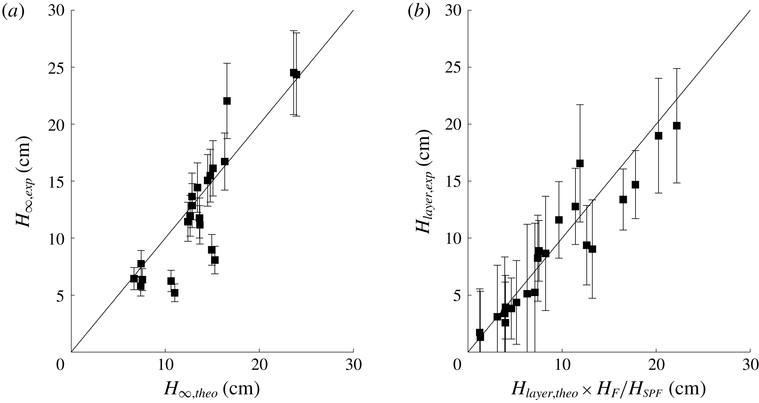
at the interface are calculated by numerical solution of the jet equations ((3.5)–(3.7)) with the actual source conditions at the inflow nozzle, using the result in (3.4) to determine the effective buoyancy of the incoming jet. The results are shown in figure 7(a) where we plot the experimentally determined total fountain height,
 $H_{\infty ,exp}$
, on the
 $y$
-axis as a function of the corresponding theoretical estimate for the fountain height,
 $H_{\infty ,theo}$
on the
 $x$
-axis. Most data points (black squares) are in reasonable agreement with the solid black line which has a gradient of one.
(a) Comparison of the experimental measurements of total fountain height in the two-layer stratification,
 $H_{\infty ,exp}$
, on the
 $y$
-axis, and the theoretical estimate of this height,
 $H_{\infty ,theo}$
on the
 $x$
-axis. (b) Plot of the measured height of the interface,
 $H_{layer,exp}$
, on the
 $y$
-axis as a function of the theoretical estimate of the layer height,
 $H_{layer,theo}$
, corrected by the ratio
 $H_{F}/H_{SPF}$
, on the
 $x$
-axis.

A theoretical estimate of the height of the interface between the lower and the upper layer in steady state,
 $H_{layer}$
, was obtained by matching the mass flux of the particles in the collapsing down-flow of the fountain above the interface with the settling flux of particles at the floor of the tank. Since the concentration of particles in the collapsing down-flow matches that in the lower layer, this balance reduces to the simple form
 $$\begin{eqnarray}Q_{d,int}-Q(H_{layer})+Q_{0}=Au_{fall}.\end{eqnarray}$$
The cartoons in figure 5(a,b) illustrate that
 $Q_{d,int}$
is the total volume flux of the collapsed fountain at the height of the interface. Burridge & Hunt (Reference Burridge and Hunt2016) provide a detailed set of empirical laws relating the total volume flux of a turbulent single-phase fountain as it collapses and falls past the original height of the input nozzle to the source Froude number. We use this relation to compute the total flux of collapsing fountain fluid,
 $Q_{d,int}$
, by first solving the jet equations for each interface height. We then employ the empirical relationships to determine the value of
 $Q_{d,int}$
for each iteration of
 $H_{layer}$
. We take the interface height at which
 $Q_{d,int}-Q(H_{layer})+Q_{0}$
first decreases below
 $Au_{fall}$
as our theoretical estimate of the layer height,
 $H_{layer,theo}$
. In figure 7(b) the measured fountain height,
 $H_{layer,exp}$
, is plotted as a function of the theoretically estimated layer height, corrected by the ratio of measured fountain height and single-phase fountain height. The experimental data are compared with the theoretical prediction (black solid line of gradient one).
3.4 Regime 4:
$u_{fall}>u_{BG}$
, unbounded filling-box

When the terminal particle fall speed falls below the background velocity,
 $u_{fall}<u_{BG}$
, particles are lifted above the top of the fountain and a particle front gradually fills the entire tank. The relative magnitude of the particle fall speed to the background velocity may be expressed in terms of the dimensionless parameter
 $\unicode[STIX]{x1D705}$
,
 $$\begin{eqnarray}\unicode[STIX]{x1D705}=\frac{Q_{0}}{Au_{fall}}.\end{eqnarray}$$
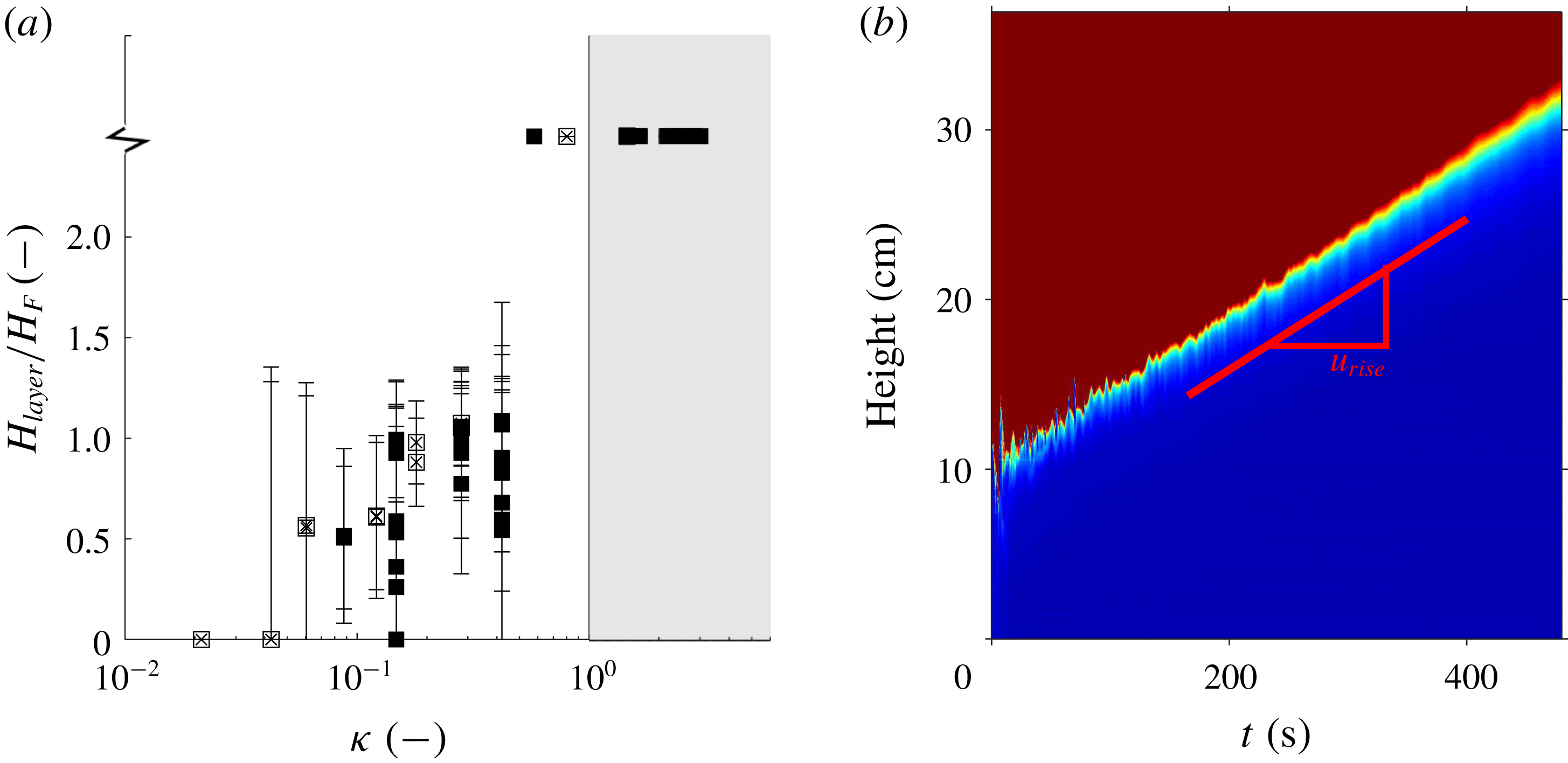
Figure 8(a) contains a plot of the ratio of measured particle layer height to quasi-steady fountain height,
 $H_{layer}/H_{F}$
, as a function of
 $\unicode[STIX]{x1D705}$
. The region
 $\unicode[STIX]{x1D705}>1$
is shaded in grey. In this regime the front rises and gradually fills the entire tank. Some experiments with
 $\unicode[STIX]{x1D705}$
close to but smaller than one also led to the development of a particle-rich layer above the top of the fountain as shown in figure 8(a). This is the result of the finite size distribution of the particles used in the experiments, such that even if the mean particle fall speed exceeds the background speed,
 $u_{BG}$
, there is a non-negligible fraction of the particles for which
 $u_{fall}<u_{BG}$
and hence which are carried upwards to the high level vent in the tank. Similarly, the scatter in the region
 $\unicode[STIX]{x1D705}<1$
is associated with the range of particle sizes, resulting in a diffuse front. The error bars illustrate the difference in layer height measurement between the uppermost front (where we first record a reduction in light intensity) and the layer height at which no light passes through the particle layer.
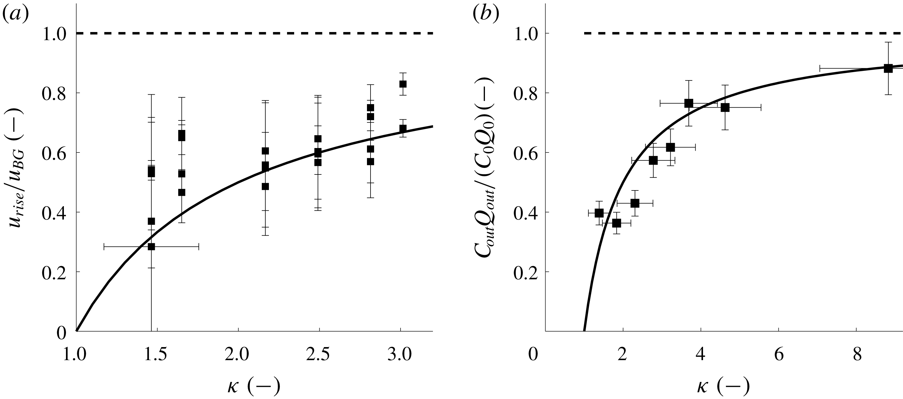
An example of the ascending front of the particle layer is displayed in the experimental time-series image shown in figure 8(b). By extracting the slope of the propagating fronts in such time-series images we may estimate the filling-box speed. Figure 9(a) illustrates the ratio of measured front velocity and the background velocity,
 $u_{rise}/u_{BG}$
, as a function of
 $\unicode[STIX]{x1D705}$
. The solid black line corresponds to the background velocity minus
 $u_{fall}$
,
 $$\begin{eqnarray}u_{rise}=u_{BG}-u_{fall}.\end{eqnarray}$$
We observe that the measured rise speeds are described reasonably well by (3.12). Again, the scatter is associated with the range of particle sizes, resulting in a diffuse front.
To check for consistency we ran a series of equivalent single-phase fountain experiments for the source conditions of experiments 1–25 and found that the measured front velocities corresponded to the background velocity,
 $u_{BG}$
, within an error of less than 8 %. In figure 9(a), these data points would lie on the dashed horizontal line.
(a) Variation of the ratio of the depth of the particle layer as a fraction of the quasi-steady fountain height,
 $H_{F}$
, as measured for all experiments shown in table 1. The ratio is shown as a function of
 $\unicode[STIX]{x1D705}$
, the ratio of the background flow speed above the top of the fountain and the terminal particle fall speed. Open symbols correspond to experiments a–i and solid symbols represent experiments 1–25. For
 $\unicode[STIX]{x1D705}>1$
the interface height rises indefinitely. (b) Time-series image in false colour through the centre of the fountain obtained for experiment 13 in table 1. The particle-laden layer (blue) surpasses the quasi-steady fountain height,
 $H_{F}$
, after approximately 30 s, after which the front gradually fills the entire tank.

(a) Plot of the ratio of the measured particle-laden front velocity to the background velocity,
 $u_{rise}/u_{BG}$
, as a function of
 $\unicode[STIX]{x1D705}$
. The solid line corresponds to the prediction
 $u_{rise}=u_{BG}-u_{fall}$
. (b) Measurement of the ratio of the vented particle flux,
 $C_{out}Q_{out}$
, and the total volume flux supplied to the tank,
 $C_{0}Q_{0}$
, plotted as a function of
 $\unicode[STIX]{x1D705}$
for
 $\unicode[STIX]{x1D705}>1$
. The solid black line corresponds to the theory.

In this regime, the influx of particles,
 $Q_{P}$
, is balanced by both the flux of particles settling at the bottom of the tank (first term on the right-hand side) and the flux of particles vented through the outflow at the top of the tank (second term on the right-hand side),
 $$\begin{eqnarray}Q_{P}=C_{0}Q_{0}=C_{E}Au_{fall}+C_{E}(Q_{0}-Au_{fall}),\end{eqnarray}$$
where we assume the particle concentration in the ambient fluid,
 $C_{E}$
, is uniform. From (3.13) we infer that the particle concentration in the ambient matches the particle concentration at the source,
 $$\begin{eqnarray}C_{E}=C_{0}.\end{eqnarray}$$
As a result of this equality, the flow issuing from the nozzle now resembles a neutrally buoyant jet. Unfortunately, in this regime the particles in the background flow block the view of the fountain so we have not been able to visualise the flow issuing from the source. However, we have tested the prediction of (3.14) by running eight experiments in which we collect the outflow from the top of the tank. The weight of the total mixture of water and particles was measured as well as the weight of only the particles after a drying process, in order to determine the flux of particles issuing from the tank,
 $C_{out}Q_{out}$
. The ratio of the vented particle flux to the total particle flux may thus be written as
 $$\begin{eqnarray}\frac{C_{0}\,(Q_{0}-Au_{fall})}{C_{0}\,(Q_{0}-Au_{fall})+C_{0}Au_{fall}}=1-\frac{1}{\unicode[STIX]{x1D705}}.\end{eqnarray}$$
The prediction of this model is shown as a solid black line in figure 9(b) and appears to be in reasonable agreement with our experimental measurements. This result is in agreement with our previous finding that the particle-laden front rises with the velocity
 $u_{rise}=u_{BG}-u_{fall}$
.
4 Summary
We have studied the transport of particles supplied to a confined environment as a particle-laden fountain. We have identified four distinct regimes by comparing the terminal particle fall speed,
 $u_{fall}$
, against the up-flow velocities in the fountain core, outside the fountain, and in the background above the top of the fountain. In Regime 1, the particles separate from the fountain liquid. In Regime 2, all particles are carried to the top of the fountain, but very quickly settle from the collapsing down-flow and do not form a particle layer in the ambient. In Regime 3, we observe a trapped particle-rich layer in the ambient fluid. This reduces the density difference between fountain and environment and encourages larger fountain heights. In Regime 4, the background flow is strong enough to lift particles above the top of the fountain and the entire tank eventually fills with particles. Novel experimental data are complemented by simple models which predict (i) whether or not a particle-rich layer develops in the ambient, (ii) the height of the contaminated layer, (iii) the increase in fountain height owing to the presence of the particle-rich layer, (iv) the velocity of the rising particle layer front for
 $\unicode[STIX]{x1D705}>1$
and (v) the concentration of particles in the ambient for
 $\unicode[STIX]{x1D705}>1$
. This work provides a framework for interpreting the fate of particles carried by liquid jets in a confined space.
It would be of great interest to develop the models and experiments introduced herein to suspensions of multiple sizes, both in terms of the dynamics and also the potential for a novel separation system.
Acknowledgements
This work was funded through the BP Institute, a Benefactors’ Scholarship from St John’s College Cambridge and an EPSRC Industrial CASE Award.