Between the summer of 1937 and the spring of 1938 the US economy experienced the steepest slump in its history. Industrial production fell by more than 30 per cent, the stock market index dropped by nearly 40 per cent, and the unemployment rate increased from 15 to 19 per cent.Footnote ² The Bank for International Settlements (BIS), alarmed by the quick reversal after August 1937, noted that US industrial production ‘showed an almost vertical drop’ which was ‘greater than in the autumn of 1929’ (BIS 1938, p. 6). And with the US economy still being the largest economy of the world, the impact was immediately felt all over the world. According to the BIS the decline in some countries outside the US was ‘so marked that a parallel can be found only in the most acute depressions ever known’ (BIS 1938, p. 6). The world, many contemporaries feared, was on the brink of another economic disaster. Yet, while the dramatic fall of US industrial production sent shockwaves across the world, the global recession proved to be surprisingly mild. The decline of world GDP in 1938 amounted to only 0.4 per cent compared to 3.6 per cent in 1930. The US recession had its impact, but the fear of another depression proved overly pessimistic. Recovery was in full swing by the end of 1938.

Why were the global repercussions of the US slump in 1938 less severe than in 1930? The standard view is that all major countries had abandoned the gold standard and enjoyed more policy freedom. Accordingly, Germany and Japan were shielded by tight capital controls and therefore able to maintain their high level of defence spending, Britain could start a big rearmament programme and absorb the deflationary shock of the US economy thanks to its floating exchange rate regime, and a number of other countries, namely in Europe and Latin America, reacted to the US slump by introducing capital controls or letting their currencies depreciate (Eichengreen Reference Eichengreen1992, pp. 386–9).

This article challenges the standard view. While it is beyond doubt that Germany and a couple of Central and Eastern European countries were in fact able to protect themselves by maintaining or imposing tight capital controls, most countries were still constrained by their golden fetters. Britain and the sterling bloc as well as a number of small countries did not have much room for manoeuvre when the US recession affected the world economy. Most members of the sterling bloc – in particular Australia and India – defended and kept their sterling parities while in 1929–30 they had devalued their currencies. Neither was the British rearmament programme too big to violate the rules of the gold standard. Additionally, the fact that some Latin American countries let their currencies weaken is not an argument for a reformed international monetary system; they had pursued the same exchange-rate policy in 1929–30.

We obtain supporting results from a de facto classification of exchange-rate regimes during the interwar years, tests on the effectiveness of capital controls and a descriptive analysis of British fiscal policy in the 1930s. The classification suggests that most countries in the 1930s quickly returned to fixed exchange-rate regimes after halting gold convertibility. They had broken their golden fetters in order to devalue their currencies, not to abandon the gold standard altogether. Germany is an exception, not a typical case; most countries with capital controls loosened them over the course of the decade, in part because they did not have the means to enforce them (Gordon Reference Gordon1941). The global reserve position improved thanks to large-scale devaluations of all major currencies and their major trading partners between 1931 and 1936.

This article has implications for the conventional view of the international monetary system of the interwar years. The 1930s should be viewed as a key link between the gold standard and Bretton Woods rather than a temporary digression from fixed exchange rates. The 1944 agreement in New Hampshire codified what had already become common practice in the 1930s. From a longer-term viewpoint, floating currencies based on fiat money would have to await the collapse of the Bretton Woods system in the early 1970s. This was the key twentieth-century paradigm shift in the international monetary system.

The article has five parts. Section I discusses parallels and differences between 1929–30 and 1937–8 in the US and at the global level and summarises the standard view of why there was no global recession in 1938. Sections II and III present our classification scheme of exchange-rate regimes and capital controls, illustrated by some country examples. Section IV discusses the British case by comparing the freedom of fiscal policy under the classical gold standard and in the late 1930s. The concluding section highlights implications for the history of the international monetary system between the gold exchange standard and Bretton Woods.

I

In early 1937, the outlook for the world economy could not have been better. The BIS observed in its annual report that ‘for the first time since the beginning of the depression practically every important sphere of business has been brought into the upward movement’ (BIS 1937, p. 5). World industrial production and the physical volume of global trade had finally approached the level of 1929 (Lary Reference Lary1943, pp. 183 and 186). Also, the threat of deflation had become much weaker. In 1936, world prices for food and raw materials had increased for the first time since the beginning of the crisis, and world prices for manufactures were at least not falling anymore (Feinstein, Temin and Toniolo Reference Feinstein, Temin and Toniolo1997, p. 171). And finally, tensions within the international monetary system had become less serious since the devaluation of the French, Dutch and Swiss currencies and the conclusion of the Tripartite Agreement in September 1936.

Just as the sense of relief was growing, the US economy experienced a severe setback. From July 1937 to May 1938 industrial production declined by 31 per cent, the Dow Jones Industrial Average by 39 per cent.Footnote ³ And as the economic contraction immediately affected the labour market – the unemployment rate jumped from 15 to 19 per cent – the ruling Democrats were promptly punished in the mid-term elections of November 1938.Footnote ⁴ For the first time since 1928 they lost seats both in the House of Representatives and the Senate (Freidel Reference Freidel1990, p. 250). The unexpected economic downturn proved to be a huge burden for the Roosevelt administration and its New Deal agenda.

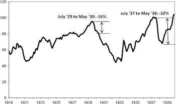
The breakdown of economic activity between the summer of 1937 and the spring of 1938 was even more dramatic than during the first phase of the Great Depression. As noted, industrial production contracted by 31 per cent, whereas its decline between the summer of 1929 and the spring of 1930 amounted to only 16 per cent (Figure 1; Freidel Reference Freidel1990). ‘In the fall of 1937’, a contemporary observer wrote, ‘industrial production began the sharpest drop on record, and by the end of the year most of the increase from the middle of 1935 had been wiped out’ (Lary Reference Lary1943, p. 197). Likewise, the fall of the Dow Jones Industrial Average was more accentuated in 1937–8, although the crash of October 1929 has been memorised as one of the worst crises in the entire history of Wall Street.Footnote ⁵

Figure 1.

Industrial production (July 1937 = 100)

Source: Federal Reserve Board. Seasonally adjusted.

The causes of the recession are not entirely clear. One view is that a combination of fiscal contraction and monetary tightening had a devastating effect on business and consumer confidence against the background of a still fragile recovery.Footnote ⁶ Another view highlights rising labour costs following the Wagner Act of 1935 which curtailed the means of employers in their actions against labour unions (Cole and Ohanian Reference Cole and Ohanian1999). In a similar vein, the BIS observed in 1939 that there can be ‘no doubt that the rise in costs of production was one of the main causes of the precipitous decline in industrial activity of the United States during the second half of 1937’ (BIS 1939, p. 10).

It is beyond the reach of this article to provide a sweeping discussion of this debate.Footnote ⁷ It is clear, however, that starting in the third quarter of 1936, monetary policy had at least some negative effect. As the rise of wholesale prices had accelerated, there was a growing sense among the Board of Governors that a new speculative bubble was in the making, similar to the one that occurred in the second half of the 1920s. The Roosevelt administration supported the Fed by issuing public statements warning of inflation. From August 1936 to May 1937, the central bank gradually increased reserve requirements for banks in order to reduce the high level of excess reserves which was considered as a potential source of future inflation.Footnote ⁸ Moreover, in December 1936, the US Treasury decided to sterilise gold inflows. Gold sterilisation led to a reduction of the money stock, and the increase of reserve requirements induced banks to curtail their financing of firms, ‘with visible effects on interest rates’ (Velde Reference Velde2009, p. 33). In 1937, fiscal policy also became less expansionary. An increase in income tax rates, the beginning of the Social Security taxation and the introduction of a tax on undistributed profits raised revenues, while an early payout of bonuses to World War I veterans before the elections of 1936 reduced spending. Altogether, government expenditure contracted by 2.3 per cent of GDP.Footnote ⁹ As John Maynard Keynes wrote to an American friend in November 1937, ‘it should have been obvious that, as soon as the Government began spending less, and as soon as the pace of improvement was somewhat moderated, a setback was entirely inevitable’.Footnote ¹⁰

As far as recovery is concerned, there is a broad scholarly consensus. In early 1938, the US authorities changed gears and initiated expansionary policies. At the end of February, the Treasury ended the gold sterilisation programme. In April, Roosevelt announced a lowering of reserve requirements and a large increase in spending. Again, the communication towards the public was loud and open. At a press conference in mid-February 1938, President Roosevelt explained ‘that achievement of permanent prosperity depends on raising general price levels to those prevailing in 1926’. The Chicago Daily Tribune, for example, ran a headline on page 1 saying ‘Hope Inflation Will Halt Depression’. Three days later, Roosevelt repeated his call for inflation.Footnote ¹¹ In the summer of 1938, the downward trend was quickly reversed. Industrial production and prices began to rise again.

Whatever the exact causes, they clearly differed from those initiating the contraction starting in the late 1920s.Footnote ¹² Nevertheless, as in 1929–30, the immediate consequences for the world economy were the same, namely a sharp reduction of world demand and world prices of raw materials. US real imports fell 50 per cent in both shocks (measured peak-to-trough in each 24-month interval).Footnote ¹³ Real global commodity prices dropped 20 per cent peak-to-trough in the 24 months of 1937–8 compared to 10 per cent (peak-to-trough) in the 24 months of 1929–30.Footnote ¹⁴ The economic situation of countries outside the US was further complicated by the reversal of capital movements. While in the last quarter of 1937 and in the first two quarters of 1938 investors exported 866 million US dollars from the US, almost the same amount of capital (733 million dollars) returned in the third and fourth quarter of 1938 when economic growth outside the US slowed down (BIS 1937/38, p. 50 and BIS 1938/39, pp. 62, 65 and 77). The reversal of capital movements was also precipitated by growing political tensions in Europe. Similarly, in 1929–30 countries outside the US had been confronted with capital outflows.

In both episodes, the Federal Reserve was required to cover 40 per cent of its notes with gold. It is clear that this covering statute did not constitute a policy constraint in the 1937 crisis – gold inflows up to this point had pushed the level of ‘active’ gold (i.e. gold beyond that needed to cover notes) to a record high of nearly 11.2 billion dollars, with the Treasury sterilising gold accumulations (Brockie Reference Brockie1950, p. 297). Regarding the 1929–30 episode, the 40 per cent cover requirement is more contentious. The New York Fed's gold holdings were at times uncomfortably near the 40 per cent minimum, which some see as limiting the Fed's room of manoeuvre, since it was not willing to jeopardise the gold standard (Eichengreen Reference Eichengreen1992, p. 325). Others argue that the Fed could have initiated an expansionary policy (including lender-of-last-resort) without upsetting the dollar's peg to gold (Hsieh and Romer Reference Hsieh and Romer2006).

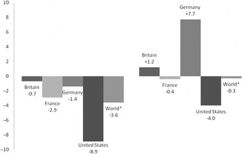
Yet, in contrast to 1930, the world economy experienced only a mild recession in 1938. Real GDP declined by 0.3 per cent against 3.6 per cent in 1930 (Figure 2).Footnote ¹⁵ Focusing on the world economy outside the US shows that real GDP in 1938 even grew slightly by 0.9 per cent against −1.7 per cent in 1930. In addition, we observe a large divergence on the country level, whereas in 1930 all major economies were entering a recession. Germany, then the second largest capitalist economy of the world (40 per cent of US GDP), grew by 7.7 per cent, whereas in 1930 it had shrunk by 1.4 per cent. Britain, the third largest capitalist economy, did better in 1938 (+1.2 per cent) than in 1930, although the recession of 1930 had not been particularly severe (−0.7 per cent). Of the large European economies only France experienced negative GDP growth (−0.4 per cent), but far less than in 1930 (−2.9 per cent).

Figure 2.

Growth of real GDP 1930 vs 1938: Britain, France, Germany, United States

Source: Maddison (2006).

Note: World* means world without Spain.

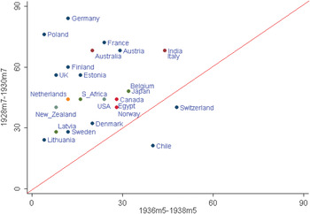
Real import data show that most countries were more reluctant to transmit the US shock to their domestic economies in 1937–8 than in 1929–30. Figure 3 reports the percentage of year-on-year declines in real imports for a 24-month period in each downturn centred on the peak of US industrial production, seasonally adjusted, by country. Only Switzerland and Chile had a higher incidence of falling real imports in the 1936–8 cycle compared to 1928–30. Conversely, because the world outside the US maintained a relatively high level of imports, American exports declined by only 7 per cent in 1938 against 27 per cent in 1930. Clearly, an accommodating stance in most large economies prevented a further contraction of world demand.

Figure 3.

Probability of annual decline in real imports in two recessions

Sources: Imports are from League of Nations, Statistical Yearbook (various years) in local currency terms, deflated by national consumer price indices from Global Financial Data.

Note: Each point reports year-on-year decline in imports during a 24-month period centred on the peak of the US industrial production index (seasonally adjusted), as a percentage of all observations (usually 24). For example, nearly 90% of monthly observations of imports for Germany in the first recession were year-on-year declines, whereas fewer than 15% of German import observations in the second recession were declines.

How can we explain that the large European economies and Japan chose to cushion the demand and price shock stemming from the collapse of US industrial production? According to the standard view in the literature, the accommodating policy reaction was due to a shift in the international monetary system. While in 1929–30 most countries were disciplined by the gold exchange standard, countries were freed from their golden fetters in 1937–8 and able to depreciate their currencies and run large fiscal deficits in order to finance their rearmament. ‘Liberated from the gold standard’, Barry Eichengreen argues, ‘other countries were not forced to match deflationary policies in the United States with their own deflationary initiatives. There was little tightening of monetary conditions outside the United States’ (Eichengreen Reference Eichengreen1992, p. 387).Footnote ¹⁶ Thanks to this freedom, Britain was able to issue a great loan to start an armament programme in 1937, a quarter of it financed by bonds, and Germany and Japan could maintain their high level of defence spending during the crisis. ‘Military spending would not have been possible had these countries still been on gold’ (p. 387).

Furthermore, instead of tightening monetary policy France and Japan let their currencies depreciate as they were losing gold to the United States. Likewise, several Latin American countries allowed their currencies to depreciate or tightened their exchange controls. This latter strategy was also chosen by some Central and Eastern European countries when their current account deficits widened. And finally, the currencies of the sterling bloc became weaker against the dollar in the second half of 1938, offsetting the deflationary effect of the US recession. Eichengreen concedes that other factors may have played a contributing role, notably the quick reversal of US policies and the stimulus of rapidly rising military spending around the world. ‘But the central factor is surely that it was no longer necessary for other countries to fight fire with fire – to meet deflation with deflation. It was only possible for them to pursue more expansionary policies than those of the United States because they had been freed from their golden fetters’ (1992, p. 389)

In the following sections we will challenge this view on three grounds. First, our exchange-rate-regime classification suggests that most countries were pegging their currencies in 1937–8 as they did in 1929–30. It is true that the Latin American countries let their currencies depreciate, but they had done the same in 1929–30, and some countries, such as Australia, even maintained their parities in contrast to 1929–30. Second, while there is no doubt that Germany was able to insulate itself thanks to tight exchange controls, most countries had rather porous capital controls in place. And third, the British rearmament programme was consistent with the rules of the gold standard.

Before proceeding, we need to treat the issue of trade openness. A stylised view of the 1930s holds that by 1937, global trade (a) was smaller than in 1929 and (b) had balkanised into semi-autarkic trading ‘blocs’, where a shock in one might not impact the rest. We acknowledge that trade volume was smaller in the 1937–8 recession than in 1929–30, but only by about 10 per cent in real terms (Eichengreen and Irwin Reference Eichengreen and Irwin1995, p. 2). Second, rather than being a novelty, the ‘balkanisation’ of 1930s trade is seen in recent literature as extending a pattern from the gold standard and even before (Ritschl and Wolf Reference Ritschl and Wolf2003; Eichengreen and Irwin Reference Eichengreen and Irwin1995).

II

Flexibility in the exchange-rate regime was not the main source of relief from the 1937–38 downturn. The BIS at the time remarked that ‘the extent to which the world's exchange position deteriorated during the year should not be exaggerated’ (BIS 1938, p. 19). The BIS referred in particular to the sterling dollar rate: ‘Over the year 1938 the exchange value of sterling declined by 6½ per cent, but even so the sterling–dollar rate was kept generally within about 4 per cent of the old par, while inside the sterling area itself no single defection occurred.’

In fact, from the outbreak of the US recession in June 1937 to June 1938 when Roosevelt had already changed course, the dollar rate of sterling remained completely stable, while overall UK exports declined by 17 per cent. It was only in the second half of 1938 that sterling depreciated 6.5 per cent against the dollar. In this period US imports increased at a fast rate. It would be hard to argue that the UK was able to cushion the US shock for the sterling area thanks to its flexible exchange rate against the dollar.

The League of Nations Yearbook 1939/1940 includes a table of 21 countries which, having left the gold standard, re-pegged their currency.Footnote ¹⁷ We see this tabulation as a contemporary acknowledgement of pegging. However, it does not go far enough. Some pegs are not reported; others are reported as adopted at dates beyond what we would consider a reasonable standard of pegging. The literature on de facto exchange-rate-regime classification offers a number of algorithms for inferring an exchange rate peg. While a review is beyond the scope of this article, a differentiating feature in the literature is the basis for judgement (Calvo and Reinhart Reference Calvo and Reinhart2002). Classification algorithms can measure exchange-rate outcomes, exchange-rate intentions, or both.Footnote ¹⁸ We adopt the outcome-based algorithm of Urban (Reference Urban2011), which is very close to that of Shambaugh (Reference Shambaugh2004). The differences between them are (1) Urban uses weekly rather than monthly observations and (2) Urban codes every observation on a rolling basis, whereas Shambaugh codes on a year-by-year basis. We code an observation as pegged if the current plus future 51 weeks lie within a ±2 percentage point band. As in Shambaugh (Reference Shambaugh2004), this is defined as the difference between the maximum and minimum of the log of the exchange rate, which must not exceed 0.04. As in Shambaugh (Reference Shambaugh2004), we accommodate a one-time peg change as consistent with a pegged regime, if the prior six months (25 weeks) and following six months exhibit less than 1 per cent weekly changes.Footnote ¹⁹ Details of our coding algorithm are available from the authors.

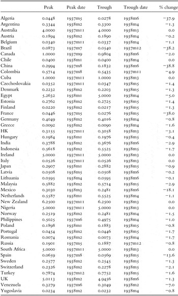
Having considered a variety of numeraires (the US dollar, UK pound sterling and French franc), it is clear that, outside the sterling bloc, most authorities are in fact pegging to gold.Footnote ²⁰ We therefore report a gold exchange rate index for each country, which tracks movement of the local currency against the dollar from 1919 up to 1932 inclusive, the French franc from 1933 to 1935 inclusive, and the dollar from 1936 till 15 August 1939. For those interested in comparing dollar-pegging to sterling-pegging in the 1930s, this gold index should be interpreted as a dollar-peg.Footnote ²¹ In Appendix 1, we report the results of our peg tests. This appendix reports the countries which pegged to sterling and those which pegged to the dollar (the gold index). There are 47 exchange-rate regimes in the dataset: Algeria, Argentina, Australia, Austria, Belgium, Brazil, Canada, Chile, China, Colombia, Cuba, Czechoslovakia, Denmark, Egypt, Estonia, Finland, France, Germany, Greece, HK, Hungary, India, Indonesia, Ireland, Italy, Japan, Latvia, Lithuania, Malaysia, Mexico, Netherlands, New Zealand, Nigeria, Norway, Philippines, Poland, Portugal, Romania, Russia, South Africa, Spain, Sweden, Switzerland, Turkey, UK, Venezuela and Yugoslavia.

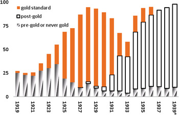
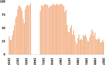
Figure 4 reports the percentage of observations coded as pegged per year, stacked by gold-convertibility. ‘Pre-gold’ are observations for regimes prior to taking up the gold standard and regimes, like Spain's and China's, which never took up the gold standard. ‘Post-gold’ are regimes which have left the gold standard.Footnote ²² The algorithm picks the appropriate peg for each 52-week period: an observation is coded ‘pegged’ if the peg criteria are met using either the gold index or the exchange rate against sterling. This is an appropriate algorithmic choice: it allows the data to speak for itself and we agree with Shambaugh (Reference Shambaugh2004) that a float is unlikely to masquerade as a peg if it meets the 52-week ±2 per cent corridor criterion.

Figure 4.

Pegged coding, percentage of annual observations, automatic numeraire

Source: Urban (2011).

Notes: *Truncated at 15/8/1939. The bars report the percentage of observations in 47 countries in 52 weeks per year which qualify as pegged on modified Shambaugh (2004) criteria. Shadings represent gold convertibility.

Floating seems to have existed only before adoption of the gold standard, mostly occurring immediately after World War I. Afterwards, there was essentially one exchange-rate regime: pegged. Gold convertibility is a separate matter. Countries which went off gold did not move to a float. The dollar's devaluation in 1933 caused much disruption, but by 1935 pegging was as common as at the peak of the gold standard.

III

It is true that capital controls were a new feature of the post-gold-standard regimes. Were they responsible for cushioning the shock emanating from the US in 1937/38? According to Gordon (Reference Gordon1941), exchange controls could be either ‘mild’ or ‘severe’, the former characterised by ‘a general supervision of applications to purchase foreign exchange’ (Gordon Reference Gordon1941, p. 62). These mild controls were adopted by the UK, Finland, USA, Belgium, Luxembourg and, until January 1937, Japan and, until May 1934, Italy. ‘Severe’ regulations ‘required the surrender of foreign balances accruing from exports’. These included Austria, Germany, Hungary, Argentina, Italy, Ecuador, Poland, Portugal, Chile, Bulgaria, Uruguay and Denmark. Gordon notes, however, that ‘outside of Germany, Italy and Japan, a substantial degree of relaxation of exchange control had been achieved’ by the mid-1930s (1941, p. 87). This suggests that capital controls for the majority of countries offered weak protection from the 1937/38 shock.

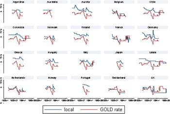
Using League of Nations coding for exchange restrictions, Obstfeld, Shambaugh and Taylor find that central banks after 1931 follow a blended Franco-US interest rate regardless of exchange-control status (Obstfeld et al. Reference Obstfeld, Shambaugh and Taylor2004, p. 18).Footnote ²³ Using a similar coding source, we break down our sample into open- and closed-capital account regimes, repeat our exchange-rate-regime classification algorithm, and explore the matter further by looking at countries singly.Footnote ²⁴Figure 5 reports gold-pegging countries' base-rate co-movement with a gold interest rate.Footnote ²⁵ Hungary's base rate, for example, follows closely on the gold interest rate irrespective of gold convertibility. Hungary suspended the gold standard in the week of 16 July 1931. Our algorithm shows it pegging the exchange rate to gold until switching to sterling in the week of 19 March 1935. Its central bank interest rate is consistent with this policy.Footnote ²⁶

Figure 5.

Central bank discount rates, gold-pegging observations

Source: Global Financial Data.

Note: The graph shows the local central bank discount rate plotted against a Franco-US hybrid interest rate (‘GOLD rate’). The plots are limited to observations for which the country is identified as pegging to a gold-hybrid exchange rate in the period 1920–39.

Cointegration tests suggested by Johansen (Reference Johansen1988), carried out in Stata, cannot reject the null hypothesis of at least one cointegrating relationship between the local discount rate and the gold interest rate for all of the gold-pegging countries except Chile, for country-specific timespans that encompass the gold standard and the post-gold period.

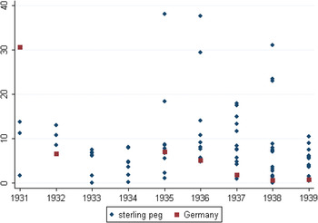
Testing capital mobility within the sterling bloc cannot be done on the basis of discount rate changes as the UK Bank rate was essentially unchanging from mid-1932, at 2 per cent. We therefore assess the openness of sterling-peg capital accounts by the volatility of their reserve holdings. If reserve volatility increases under periods of market stress, it can be inferred that reserves are being deployed to defend the peg; the greater the use of reserves, the less effective is the protection conferred by exchange controls. Figure 6 reports the coefficient of variation of reserve holdings of sterling-peg countries (as identified by our classification algorithm). The comparator is Germany, which had an unambiguously unconvertible currency. At the peak of market stress, in 1936–9, almost all sterling-bloc reserves volatility observations exceed Germany's.

Figure 6.

Reserves coefficient of variation, percentage

Source: Reserves are transcribed from Federal Reserve Bulletin (various issues).

Note: The data are truncated at 40% c.v., which excludes Germany in 1933–4.

Thus, even though some countries officially maintained exchange controls, they were not able to pursue an independent monetary policy. A case in point is Denmark. According to the classification by the League of Nations, the Danish authorities had introduced capital controls as early as 1931. Yet Denmark, as pointed out by Nurkse (Reference Nurkse1944), inflated the economy behind the protection of exchange controls, while pegging to sterling at the beginning of the decade (Nurkse Reference Nurkse1944, pp. 82–3). Because its controls were easily evaded on the current account, the decline in reserves by 1935 forced the authorities to tighten policy. In other words: it had to sacrifice policy independence in order to maintain its peg to sterling; capital controls were too weak to protect the peg.

We argue that capital controls played a minor role in cushioning the US shock in 1937–8. They were relevant for the monetary policy of Japan, Germany, and a number of Central and Eastern countries entertaining close trade relations with Germany.Footnote ²⁷ There must have been additional reasons why the world economy did not suffer from a severe recession in 1938 as it had in 1930. We now turn to the UK to explore these additional factors.

IV

The UK did not impose tight capital controls (like Germany) nor did it resort to a substantial depreciation of its currency (like France) to cushion the demand and price shock originating from the US in the second half of 1937. Accordingly, the crisis was immediately felt across the Atlantic. Between the summer of 1937 and the summer of 1938 UK industrial production declined by 23 per cent, wholesale prices dropped by more than 10 per cent, and the number of unemployed insured workers increased from 10 to 12 per cent. The reduction of industrial production in 1937–8 was almost identical to that in 1929–30. Nevertheless, the economy as a whole maintained a positive growth rate of 1.2 per cent in 1938, while in 1930 it had shrunk by 0.7 per cent.

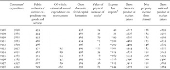
According to Eichengreen (Reference Eichengreen1992), the drop in foreign demand was compensated by a large increase in defence spending which would not have been possible under the gold standard. There is no disagreement with regard to the first part of Eichengreen's argument. As Table 1 shows, government spending in 1937 and 1938 increased by £65 million and £122 million respectively, reaching a record level of £749 million. Rising expenditure on rearmament was the main driver: in 1937 defence spending rose by £44 million and in 1938 by £73 million to a total of £262 million (all figures are in 1938 prices) (Thomas Reference Thomas1983, p. 554).Footnote ²⁸ ‘In the absence of rearmament’, writes Mark Thomas, ‘the 1937 recession would have bit harder and deeper into the gains in employment and output made over the previous five years’ (Thomas Reference Thomas1983, p. 571).

Table 1.

UK national expenditure accounts

Notes: Figures of estimated annual expenditure on rearmament from March to March, deflated by authors.

^aIncluding work in progress.

^bIncluding services and re-exports.

Source: Mitchell (Reference Mitchell1988, p. 840); data on rearmament Thomas (Reference Thomas1983, pp. 552–79).

The second part of Eichengreen's argument, however, appears to overstate the constraints of the gold standard. In 1938, defence expenditure accounted for less than 7 per cent of GNP (compared to 23 per cent in Germany), and the current account deficit deteriorated only slightly by £8 million to £55 million.Footnote ²⁹ In addition, the UK's reserve position was much better than in 1929–30. The gold reserves of the Bank of England and the Exchange Equalisation Account in 1937 were nearly six times higher than in 1931, while notes in circulation had increased by only a third. The improved relation between gold and paper money was highly relevant. Summarising the position of central banks and the international gold and capital movements, the BIS noted in spring 1939: ‘Abandonment of the gold standard has not meant the abandonment of gold either as a means of settling balances between different countries or as the usual backing for the domestic circulation according to the cover regulations of central banks.’Footnote ³⁰ The rearmament programme was clearly consistent with the rules of the gold standard.

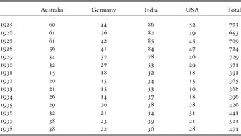
Why did the British current account deficit in 1938 not widen significantly in spite of the rearmament programme? The comparison shows that the decline of British exports was half as large in 1938 (11%) as in 1930 (22%), while imports decreased by the same percentage in both periods (11%). Given that US import demand dropped much more in 1938 (35%) than in 1930 (28%), this difference is surprising. The classification of British exports according to country, however, provides a clear answer. Two factors were crucial: the quick recovery of exports to the US and strong import demand of the UK's major trading partners, namely Germany and most members of the sterling bloc, notably Australia and India.

As for the quick reversal of the US economy, we have already described how the Roosevelt administration changed course in 1938. With US industrial production recovering in the third quarter, UK exports bounced back so that at the end of the year total exports to the US reached £28 million compared to £21 million in 1937. By contrast, in 1930, as US imports continued to decline in the second half of the year, UK exports to the US dropped from £46 to 29 million, with the difference amounting to 11 per cent of total export losses in 1930 compared to 1929 (Table 2).

Table 2.

Major export markets of the UK and total UK exports (current prices)

Source: Mitchell (2003).

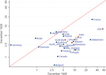
The second stabilising factor was the high level of import demand of Germany and the members of the sterling bloc, notably Australia and India (Table 2). As already mentioned, the rapid expansion of the German economy was due to an acceleration of defence spending made possible by tight capital controls. As for Australia and India, the high level of import demand was maintained in spite of high capital mobility, a pegged exchange rate and a widening gap in the trade deficit due to falling prices for raw materials. The reason for the strong import demand was the improved reserve position. Figure 7 reports the level of reserves in December preceding the peak of US industrial production in each cycle, as a ratio to the average monthly import bill. Both Australia and India had significantly improved their reserve position between 1928 and 1936.

Figure 7.

Reserves, months of import coverage

Source: League of Nations, Statistical Yearbook (various years).

Note: Each data point reports the number of months of imports covered by reserves, based on the average monthly import bill of the year. The scale is logarithmic.

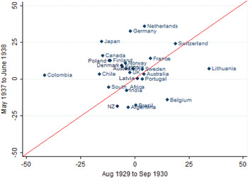
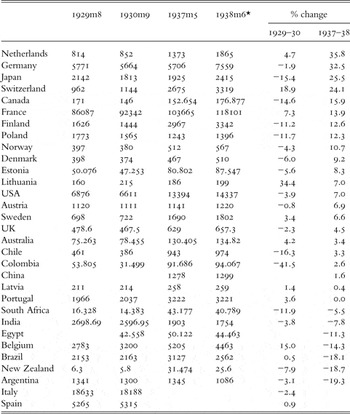
The support for aggregate demand in the 1937–8 downturn reflects a variety of sources – in some cases, as noted, it includes sustained import demand among trade partners. In other cases, central banks actively acquired domestic assets to keep base money supply from contracting, or indeed to expand it. Figure 8 reports the expansion of base money during the 13-month 1937–8 US downturn and the 13 months beginning with the US 1929–33 downturn. It is important to compare like with like in terms of the time period because part of our argument is that the brevity of the 1937–8 downturn was part of the reason for the global resilience, vis-à-vis the much longer 1929–33 US downturn.

Figure 8.

Expansion of base money over two recessions

Sources: Federal Reserve Bulletin, League of Nations Monthly Bulletin of Statistics, Economist.

Note: Data points are reported in Appendix 2.

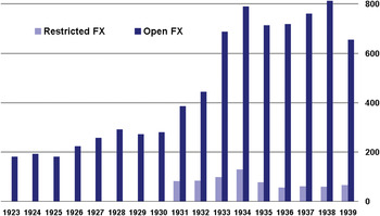
International liquidity was simply greatly improved at the time of the 1937–8 downturn compared to 1929–30. This is clear in terms of import cover, as in Figure 7, and it is clear in terms of absolute quantity of global reserves, measured in constant terms, as in Figure 9, which distinguishes between countries that had restrictive capital-account convertibility and those with open capital-account convertibility.Footnote ³¹

Figure 9.

Mean reserves in millions of 1928 US dollars

Source: Urban (2011).

Note: The y-axis is reserves of gold and foreign exchange in 1928 US dollar millions. Bars are mean value at end-year for a panel of 31 countries, excluding the USA. The figure for 1939 is August.

The importance of increased reserves was highlighted by a contemporary study by the US Department of Commerce (Lary Reference Lary1943). This study also pointed out that exchange rate flexibility mattered only for some Latin American countries, but not for most European countries:

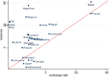
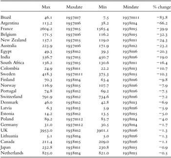
Figure 10 reports the peak-to-trough decline in reserves in the US downturn interval (May 1937 – June 1938) for our sample of 28 countries with balance-sheet data. These are compared with the extent of the depreciation of the exchange rate over the same interval.

Figure 10.

Percentage decline in reserves and exchange rate (absolute value), peak-to-trough during May 1937 – June 1938

Sources: Federal Reserve Bulletin, League of Nations Monthly Bulletin of Statistics, Economist, Global Financial Data.

Notes: Peak/trough dates and data points are reported in Appendix 2. Reserves are in US dollar terms, converted from local currency terms with bilateral US dollar exchange rate from Global Financial Data. The exchange rate is the percentage change in the bilateral rate against the US dollar, in USD/local currency terms.

Our argument is that a higher degree of international liquidity among central banks (i.e. larger levels of reserves) allowed countries to weather the 1937–38 US recession without inducing their own contractions, as would be required under the conditions of a currency peg and (relatively) open international accounts. It bears noting that this point holds regardless of the status of statutory requirements for minimum gold backing of base money; these only shift the level of reserves needed to defend the peg.Footnote ³²

V

Why was the global downturn following the sharp US recession of 1937–8 much milder than in 1930? This article discussed the conventional explanation focusing on the new international monetary environment allowing more exchange rate flexibility, capital controls and thus more room for fiscal deficits. We come to the conclusion that these are not the main factors behind the cushioning of the economic shock coming from the US. First, exchange rate flexibility was confined to a rather small group of countries. Second, capital controls were much less tight than official classifications suggest. And third, the fiscal room of manoeuvre of the UK government was large enough to reconcile the rearmament programme with a stable exchange rate against the US dollar.

This finding concurs with several recent studies on the post-1931 international monetary system (Straumann and Woitek Reference Straumann and Woitek2009; Urban Reference Urban2011; Wandschneider and Wolf Reference Wandschneider and Wolf2010; Wolf Reference Wolf2010). They all point out that the break with the gold exchange standard of the 1920s was less abrupt than usually assumed. Most countries, in particular the smaller ones, maintained a fixed exchange rate against their main trading partners, thus being subject to the same rules the gold exchange standard had imposed upon them. It would be wrong to claim that there was no change at all. But the fact that enhanced reserve positions made a crucial difference between the downturns of 1930 and 1938 suggests that currency devaluation – not fundamental regime change – was the major monetary change of the 1930s.

From a longer-term perspective, the 1930s international monetary system evolved in a way that connected the interwar gold standard to the Bretton Woods system (1947–71). It was a de facto arrangement of what would be made de jure at Bretton Woods. We favour this viewpoint over the alternative that the 1930s was a period of floating exchange rates anticipating the modern, post-Bretton Woods period (Eichengreen Reference Eichengreen1992, p. 395). We are not the first to cast the 1930s system as a forerunner of Bretton Woods. Mundell describes a dollar-based international order which begins from stabilisation on the $35 gold price in 1934 and lasts until 1971 (Mundell Reference Mundell and Acheson1972, p. 96). Eichengreen and others see traces of the Bretton Woods system from the signing of the Tripartite Agreement in 1936 (Eichengreen Reference Eichengreen1990, p. 151). What we add is a quantification of that similarity. Applying our weekly rolling variant of the Shambaugh (Reference Shambaugh2004) algorithm to a longer span of history helps illustrate how similar the 1930s are to the Bretton Woods system (Figure 11).

Figure 11.

Pegged regimes, percentage of total annual observations

Source: Urban (2011). Compiled from weekly observations of 47 countries with automatic numeraire selection.

Flexible exchange rate regimes did not arrive until the early 1970s when the Bretton Woods system collapsed. Comparative studies on the exchange rate choices of small European states even suggest that only with the crisis of the European monetary system in 1992/93 did the idea that small states were able to manage floating exchange rates gain currency. Before, policymakers had been convinced that small open economies needed fixed exchange rates as a precondition for stable trade relations and price stability (Straumann Reference Straumann2010). Lastly, our story is a case of history repeating itself. Just as the emerging markets and periphery economies of the interwar years survived the 1937–8 shock through a strong reserves position, so too have the emerging markets of today weathered the 2007–8 financial crisis.