1. Introduction
Over the past decades, a large amount of experimental and numerical work has been carried out to understand and predict complex granular flow behaviours. Laboratory experiment is an essential approach to observe granular flows in controlled conditions, e.g. the flow down an inclined chute (Savage & Lun Reference Savage and Lun1988; Pouliquen Reference Pouliquen1999; Gollin et al. Reference Gollin, Brevis, Bowman and Shepley2017), the granular column collapse (Balmforth & Kerswell Reference Balmforth and Kerswell2005; Lajeunesse, Monnier & Homsy Reference Lajeunesse, Monnier and Homsy2005; Lube et al. Reference Lube, Huppert, Sparks and Freundt2005) and the flow in a rotating drum (Ristow Reference Ristow1996; Mellmann Reference Mellmann2001; Liu, Specht & Mellmann Reference Liu, Specht and Mellmann2005). Meanwhile, some key flow characteristics, e.g. the shear rate close to the boundary and the local pressure level, are still difficult to measure in experiments, but are accessible directly in numerical simulations. There are mainly two modelling approaches. In discrete methods, particles in granular flows are represented by individual elements that can interact with each other through contact models (Cundall & Strack Reference Cundall and Strack1979). In continuum methods, the granular materials are treated as a fluid, which allows the modelling of granular flows using a large variety of hydrodynamic approaches (Lacaze & Kerswell Reference Lacaze and Kerswell2009; Lagrée, Staron & Popinet Reference Lagrée, Staron and Popinet2011; Chauchat & Médale Reference Chauchat and Médale2014; Franci & Cremonesi Reference Franci and Cremonesi2019; Yang et al. Reference Yang, Yang, Jing, Kwok and Sobral2023). The continuum approaches enable the possibility of large-scale simulations at an acceptable computational cost, but require a thorough understanding of the granular flow physics, including the constitutive relations for the stresses and the boundary conditions, which remain the major challenges.
Great efforts have been made to define proper constitutive relations of granular flows across different flow regimes, and successful outcomes have been achieved to capture the solid-like, liquid-like and gas-like behaviours (Campbell Reference Campbell1990; Johnson, Nott & Jackson Reference Johnson, Nott and Jackson1990; Goldhirsch Reference Goldhirsch2003; Midi Reference Midi2004; Jop, Forterre & Pouliquen Reference Jop, Forterre and Pouliquen2006). Meanwhile, relatively less work has been devoted to develop proper boundary conditions for granular flows, especially in the dense flow regime in which particles undergo enduring contacts, and energy dissipation is governed by friction (Artoni, Santomaso & Canu Reference Artoni, Santomaso and Canu2009; Artoni et al. Reference Artoni, Santomaso, Go’ and Canu2012). Indeed, simplified and common boundary conditions in computational fluid dynamics (CFD), i.e. no-slip and free-slip, are often adopted to describe rough and smooth walls (Lagrée et al. Reference Lagrée, Staron and Popinet2011; Yang et al. Reference Yang, Yang, Jing, Kwok and Sobral2023). Nevertheless, the frictional nature of dense granular flows and their interactions with solid boundaries usually produce a complex stick–slip behaviour that is neither no-slip nor free-slip (Nasuno et al. Reference Nasuno, Kudrolli, Bak and Gollub1998; Artoni et al. Reference Artoni, Santomaso and Canu2009, Reference Artoni, Santomaso, Go’ and Canu2012; Jing et al. Reference Jing, Kwok, Leung and Sobral2016). It is worth mentioning that although the boundary may cover only a small percentage of the whole simulation domain, the effect of a boundary condition is rather significant and is no less important than the rheology of the flow. In fact, it is the boundary condition that often determines the overall convergence rate and shapes all kinds of CFD simulations.
Recently, the lattice Boltzmann method (LBM) has been applied successfully as an accurate and efficient numerical tool to model dense granular flows (Yang et al. Reference Yang, Yang, Jing, Kwok and Sobral2023). Instead of solving directly for the macroscopic quantities, i.e. velocity and pressure – as is normally the case in conventional CFD approaches based on Navier–Stokes equations using finite difference or other discretization schemes – the LBM solves hydrodynamic problems via a set of density distribution functions streaming and colliding on a regular lattice (Chen & Doolen Reference Chen and Doolen1998). The kinetic heritage of the LBM encourages boundary conditions to be formulated based on the bounce-back and the specular reflection (mirror-like) of density distribution functions for the no-slip and free-slip boundary conditions, respectively (Reis Reference Reis2020). This heuristic way of handling boundary conditions is simple and straightforward, which promotes the use of the LBM for simulating fluid flows in complex geometries, such as flow through porous media (Aharonov & Rothman Reference Aharonov and Rothman1993; Dong, Yan & Li Reference Dong, Yan and Li2011).
Another popular application of the LBM is to simulate fluid flows in microchannels and rarefied gas flows, in which the continuity assumption breaks down and there exist slip velocities at boundaries (Chai et al. Reference Chai, Guo, Zheng and Shi2008; Wang et al. Reference Wang, Chai, Hou, Chen and Xu2018). In such conditions, the Navier slip model that linearly correlates the slip velocity  $u_w$ with the shear rate
 $\dot {\gamma }_w$ near the boundary is adopted commonly, namely
 $u_w=l_s \dot {\gamma }_w$, where
 $l_s$ is the so-called slip length. In the LBM, this partial-slip boundary condition is implemented simply at the mesoscopic scale that linearly combines the bounce-back and the specular reflection schemes (Succi Reference Succi2002). The amount of boundary slip is determined by a single constant
 $r$, sometimes called the molecular slip coefficient (Švec & Skoček Reference Švec and Skoček2013). Generally, the molecular slip coefficient
 $r$ varies between 0 and 1, and the boundary slip gradually attenuates as
 $r$ increases. However, the boundary slip for the flow of granular materials occurs only beyond a critical threshold, which depends on the wall roughness (Jing et al. Reference Jing, Kwok, Leung and Sobral2016), and such a yielding criterion is still absent in the currently available slip length models.
Despite the successful applications of the LBM for different fluid flow problems with complex boundary conditions, to our best knowledge, there seems to be no existing boundary condition characterized by friction, which limits the capability of the LBM for dense granular flow simulations. The goal of this study is to develop a frictional boundary condition for the LBM so that the shear stress at the boundary is limited by the Coulomb friction. We are aware of the more advanced boundary conditions that derive from the Navier slip model (Artoni et al. Reference Artoni, Santomaso and Canu2009, Reference Artoni, Santomaso, Go’ and Canu2012; Artoni & Santomaso Reference Artoni and Santomaso2014). However, as a first attempt, we focus on the simple Coulomb friction boundary condition, which is characterized by a constant friction coefficient. Similar boundary conditions have been implemented in other numerical methods (Wu, Hill & Yu Reference Wu, Hill and Yu2007; Domnik & Pudasaini Reference Domnik and Pudasaini2012), and have been proved to be essential components to reproduce the complex stick-slip behaviour at the boundary. Our results also show that this simplified boundary condition, as a direct derivation from the frictional nature of dense granular flows, can improve drastically the predictability of continuum models for transient flow problems, such as the granular column collapse.
This paper is organized as follows. Section 2 presents the LBM, with particular focus on the free-surface tracking and the granular flow rheology. Detailed implementation of the newly proposed frictional boundary condition is also introduced. A unique plane Couette flow with a frictional and stationary bottom wall is simulated to validate the numerical model in § 3. Then LBM simulation of a granular column collapse over a horizontal bottom plane is performed in § 4, and the model parameters, including the wall friction coefficient, are calibrated against the discrete element results. The same model parameters after calibration are employed in § 5 for the LBM simulation of granular column collapses with different aspect ratios and on a slope. Conclusions are drawn in § 6.
2. Model formulation
2.1. Lattice Boltzmann method
2.1.1. The D2Q9 Bhatnagar–Gross–Krook model
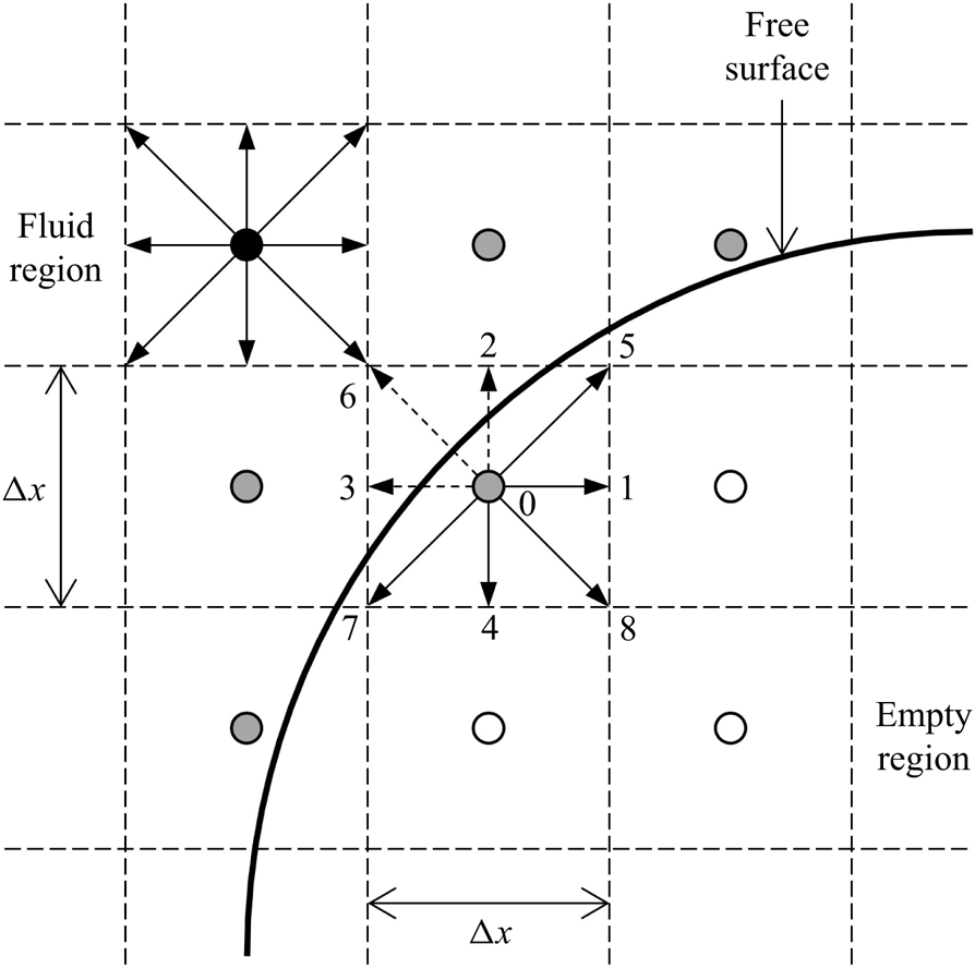
Since the LBM is based on the kinetic theory of gases, the method deals with mesoscopic density distribution functions, rather than macroscopic flow quantities, such as velocity and pressure (Chen & Doolen Reference Chen and Doolen1998). The density distribution functions determine physically the amount of fluid moving in space with certain velocities. To solve the Boltzmann equation numerically, the two-dimensional space is commonly discretized into square fluid cells forming a uniform Cartesian grid. Figure 1 shows a sketch of the D2Q9 lattice structure with 9 discrete velocities (including one at rest) in two dimensions (Qian, D'Humières & Lallemand Reference Qian, D'Humières and Lallemand1992). The propagation of density distribution functions to the neighbour fluid cells is allowed only along the orthogonal and diagonal directions, by following the lattice Boltzmann equation. Considering a Bhatnagar–Gross–Krook approximation and a body force term for the collision operator, we can write the lattice Boltzmann equation as (He et al. Reference He, Zou, Luo and Dembo1997)
 \begin{equation} f_i(\boldsymbol{x}+\boldsymbol{c}_i\,\Delta t, t+\Delta t)-f_i(\boldsymbol{x}, t) ={-}\frac{1}{\tau}\,[ f_i(\boldsymbol{x}, t)-f_i^{eq}(\boldsymbol{x}, t) ] + w_i\, \frac{\boldsymbol{c}_i \boldsymbol{\cdot} \boldsymbol{F}}{c_s^2}, \end{equation}
where the density distribution function  $f_i(\boldsymbol {x},t)$ represents the amount of fluid positioned at
 $\boldsymbol {x}$ at time
 $t$ moving with velocity
 $c_i$ along the
 $i$th direction at each lattice node, and
 $i$ varies from 0 to 8 for the D2Q9 model (see figure 1). The time step is denoted by
 $\Delta t$. The body force density is denoted by
 $\boldsymbol {F}=\rho \boldsymbol {g}$, where
 $\rho$ is the fluid density and
 $\boldsymbol {g}$ is commonly the gravitational acceleration. The dimensionless relaxation time is denoted by
 $\tau$, which determines physically how fast the density distribution function recovers the equilibrium state
 $f_i^{eq}(\boldsymbol {x},t)$. The equilibrium distribution function depends on the macroscopic fluid density
 $\rho$ and velocity
 $\boldsymbol {u}$, which can be expressed as (Qian et al. Reference Qian, D'Humières and Lallemand1992)
 \begin{equation} f_i^{eq} = w_i \rho \left[ 1+\frac{\boldsymbol{c}_i \boldsymbol{\cdot} \boldsymbol{u}}{c_s^2}+\frac{(\boldsymbol{c}_i \boldsymbol{\cdot} \boldsymbol{u})^2}{2c_s^4}-\frac{\boldsymbol{u}^2}{2c_s^2} \right], \end{equation}
where  $w_i$ is the weighting coefficient, and
 $c_s$ is the speed of sound. For the D2Q9 model,
 $w_0=4/9$,
 $w_i=1/9$ for
 $i=1\unicode{x2013}4$ (orthogonal directions),
 $w_i=1/36$ for
 $i=5\unicode{x2013}8$ (diagonal directions), and
 $c_s=1/\sqrt {3}$ in lattice units (Qian et al. Reference Qian, D'Humières and Lallemand1992). The macroscopic fluid density
 $\rho$ and velocity
 $\boldsymbol {u}$ can be reconstructed from the density distribution functions according to the conservation of mass and momentum:
 $$\begin{gather} \rho = \sum_{i=0}^8 f_i, \end{gather}$$
 $$\begin{gather}\rho \boldsymbol{u} = \sum_{i=0}^8 \boldsymbol{c}_i f_i. \end{gather}$$
Sketch of the D2Q9 lattice structure. The black, grey and white circles represent the fluid, interface and empty nodes, respectively. The dashed lines stand for the cell boundaries. The solid line depicts the free surface going through the interface cells.

A multiscale Chapman–Enskog expansion can be performed on (2.1) (He & Luo Reference He and Luo1997) to obtain the conventional Navier–Stokes equation with a relation between the relaxation time  $\tau$ and the fluid kinematic viscosity
 $\nu$ given by
 \begin{equation} \nu = c_s^2 \left( \tau-\tfrac{1}{2} \right). \end{equation}
For isothermal problems, the local pressure  $p$ is related to the fluid density by the equation of state (He & Luo Reference He and Luo1997)
 \begin{equation} p = c_s^2 \rho. \end{equation}
2.1.2. Free-surface tracking
The problem of dense granular flows, such as the granular column collapse (see § 4), usually involves a dynamic evolution of the particle–air interface, i.e. the free surface. In this study, a single-phase free-surface tracking algorithm originally proposed to optimize the production process of metal foams is adopted (Körner et al. Reference Körner, Thies, Hofmann, Thürey and Rüde2005). Different from the normal LBM, in which there exist only fluid and boundary nodes, the free-surface model introduces two additional types of lattice nodes: the interface node and the empty node (see figure 1). Each lattice node is located at the centre of a lattice cell and is associated with the corresponding cell type. In LBM calculations, the different cell types are distinguished by a single parameter, i.e. the fluid volume fraction of a lattice cell  $\varepsilon$, which is given by
 \begin{equation} \varepsilon = \frac{m}{\rho}, \end{equation}
where  $m$ is the mass of fluid contained in a cell, and the fluid density
 $\rho$ is calculated using (2.3a). Note that the physical lengths are non-dimensionalized by the lattice spacing
 $\Delta x$ before actual calculation. Therefore, the volume of a lattice cell becomes 1 in lattice units, and (2.6) essentially gives a dimensionless fluid volume fraction
 $\varepsilon$, instead of a result in units of volume. The value of
 $\varepsilon$ ranges from 0 to 1:
 $\varepsilon =0$ for empty cells,
 $\varepsilon \in (0, 1)$ for interface cells, and
 $\varepsilon =1$ for fluid cells.
The dynamic evolution of the free surface is achieved by the conversion of interface cells to fluid or empty cells, depending on the fluid volume fraction  $\varepsilon$. It requires the exact mass exchange between adjacent cells during the propagation of density distribution functions, which can be calculated as
 \begin{equation} \Delta m_i(\boldsymbol{x}, t+\Delta t) = [\,f_{{-}i}(\boldsymbol{x}+\boldsymbol{c}_i \Delta t, t)-f_i(\boldsymbol{x}, t) ]\,\frac{\varepsilon(\boldsymbol{x}+\boldsymbol{c}_i \Delta t, t)+\varepsilon(\boldsymbol{x}, t)}{2}, \end{equation}
in which the averaged fluid fraction has been used to approximate the contact area between two adjacent cells. The subscript  $-i$ denotes the direction opposite to
 $i$. The new mass value is obtained by adding the mass flux in all directions (except the one at rest) to the current value:
 \begin{equation} m(\boldsymbol{x}, t+\Delta t) = m(\boldsymbol{x}, t)+\sum_{i=1}^8 \Delta m_i(\boldsymbol{x}, t+\Delta t). \end{equation}
Note that (2.7) is symmetric, meaning that the mass of fluid leaving one cell has to enter another cell, and the total mass is conserved up to machine precision. Another advantage of the single-phase free-surface model is that the empty cells are never accessed during actual calculations. Compared to the conventional volume-of-fluid method in CFD that solves both the fluid and the empty (i.e. air) phases (Lagrée et al. Reference Lagrée, Staron and Popinet2011), the single-phase model is computationally efficient and largely saves computer memory (Yang et al. Reference Yang, Yang, Jing, Kwok and Sobral2023). Meanwhile, a proper free-surface boundary condition is required to reconstruct the unknown density distribution functions streaming from the empty cells to the interface cells; see the arrows with dashed lines in figure 1. It is assumed that the air density is  $\rho _A=1$ (equivalent to zero gauge pressure) and that the air shares the same velocity
 $\boldsymbol {u}$ with the fluid at the free surface, so that the unknown density distribution functions can be calculated via the bounce-back of the non-equilibrium part:
 \begin{equation} f_{{-}i}(\boldsymbol{x}, t+\Delta t) = f_i^{eq}(\rho_A, \boldsymbol{u})+f_{{-}i}^{eq}(\rho_A, \boldsymbol{u})-f_i(\boldsymbol{x}, t). \end{equation}
A full set of density distribution functions coming from the empty region for all interface cells (including the ones that interact with the solid boundary, e.g. at the tip of a flow) can be obtained by applying (2.9) to all directions with empty neighbour cells. In this way, any physics related to the presence of three phases, e.g. the surface tension, is ignored, and we assume that those effects are negligible in our problem. Also, the propagation of flow front in CFD-like continuum simulations requires an additional treatment to solve the so-called moving contact line problem (Liu et al. Reference Liu, Balmforth, Hormozi and Hewitt2016), which is not present in the LBM due to its particulate nature. Note that only the key equations for the mass exchange and the free-surface boundary condition are presented here, and further details about cell type conversion are available from Körner et al. (Reference Körner, Thies, Hofmann, Thürey and Rüde2005) and Thürey & Rüde (Reference Thürey and Rüde2009).
2.1.3. Granular flow rheology
To model dense granular flows, a special rheology has to be applied. One remarkable finding of previous research is that granular materials flow like viscoplastic fluids, which have a solid-like behaviour at low shear stress, and flow like liquid at high shear stress (Midi Reference Midi2004; Jop et al. Reference Jop, Forterre and Pouliquen2006; Lacaze & Kerswell Reference Lacaze and Kerswell2009). In our recent work, the most widely adopted  $\mu (I)$-rheology for dense granular flows is implemented successfully using the LBM, and the resulting framework is called LBGrain (Yang et al. Reference Yang, Yang, Jing, Kwok and Sobral2023). The
 $\mu (I)$-rheology can be regarded as an extended Coulomb friction law with a varying friction coefficient
 $\mu$ that depends on the dimensionless inertial number
 $I$ (Midi Reference Midi2004; Jop et al. Reference Jop, Forterre and Pouliquen2006). So we have
 \begin{equation} \mu(I) = \frac{\sigma}{p}, \quad \text{with} \ I = \frac{\dot{\gamma} d_p}{\sqrt{p/\rho_p}}, \end{equation}
where  $\dot {\gamma }$ is the shear rate,
 $d_p$ is the particle diameter, and
 $\rho _p$ is the particle density. Note that here we use
 $\sigma$ to denote the shear stress, since the commonly used symbol
 $\tau$ has been assigned to denote the relaxation time in the LBM. Previous experiments and discrete element simulations have demonstrated that the friction coefficient
 $\mu$ is an increasing function of the inertial number
 $I$ (Midi Reference Midi2004; Jop et al. Reference Jop, Forterre and Pouliquen2006; Lacaze & Kerswell Reference Lacaze and Kerswell2009), which can be written as
 \begin{equation} \mu(I) = \mu_s+\frac{\mu_d-\mu_s}{I_0/I+1}, \end{equation}
where  $\mu _s$,
 $\mu _d$ and
 $I_0$ are model constants that depend on the frictional material properties. For viscous fluids, the shear stress is proportional to the local shear rate, i.e.
 $\sigma = \eta \dot {\gamma }$, where
 $\eta$ is the proportionality constant and is normally called the dynamic viscosity. Using the Coulomb friction law for the shear stress, we can get an apparent fluid viscosity
 $\eta _{app}$ that depends on the local shear rate and the local pressure level:
 \begin{equation} \eta_{app}(\dot{\gamma}, p) = \frac{\mu(I)\,p}{\dot{\gamma}} = \frac{p \mu_s}{\dot{\gamma}}+\frac{p (\mu_d-\mu_s)}{I_0\sqrt{p/\rho_p}+d_p\dot{\gamma}}\,d_p. \end{equation}
However, (2.12) is ill-defined at zero shear rate, in which case the apparent viscosity becomes infinitely large. This is encountered commonly when a static initial condition is applied. The solution is to adopt a regularization method so that the apparent viscosity converges to a finite large value as the shear rate vanishes. Here, we use the Papanastasiou method, and (2.12) is modified as (Chauchat & Médale Reference Chauchat and Médale2014; Franci & Cremonesi Reference Franci and Cremonesi2019)
 \begin{equation} \eta_{app} = \frac{p \mu_s}{\dot{\gamma}}\,( 1-{\rm e}^{-{\dot{\gamma}}/{\lambda}})+\frac{p (\mu_d-\mu_s)}{I_0\sqrt{p/\rho_p}+d_p\dot{\gamma}}\,d_p, \end{equation}
where  $\lambda$ is the regularization parameter. In general, a smaller
 $\lambda$ value yields a better approximation of the ideal rheology (Yang et al. Reference Yang, Yang, Jing, Kwok and Sobral2023). Note that only the first term on the right-hand side of (2.13) has been regularized, and the second term still diverges when both the pressure
 $p$ and the shear rate
 $\dot {\gamma }$ are equal to zero. Therefore, a small pressure,
 $\Delta p = \rho g d_p$, corresponding to one layer of particles below the free surface, is added to the local pressure if
 $p = 0$ and
 $\dot {\gamma } = 0$ simultaneously, to avoid division by zero.
Within the lattice Boltzmann framework, the fluid viscosity is related directly to the relaxation time through (2.4), i.e.  $\eta = \rho \nu = \rho c_s^2 (\tau -0.5)$. To model dense granular flows, the fluid viscosity in (2.4) is replaced by the apparent value given by (2.13), so that an effective local relaxation time is obtained:
 \begin{equation} \tau_{eff} = \frac{\eta_{app}}{\rho c_s^2}+\frac{1}{2}. \end{equation}
The lattice Boltzmann modelling of dense granular flows is achieved by substituting the effective relaxation time  $\tau _{eff}$ into (2.1) for the collision operator. Similarly to the apparent viscosity, the effective relaxation time in the LBM now depends on the local shear rate and the local pressure level, which are updated continuously during the calculation. The proposed numerical framework for lattice Boltzmann modelling of dense granular flows (i.e. LBGrain) has been validated against analytical solutions of simple flow conditions and discrete element simulations, and has been proved to be computationally accurate and efficient (Yang et al. Reference Yang, Yang, Jing, Kwok and Sobral2023).
2.2. Frictional boundary condition
Defining appropriate boundary conditions is as important as applying proper rheologies when solving hydrodynamic problems. In the LBM, there are mainly two ways to implement various boundary conditions. On one hand, boundary conditions can be defined phenomenologically. Typical examples are the bounce-back scheme for no-slip, the specular reflection scheme for free-slip, and the direct propagation of density distribution functions across boundaries in the same direction for the periodic boundary condition (Chen, Martínez & Mei Reference Chen, Martínez and Mei1996). On the other hand, boundary conditions can also be defined hydrodynamically. The unknown density distribution functions propagating from the boundary to the fluid domain are reconstructed based on their relationships with the macroscopic flow quantities (Chen et al. Reference Chen, Martínez and Mei1996; Zou & He Reference Zou and He1997); see (2.3) and (2.5), which are normally well defined at the boundaries.
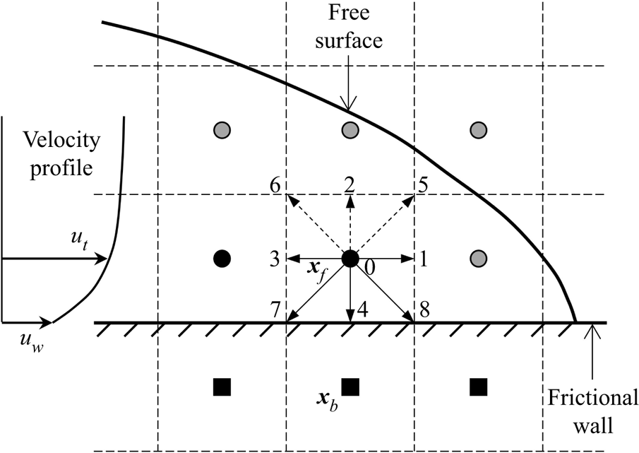
In this study, we propose a novel boundary condition governed by the Coulomb friction law for the LBM. Wall slip takes place provided that the wall shear stress, i.e. the product of the shear rate and the flow viscosity at the boundary, exceeds a critical threshold set by the Coulomb friction. The way of implementing the frictional boundary condition is a hybrid method that combines both the phenomenological and the hydrodynamic approaches. Figure 2 shows a sketch of the lattice grid near a frictional wall, which sits halfway between the fluid (or interface) nodes and the frictional nodes. In this particular case, the density distribution functions  $f_2$,
 $f_5$ and
 $f_6$ have to be constructed based on the frictional boundary condition. First, the shear rate at the wall is estimated by the finite difference method,
 $\dot {\gamma }_w = 2(u_t-u_w)$, where
 $u_t$ and
 $u_w$ denote the tangential components of the velocity at the wall and at the fluid (or interface) node just next to the wall. Second, the maximum allowable shear rate is calculated based on the Coulomb friction law:
 \begin{equation} \dot{\gamma}_{max} =\begin{cases} \mu_w p / \eta_{app} & \text{if}\ p > 0,\\ 0 & \text{if}\ p \leq 0, \end{cases} \end{equation}
where  $\mu _w$ is the constant wall friction coefficient, and
 $p$ and
 $\eta _{app}$ are estimated at the fluid or interface node near the wall. Third, the wall slip velocity
 $u_w$ is adjusted according to the flow kinematics. If
 $\dot {\gamma }_w > \dot {\gamma }_{max}$, then the upper limit set by the Coulomb friction is reached and partial-slip takes place at the wall. Then the new wall slip velocity is calculated as
 \begin{equation} u_w = u_t - 0.5 \dot{\gamma}_{max}\,\frac{\dot{\gamma}_w}{|\dot{\gamma}_w|}. \end{equation}
Sketch of the velocity profile and the lattice grid near a frictional wall. The black squares represent the frictional nodes. The symbols  $\boldsymbol {x}_b$ and
 $\boldsymbol {x}_f$ denote the locations of the frictional node and the fluid (or interface) node next to the frictional wall, respectively. The frictional wall sits halfway between the fluid (or interface) nodes and the frictional nodes, so it overlaps with the cell boundaries. See the caption of figure 1 for other notations.

When  $\dot {\gamma }_w \leq \dot {\gamma }_{max}$ and there exists a finite wall slip velocity, i.e.
 $u_w \neq 0$, the Coulomb friction is still fully active. Then the wall slip velocity is updated as
 \begin{equation} u_w = u_t - 0.5 \dot{\gamma}_{max}\,\frac{u_t}{|u_t|}. \end{equation}
The minus signs in (2.16) and (2.17) indicate that the frictional force always acts in the opposite flow direction. Also, the frictional force can only provide resistance to the flow, therefore no change of sign for the wall slip velocity  $u_w$ is allowed in (2.17), and the wall slip velocity will be set to 0 when it happens. If
 $\dot {\gamma }_w \leq \dot {\gamma }_{max}$ and
 $u_w = 0$, then the slip criterion set by the Coulomb friction law is not reached and the wall slip velocity
 $u_w$ will remain at 0, recovering the no-slip boundary condition.
Finally, a modified bounce-back scheme is applied to constructed the unknown density distribution functions, e.g.  $f_2$,
 $f_5$ and
 $f_6$ in figure 2, considering the updated wall slip velocity (Ladd Reference Ladd1994):
 \begin{equation} f_{{-}i}(\boldsymbol{x}_f, t+\Delta t) = f_i(\boldsymbol{x}_f, t) - 2w_i \rho\,\frac{\boldsymbol{c}_i \boldsymbol{\cdot} \boldsymbol{u}_w}{c_s^2}, \end{equation}
where  $\boldsymbol {x}_f$ is the location of the fluid or interface node next to the frictional wall.
There are several characteristics of the proposed frictional boundary condition that are worth mentioning. The updates of the wall slip velocity and the density distribution functions are carried out in a progressive manner. This means that the constraint posed by the Coulomb friction law is well considered by the flow kinematics at the boundary, so that the whole problem is translated into the determination of the correct wall slip velocity. Then the conventional moving wall boundary condition, i.e. (2.18), can be applied directly, which facilitates an easy implementation into any available LBM code. Also, the modified bounce-back scheme can be extended easily to three-dimensional conditions. Furthermore, since the same wall slip velocity  $\boldsymbol {u}_w$ is used in (2.18) to construct the unknown density distribution functions for a certain fluid or interface node, the quantities added to and subtracted from the fluid domain are identical, at least for the flat walls considered in this study. As a result, the mass of the whole system is well conserved, which is essential for problems when a dynamic free surface is present.
3. Validation of the frictional boundary condition
3.1. Plane Couette flow with a frictional and stationary bottom wall
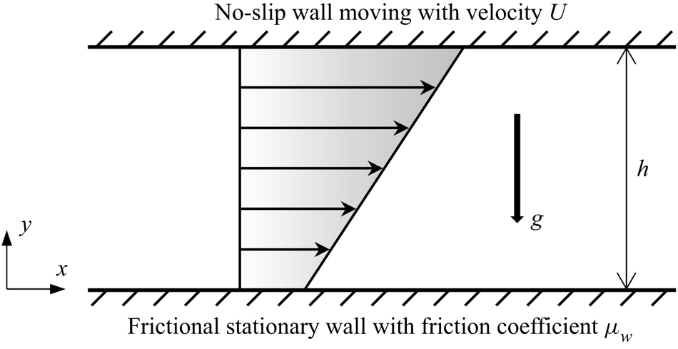
To validate the frictional boundary condition, we design a unique plane Couette flow as shown in figure 3. In this validation section, we focus on the steady flow of a Newtonian fluid between two infinite parallel walls placed at a distance  $h$ apart. The flow is driven by the upper wall with a constant velocity
 $U$, and it is assumed that the no-slip boundary condition holds so that the fluid shares the same velocity with the upper wall, i.e.
 $u = U$ at
 $y = h$. The lower wall is still kept stationary but becomes frictional with a predefined friction coefficient
 $\mu _w$. To facilitate a finite frictional resistance at the lower wall, a positive pressure has to be applied; see (2.15). Therefore, the flow is subjected to a gravity field with a magnitude equal to
 $g$ pointing downwards, which is normally ignored when solving the conventional plane Couette flow problem. The frictional bottom wall results in a boundary condition characterized by a dynamic shear stress, which depends on the friction coefficient and the local pressure level. The validity of the frictional boundary condition combined with the granular flow rheology and the free surface will be tested against discrete element simulations regarding the transient granular column collapse in §§ 4 and 5.
Sketch of the steady plane Couette flow. The flow is driven by the upper wall with a constant velocity  $U$ moving in the positive
 $x$-direction. The lower wall is stationary with a constant friction coefficient
 $\mu _w$ that permits wall slip.

There are mainly two reasons why we choose plane Couette flow for the validation of the frictional boundary condition. First, this simple shear configuration has been applied widely in physical experiments and numerical simulations to investigate the rheology of all kinds of fluid flows, including dense granular flows (Midi Reference Midi2004). Second, an analytical solution can be derived easily to measure the accuracy and the convergence rate of the proposed frictional boundary condition. For a certain driving velocity of the upper wall, when the friction coefficient of the lower wall is high enough so that it can provide adequate shear resistance to the flow, the boundary condition of the stationary and frictional wall becomes no-slip, which yields the well-known linear velocity profile increasing from 0 to  $U$ as
 $y$ increases from 0 to
 $h$ (Philippou et al. Reference Philippou, Damianou, Miscouridou and Georgiou2017). However, when the friction coefficient of the lower wall is small and the wall shear stress required to maintain the no-slip boundary condition is larger than that provided by the Coulomb friction, wall slip will occur, and the wall shear stress
 $\sigma _w$ becomes
 \begin{equation} \sigma_w = \mu_w p = \eta \left.\frac{\partial u}{\partial y}\right|_{y=0}, \end{equation}
where  $p$ is the hydrostatic pressure at the lower wall due to gravity, i.e.
 $p = \rho g h$. From the momentum balance in the
 $x$-direction, we can get that the shear stress is constant across the flow depth and equal to
 $\sigma _w$. Then, integrating (3.1) with respect to
 $y$ and applying the no-slip boundary condition for the upper wall, we can get the velocity distribution
 \begin{equation} u(y) = U - \frac{\mu_w \rho g h^2}{\eta} \left( 1-\frac{y}{h} \right), \quad y \in [0, h]. \end{equation}
The slip velocity at the lower wall can be obtained by setting  $y = 0$, which gives
 \begin{equation} u_w = U - \frac{\mu_w \rho g h^2}{\eta}. \end{equation}
Obviously, the wall slip velocity  $u_w$ cannot be negative, and the critical friction coefficient for wall slip to occur can be obtained by setting
 $u_w = 0$. Another extreme case is that the friction coefficient
 $\mu _w$ is set to be 0, and then
 $u_w = U$, which is equivalent to the free-slip boundary condition.
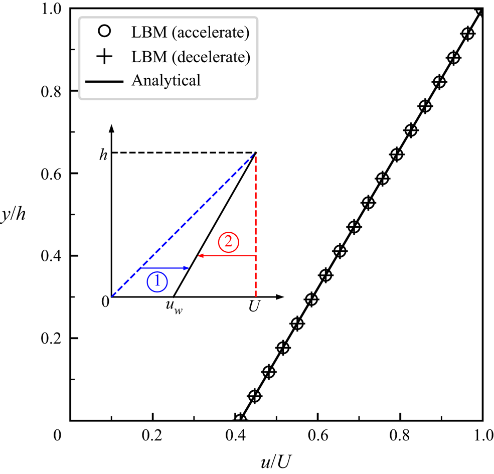
Comparison between the numerical results and the analytical solution regarding the velocity profile in plane Couette flow with  $\mu _w = 0.2$ so that a finite slip takes place at the lower wall. The inset shows two initial conditions (
 $t=0$): one with a linear velocity distribution (
 $u = yU/h$), and the other with a uniform velocity distribution (
 $u = U$) across the whole flow depth. The former is denoted by acceleration and the latter is denoted by deceleration.

3.2. Accuracy and convergence rate
In LBM simulations of the plane Couette flow, the wall separation distance  $h$ is fixed at 0.01 m, and periodic boundary conditions are defined in the
 $x$-direction. The upper wall moves with constant velocity 1.0 m s
 $^{-1}$, and different friction coefficients are adopted for the lower frictional wall, so that both no-slip and slip (i.e. partial-slip and free-slip) conditions are simulated. The fluid density
 $\rho$ and the dynamic viscosity
 $\eta$ are set to be 1500 kg m
 $^{-3}$ and 0.5 Pa s, respectively. Taking the velocity of the upper wall and the wall spacing as the characteristic velocity and length scales, we can get that the Reynolds number of the problem is 30. The gravitational acceleration
 $g$ is set to be 9.81 m s
 $^{-2}$. As for the numerical resolution, the lattice spacing and the time step are varied consistently by following the so-called diffusive scaling (Krüger, Varnik & Raabe Reference Krüger, Varnik and Raabe2010), i.e.
 $\Delta t \propto \Delta x^2$, so that the same relaxation time (
 $\tau = 0.8$) can be applied for a fixed fluid viscosity in physical units; see (2.4).
To obtain the critical friction coefficient below which wall slip will occur, the wall slip velocity  $u_w$ is set to be 0 in (3.3), and the resulting critical value is about 0.34. It is first interesting to test whether the newly proposed boundary condition is able to capture the velocity profile across the whole flow depth when there is a finite slip at the lower frictional wall. Therefore, a small friction coefficient
 $\mu _w = 0.2$, below the critical value, is adopted first. The resolution is set to be level 9, corresponding to 512 (i.e.
 $2^9$) lattice cells across the flow depth. As a result, the lattice spacing
 $\Delta x$ and the time step
 $\Delta t$ are equal to
 $1.953 \times 10^{-5}$ m and
 $1.144 \times 10^{-7}$ s, respectively. The velocity profile at the steady state is extracted and compared to the analytical solution, i.e. (3.2), in figure 4. Let us first look at the two different initial conditions, as shown in the inset of figure 4. Case 1 is initialized with a linear velocity distribution (
 $u = yU/h$) as indicated by the blue dashed line, while case 2 is initialized with a uniform velocity distribution (
 $u = U$) as indicated by the red dashed line. Therefore, initially, it has zero slip velocity at the lower wall in case 1, and the wall slip velocity is set to be the maximum in case 2. During the simulations, the two initial velocity profiles converge to the same steady state solution gradually, which has a finite wall slip velocity between 0 and
 $U$. Thus cases 1 and 2 are denoted by acceleration and deceleration, respectively. Figure 4 shows that both case 1 and case 2 yield roughly the same steady-state velocity profile, agreeing with the analytical solution very well. This means that the wall shear stress, which defines a one-to-one correspondence between the friction coefficient and the local shear rate according to (3.1), is also well described by the frictional boundary condition.
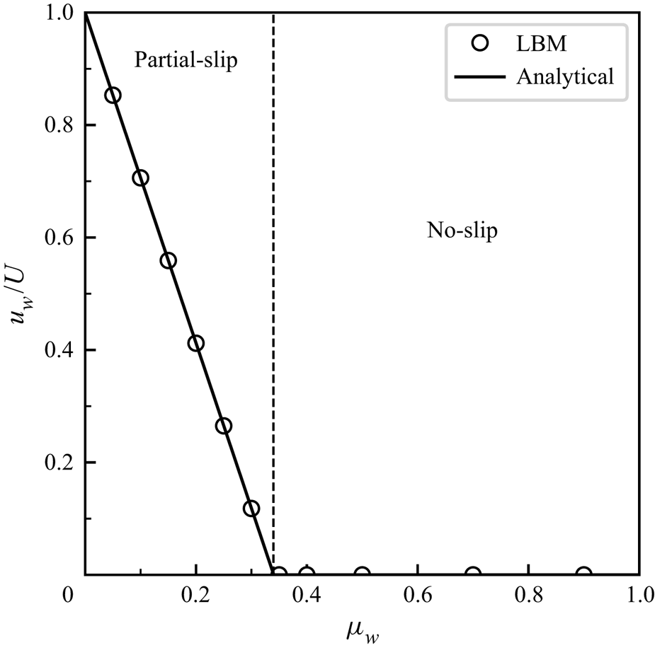
To test further the accuracy of the frictional boundary condition, different friction coefficients below and above the critical value of 0.34 are adopted. The initial condition is set to be case 1, and the resolution level is fixed at 9. Figure 5 compares the numerical results and the analytical solutions regarding the normalized wall slip velocity  $u_w/U$ at the steady state as a function of the friction coefficient
 $\mu _w$. It is found that the transition from partial-slip to no-slip at the critical friction coefficient 0.34 is captured well by the frictional boundary condition. More specifically, the wall slip velocity remains zero when
 $\mu _w$ is larger than the critical value. Meanwhile, when
 $\mu _w$ decreases from the critical value, the wall slip velocity increases, following a linear trend described by (3.3). When
 $\mu _w$ is as small as 0.05, the wall slip velocity at the lower wall is over 85 % of the maximum driving velocity at the upper wall, and further reducing the friction coefficient will approach the free-slip boundary condition.
Comparison between the numerical results and the analytical solutions regarding the normalized wall slip velocity  $u_w/U$ as a function of the friction coefficient
 $\mu _w$. The dashed line separates the partial-slip and no-slip boundary conditions.

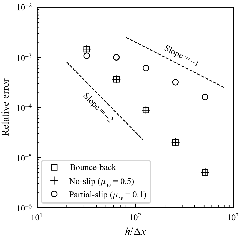
Apart from the accuracy, it is also important to check the convergence rate of the simulation when the frictional boundary condition is applied. It is well known that the Bhatnagar–Gross–Krook LBM is second-order accurate for the main body of fluid flows, and the overall convergence rate depends highly on the boundary condition (Chen et al. Reference Chen, Martínez and Mei1996; Krüger et al. Reference Krüger, Varnik and Raabe2010). We change systematically the resolution level from 5 to 9, and the resulting relative error is plotted against the lattice resolution  $h/\Delta x$ in figure 6. Here, the relative error refers to the global L2 velocity error and is calculated as
 \begin{equation} \text{relative error} = \sqrt{\frac{\displaystyle\sum (u_s - u_a)^2}{\displaystyle\sum u_a^2}}, \end{equation}
where  $u_s$ and
 $u_a$ are the numerical and analytical results for the
 $x$-component of the flow velocity, respectively. Three different boundary conditions for the lower wall are examined, referring to one bounce-back boundary condition (i.e. the conventional no-slip scenario) and two frictional boundary conditions, with one friction coefficient (0.5) above the critical value, and the other (0.1) below the critical value. Figure 6 shows that the frictional boundary condition with
 $\mu _w=0.5$ produces the same error with the bounce-back boundary condition, further confirming that the no-slip scenario associated with a rough wall can be described well by the frictional boundary condition without any deterioration of accuracy. On the other hand, in the case of partial-slip when the friction coefficient is below the critical value, the numerical error increases noticeably. The convergence rate becomes first-order, which is expected since a first-order finite difference scheme is applied to estimate the shear rate and the local pressure level at the frictional wall (see § 2.2). Further improvements can be made by using higher-order extrapolation schemes, which will increase the complexity of the boundary condition and the locality of the calculation will be lost. In addition, extra cautions have to be considered since multiple layers of fluid nodes next to the frictional wall may be unavailable due to the presence of the free surface (see figure 2).
Plot of the relative error against the lattice resolution  $h/\Delta x$ for the LBM simulation of plane Couette flow. The bounce-back boundary condition and the frictional boundary condition with different friction coefficients
 $\mu _w$ are defined for the lower wall.

All in all, the proposed frictional boundary condition is accurate and provides a unified numerical framework for the stick (no-slip) and slip behaviours at the flow–boundary interface governed by the Coulomb friction law.
4. Application to granular column collapse
4.1. Model set-up
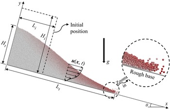
Figure 7 shows the collapse of a granular column over a rough inclined plane. The simple geometry, embedded with rich mechanical behaviours, including the complex transition between static and flow states, makes granular column collapse an ideal benchmark case for testing the performance of numerical models. Initially, the granular column is in a rectangular shape, which is depicted by the dashed lines perpendicular and parallel to the rough base in figure 7, and all particles are at rest. The initial length and height of the granular column are denoted by  $L_i$ and
 $H_i$, respectively. The granular column collapse is driven by the downward gravity, and the gravitational acceleration is
 $g=9.81$ m s
 $^{-2}$. During the collapse, the granular assembly elongates gradually along the inclined base, with the runout distance and the residual height at time
 $t$ denoted by
 $L_t$ and
 $H_t$, respectively. The symbol
 $\theta$ is used to denote the slope inclination angle. In this section, we focus on the case with
 $L_i=H_i=8$ cm and
 $\theta =0^{\circ }$.
Deposition of particles at a certain time instant after the release of a rectangular granular column on a rough inclined plane. The initial length and height of the granular column are denoted by  $L_i$ and
 $H_i$, respectively. The runout distance and the residual height are represented by
 $L_t$ and
 $H_t$, respectively. The flow front is zoomed in to show the dilute particles and the rough base.

In this study, direct numerical simulations of granular column collapses are performed using the discrete element method (DEM), which tracks the motion of individual grains according to Newton's second law, and resolves inter-particle interactions following a predefined contact model (Cundall & Strack Reference Cundall and Strack1979). Although the complex fluid–particle interactions can be considered well by coupling the DEM with a fluid solver (Jing et al. Reference Jing, Yang, Kwok and Sobral2018, Reference Jing, Yang, Kwok and Sobral2019; Yang et al. Reference Yang, Jing, Kwok and Sobral2019, Reference Yang, Jing, Kwok and Sobral2020, Reference Yang, Jing, Kwok and Sobral2021), the influence of ambient air on the collapse dynamics is considered to be negligible, which has been proved to be a valid assumption by comparing results from pure DEM simulations and experiments (Staron & Hinch Reference Staron and Hinch2005, Reference Staron and Hinch2006; Zenit Reference Zenit2005; Lacaze, Phillips & Kerswell Reference Lacaze, Phillips and Kerswell2008). While the dynamics of granular column collapse is essentially two-dimensional, our DEM simulations are actually three-dimensional so that it is more realistic. The average particle diameter is  $d_p=1$ mm with a 10 % variation around the mean. A typical value for the density of glass beads is adopted, i.e.
 $\rho _p=2500$ kg m
 $^{-3}$. The simple linear contact model is used to describe the inter-particle and particle–wall interactions. The Young's modulus
 $E$ and the normal-to-tangential stiffness ratio
 $\kappa$ are defined as
 $1.0 \times 10^9$ Pa and 1.5, respectively. Note that a reduced Young's modulus compared to glass beads is adopted so that the DEM simulation can be stable at a larger time step. Our previous study has shown that reducing Young's modulus to this extent has little effect on the collapse dynamics, but improves computational efficiency significantly (Jing et al. Reference Jing, Yang, Kwok and Sobral2019). The Young's modulus can be converted to the normal contact stiffness via
 $k_n = EA/L$, where
 $A$ and
 $L$ denote an area and a length, respectively. For particle–particle contacts,
 $A={\rm \pi} r^2$ and
 $L=r_1+r_2$, where
 $r_1$ and
 $r_2$ are the radii of the two contacting particles, and
 $r=\min (r_1, r_2)$. For particle–wall contacts, the area
 $A$ still equals
 ${\rm \pi} r^2$ but both
 $L$ and
 $r$ are defined as the radius of the particle. A damping force is applied to the contact normal direction, which can be calculated as
 $(2\beta \sqrt {m k_n})\dot {\delta }$, where
 $\beta$ is the damping ratio, and
 $\dot {\delta }$ is the relative normal velocity. The equivalent mass
 $m$ equals
 $m_1 m_2/(m_1+m_2)$ for particle–particle contacts, where
 $m_1$ and
 $m_2$ are the masses of the two contacting particles, and equals the particle mass for particle–wall contacts. A small damping ratio 0.2, which corresponds to a restitution coefficient close to 0.55, is adopted to damp the energy during inelastic collisions. The tangential force is limited by the Coulomb friction, beyond which sliding at the contact takes place, with the friction coefficient fixed at 0.5. Additional geometric roughness is introduced to the system by gluing particles of 0.5 mm diameter to the base following a simple cubic packing (Jing et al. Reference Jing, Kwok, Leung and Sobral2016); see figure 7.
Companion continuum simulations of granular column collapses are carried out using the extended LBM (LBGrain). Based on (2.13), several parameters have to be defined, apart from the local strain rate  $\dot {\gamma }$ and the pressure level
 $p$, which are accessed in real time in actual calculations. The same mean particle diameter
 $d_p$ and density
 $\rho _p$ for the DEM simulations are used in the LBGrain simulations. Note that for the bulk density of the granular flow (
 $\rho$), the voids between the solid grains have to be considered. Assuming a typical value for the packing density of densely packed granular assembly, i.e.
 $\phi =0.6$, we can get
 $\rho =\phi \rho _p=1500$ kg m
 $^{-3}$. According to Lagrée et al. (Reference Lagrée, Staron and Popinet2011), the granular column collapse undergoes higher resistances as one of the three model constants
 $\mu _s$,
 $\mu _d$ and
 $1/I_0$ increases due to the enhanced total friction, as given by (2.11). However, the collapsing dynamics is not very sensitive to those rheological parameters, and in fact fair results can be obtained through a simplified linear formulation of
 $\mu (I)$-rheology (da Cruz et al. Reference da Cruz, Emam, Prochnow, Roux and Chevoir2005); see Appendix A, especially for small inertial numbers. In this study, the model constants are selected so that the LBGrain simulations can reproduce the DEM results approximately, which are considered as the reference or the ground truth. As a result,
 $\mu _s$,
 $\mu _d$ and
 $I_0$ are set to be 0.3, 0.5 and 0.5, respectively. The regularization parameter
 $\lambda$ is set to be 0.1, which is small enough to approximate the
 $\mu (I)$-rheology (Yang et al. Reference Yang, Yang, Jing, Kwok and Sobral2023). The relaxation time
 $\tau$ is initialized to be 1.0 and will be varied according to (2.14) for this set-up. Different lattice resolutions and time steps are adopted to ensure grid independence; see Appendix B for the details. As a result, the lattice spacing
 $\Delta x$ and the time step
 $\Delta t$ are set to be
 $9.766 \times 10^{-4}$ m and
 $9.537 \times 10^{-5}$ s, respectively
Here, it is important to discuss the boundary conditions in both DEM and LBGrain simulations. In the three-dimensional DEM simulation, periodic boundary conditions are defined in the spanwise direction, and the corresponding length is 0.01 m, i.e. 10 $d_p$. Further increasing the length in the spanwise direction has little influence on the collapse dynamics. The bottom and the back of the simulation domain are enclosed by frictional walls that share the same properties of the particles. Note that the bottom wall is roughened by the glued particles (see figure 7). In this section, the simulation domain is large enough so that the entire collapse process finishes without any interference from the top and right boundaries, which are left open. However, particles will reach the right boundary and exit the simulation domain as the aspect ratio and the slope angle increase in § 5, and those particles are simply deleted. In the two-dimensional LBGrain simulation, the whole simulation domain is enclosed by frictional walls. It is worth mentioning that the macroscopic friction coefficient defined in the continuum simulation is a measure of overall energy dissipation at the boundary due to various mechanisms, including rolling, sliding and collision, which is intrinsically different from the microscopic friction coefficient at the contacts in the DEM. Generally speaking, a larger friction coefficient should be applied in LBGrain when there is a hindering effect on rolling/sliding or an enhanced collision. In this study, a small friction coefficient 0.1 is applied to the straight frictional walls in LBGrain simulations, and larger friction coefficients are adopted for the rough base. The influence of the basal friction coefficient on the collapse dynamics will be investigated in § 4.2.
4.2. Sensitivity analysis of basal friction coefficient
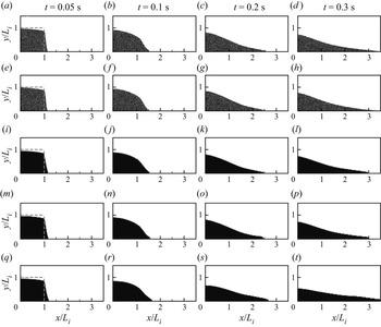
The DEM simulations of granular column collapse have been compared to and validated by experimental measurements thoroughly (Staron & Hinch Reference Staron and Hinch2005; Zenit Reference Zenit2005; Lacaze et al. Reference Lacaze, Phillips and Kerswell2008), whose results are taken as the reference or the ground truth for the calibration of basal friction coefficient in LBGrain simulations. To illustrate the important role of basal friction coefficient, series of snapshots of granular column collapses from numerical simulations using the DEM and LBGrain at  $t=0.05$, 0.1, 0.2, 0.3 s are displayed in figure 8. At first glance, the morphologies of the granular materials from LBGrain match well with those from the DEM at all time instants, showing the ability of LBGrain to model free-surface granular flows.
Snapshots of granular column collapses from numerical simulations using (a–d) DEM with a flat frictional base, (e–h) DEM with a bumpy base, (i–l) LBGrain with no-slip base, (m–p) LBGrain with frictional base ( $\mu _w=0.5$), and (q–t) LBGrain with frictional base (
 $\mu _w=0.1$) at the selected time instants (
 $t=0.05$, 0.1, 0.2, 0.3 s). The dashed lines in (a,e,i,m,q) depict the initial column geometries. Particles in the DEM simulation only with their
 $z$-coordinates in the range (
 $0.5l_z-d_p, 0.5l_z+d_p$) are shown.

Meanwhile, the basal roughness has a noticeable influence on the collapse dynamics. Comparing the DEM results from two different base conditions, one being a flat frictional wall and the other being the bumpy base defined in § 4.1, we can observe that the collapse dynamics is slightly faster and the granular deposit is more elongated when the base is flat; see figures 8(a–h). The longer runout distance is associated with a longer flow duration, indicating that the particle kinetic energy is dissipated at a lower rate. In fact, many particles at the flow front keep rolling and sliding over the flat base even after the simulation stops at  $t=0.7$ s. In this study, the resultant effect of basal roughness on the energy dissipation rate is treated as the frictional resistance at the base, which will be quantified by the basal friction coefficient in LBGrain simulations. In the following, we focus on the case with the bumpy base, whose roughness is still small so that finite slip velocities exist.
The influence of the basal friction coefficient in LBGrain simulations is also quite noticeable. When the no-slip boundary condition is applied, the runout distance  $L_t$ after 0.3 s is shorter than the DEM result with a bumpy base; see figures 8(h,l). This indicates that the continuous granular flow undergoes higher resistance than the flow of discrete particles. When the base is changed to be frictional and the basal friction coefficient is
 $\mu _w=0.5$, there is almost no change to the LBGrain simulations. That means that the basal friction coefficient is high enough to provide adequate resistance to the flow, and there exists only minor basal slip. On the other hand, when the basal friction coefficient reduces to
 $\mu _w=0.1$, the collapse dynamics becomes significantly faster. For example, at
 $t=0.3$ s, the normalized runout distance
 $L_t/L_i$ is larger than 3.5 when
 $\mu _w=0.1$, while in the other cases (including the DEM with a bumpy base) it reaches a normalized runout distance at around 3.0, see figures 8(d,h,l,p,t). Note that the basal friction coefficient has a larger influence at the later stage (i.e. after 0.2 s). This is due to the fact that the collapse dynamics is initially dominated by the fall of granular materials under gravity, and then more interactions between the flowing materials and the rough base take place afterwards.
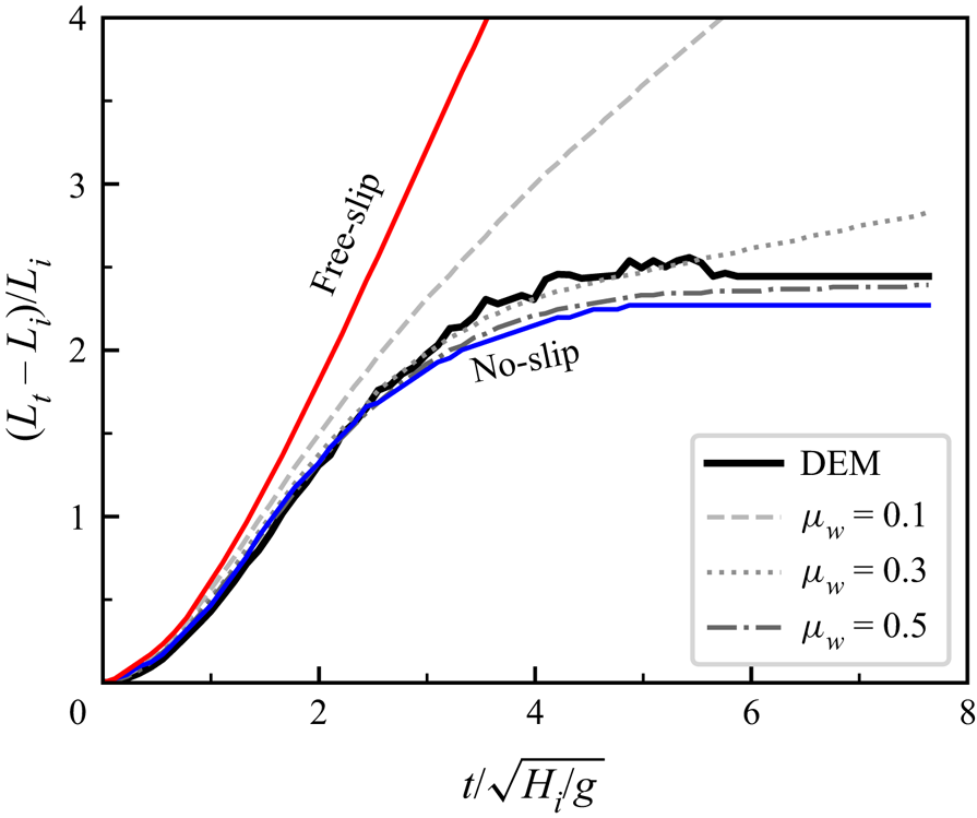
To better quantify the influence of the basal friction coefficient on the flow mobility, we plot the normalized runout distance  $(L_t-L_i)/L_i$ against the normalized time
 $t/\sqrt {H_i/g}$ in figure 9. It is relatively easier to determine the runout distance in LBGrain, which is the maximum horizontal position of a lattice cell with a non-zero fluid volume fraction. However, it becomes more difficult to extract the exact position of the flow front in the DEM, mainly due to the sparse distribution of particles at the front; see a zoom-in view in figure 7. In this study, we simply ignore the detached particles that have no contacts with the main body of the granular flow. Figure 9 shows that the LBGrain simulation cannot reproduce the DEM result if the no-slip or free-slip boundary condition is adopted. More specifically, the no-slip boundary condition underestimates the final runout distance, and the free-slip boundary condition overestimates the final runout distance drastically. The use of a frictional boundary condition results in partial-slip at the base, which is well bounded by the no-slip and free-slip boundary conditions. In addition, the collapse dynamics becomes faster and the final runout distance elongates as the basal friction coefficient decreases.
Plots of the normalized runout distance  $(L_t-L_i)/L_i$ against the normalized time
 $t/\sqrt {H_i/g}$ from the DEM simulation and the LBGrain simulations with no-slip, free-slip and frictional boundary conditions. For the LBGrain simulation with the frictional boundary condition, three basal friction coefficients are adopted, i.e.
 $\mu _w=0.1$, 0.3, 0.5.

Hence there must be a basal friction coefficient that allows LBGrain to reproduce the final runout distance in the DEM simulation. Figure 10 plots the final normalized runout distance  $(L_f-L_i)/L_i$ against the basal friction coefficient
 $\mu _w$, showing a monotonic relationship. Note that the final runout distance here refers to the value at the end of the simulation, which is 0.7 s after the release. Two different trends can be observed. When
 $\mu _w$ is less than 0.4, the final runout distance decreases quickly as
 $\mu _w$ increases, while the final runout distance reduces slightly when
 $\mu _w$ increases from 0.4 to 0.9. This saturated effect of
 $\mu _w$ at larger values or the sudden increase of mobility for
 $\mu _w$ less than a threshold is an intrinsic feature of the frictional boundary condition, which is also observed for the plane Couette flow case; see figure 5. Figure 10 shows that the LBGrain simulation with a basal friction coefficient 0.35 can capture approximately the final normalized runout distance from the DEM simulation, as indicated by the dashed line.
Plots of the final normalized runout distance  $(L_f-L_i)/L_i$ against the basal friction coefficient
 $\mu _w$. The dashed line indicates the final normalized runout distance from the DEM simulation. The solid lines show two different trends below and above
 $\mu _w=0.4$.

4.3. Internal flow characteristics
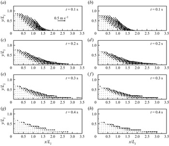
Although the runout distance is a measurable indicator for the flow mobility and sometimes has important practical implications for hazard mitigation in geophysical flows, it is measured locally and might not represent the overall flow dynamics. To examine further the performance of LBGrain and the frictional boundary condition, we fix the basal friction coefficient at 0.35 and compare the LBGrain results to the DEM regarding the internal flow characteristics. Figure 11 presents the velocity vector fields of granular column collapses at four selected time instants. When  $t=0.1$ s, the top right corner of the granular column falls down due to gravity, forming a distinguished shear plane inclined at around 45
 $^{\circ }$ to the horizontal direction, which separates the static and flow regions; see figures 11(a,b). After that, the flow direction gradually changes to be along the rough base. During flow propagation, the flowing region remains within a shallow depth below the free surface. It is due mainly to the pressure-dependent granular flow rheology; see (2.12). At shallow depth, the low pressure level results in a small apparent viscosity that promotes fluid motions. As the flow depth increases, the local pressure also increases, which is associated with the rise of apparent viscosity that inhibits fluid motions. Also, in both DEM and LBGrain simulations, there is a noticeable amount of flow velocity close to the rough base, especially at the frontal region, indicating the presence of basal slip.
Velocity vector fields of granular column collapses from numerical simulations using (a,c,e,g) the DEM and (b,d, f,h) LBGrain with a frictional base ( $\mu _w=0.35$) at the selected time instants (
 $t=0.1$, 0.2, 0.3 and 0.4 s). The length of the horizontal arrow in (a) corresponds to velocity scale 0.5 m s
 $^{-1}$.

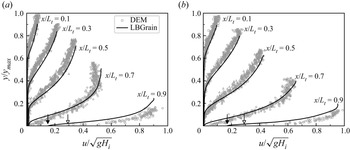
To better visualize the velocity distribution inside the flow and the slip velocity at the base, we plot in figure 12 the horizontal velocity profiles at cross-sections  $x/L_t=0.1$, 0.3, 0.5, 0.7, 0.9, and at two time instants when the flow is quite active. The vertical coordinates are normalized by the maximum flow thickness
 $y_{max}$ from the DEM simulation, and the velocities are normalized by
 $\sqrt {gH_i}$. At the back of the flow, i.e.
 $x/L_t \le 0.5$, the velocity profiles consist of a linear portion within the flowing layer beneath the granular free surface and an exponential decay inside the lower static zone. Close to the front, e.g.
 $x/L_t = 0.9$, the granular flow is active throughout the whole flow depth with a finite basal slip velocity. The filled and hollow arrows in figure 12 indicate the basal slip velocity from LBGrain and the smallest particle velocity close to the base from the DEM, respectively, at the cross-section
 $x/L_t = 0.9$. It is shown that the basal slip velocity from LBGrain is always smaller than the particle velocity close to the base from the DEM. This discrepancy will become even larger if the rough base is defined simply as no-slip in LBGrain, in which case the velocity will be zero everywhere at the base. On the other hand, the current difference is more acceptable when considering the fact that the basal slip velocity from LBGrain is accessed at the exact position of the bottom frictional wall, while the smallest particle velocity from the DEM is usually associated with the lowest particle, which is at least half a diameter above the rough base. All in all, we can conclude that LBGrain with a frictional base matches the DEM simulation regarding the velocity profiles rather well, despite the totally different natures of the two methods.
Comparison between DEM and LBGrain simulations of granular column collapses regarding the normalized velocity ( $u/\sqrt {gH_i}$) profiles at cross-sections
 $x/L_t=0.1$, 0.3, 0.5, 0.7, 0.9 when (a)
 $t=1.3\sqrt {H_i/g}$ and (b)
 $t=1.5\sqrt {H_i/g}$. The vertical positions are normalized by the maximum flow thickness
 $y_{max}$ from the DEM simulation. Different symbols represent the DEM data at various cross-sections, with only one shown in the legend.

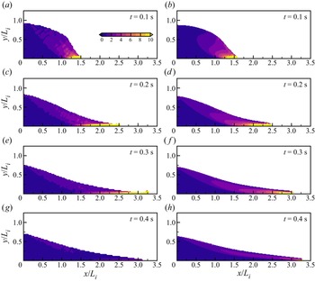
Figure 13 compares the DEM and LBGrain simulations regarding the spatial distribution of the shear rate  $\dot {\gamma }$ normalized by
 $\sqrt {g/H_i}$ at four selected time instants. The DEM results are obtained through a finite difference operation on the locally averaged velocity fields, which are less smooth compared to the LBGrain results. Nevertheless, the overall strain rate variations from the DEM and LBGrain are rather similar. More specifically, a high shear rate region can be found close to the front and near the base when the flow is active, i.e. before
 $t=0.3$ s. This high shear rate region quickly disappears from
 $t=0.3$ to 0.4 s. A closer examination of the strain rate fields at
 $t=0.2$ and 0.3 s shows that the high shear rate region from the DEM extends further back towards the static zone compared to the LBGrain results. This could be more evidence for the inadequacy of the frictional boundary condition for granular flows (Artoni & Santomaso Reference Artoni and Santomaso2014), which deserves further investigation.
Spatial distribution of the shear rate  $\dot {\gamma }$ normalized by
 $\sqrt {g/H_i}$ from numerical simulations using (a,c,e,g) the DEM and (b,d, f,h) LBGrain with a frictional base (
 $\mu _w=0.35$) at the selected time instants (
 $t=0.1$, 0.2, 0.3 and 0.4 s). All the plots share the colour bar in (a).

5. Effects of initial aspect ratio and slope angle
In § 4, we calibrate the parameters of the LBGrain model so that it agrees with the DEM simulation. However, the calibration is carried out for only one simple case, in which a square granular column collapses over a horizontal bottom plane. Meanwhile, it is well known that the dynamics of granular column collapses depends highly on the initial aspect ratio ( $H_i/L_i$), and granular material flowing on a slope is encountered commonly in nature. Therefore, it is important to test the performance of LBGrain when the slope angle and the initial aspect ratio change. In this section, we simulate two additional cases: one with the geometry of the granular column unchanged and the slope angle increased from 0 to 15
 $^{\circ }$; the other with the initial column length
 $L_i$ and height
 $H_i$ adjusted to 5 and 10 cm, respectively, so it gives initial aspect ratio 2. In the DEM simulations, the material properties and the rough base remain unchanged. Ideally, the LBGrain results should match the DEM results automatically by simply changing the column geometry or the gravity orientation correspondingly, without any further adjustments to the rheological parameters and the basal friction coefficient.
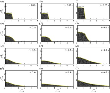
Snapshots of granular column collapses at  $t=0.05$, 0.1, 0.2 and 0.3 s from the DEM simulations. Only particles with
 $z$-coordinates in the range
 $(0.5l_z-d_p, 0.5l_z+d_p)$ are shown. The initial aspect ratio and the slope angle are (a–d) 1 and 0, (e–h) 1 and 15
 $^{\circ }$, and (i–l) 2 and 0, respectively. The dashed lines in (a,e,i) depict the initial column geometries. The yellow solid lines are the free-surface profiles extracted from the companion LBGrain simulations at the corresponding time instants.

5.1. Macroscopic observations
Figure 14 presents snapshots of granular column collapses at  $t=0.05$, 0.1, 0.2 and 0.3 s from the DEM simulations. The yellow solid lines are the free-surface profiles extracted from the companion LBGrain simulations at the corresponding time instants. For the original case with the initial aspect ratio
 $a$ and the slope angle
 $\theta$ equal to 1 and 0, respectively, as shown in figures 14(a–d), the granular column collapse initiates with the fall of the top right corner. The residual height drops only slightly within the first 0.1 s. After that, the runout distance elongates further, and at
 $t=0.3$ s, the free-surface profile has a concave shape. When the slope angle
 $\theta$ increases to 15
 $^{\circ }$, as shown in figures 14(e–h), the collapse dynamics becomes totally different. At
 $t=0.1$ s, the residual height drops significantly, and the upper surface of the granular column becomes more rounded and is in a convex shape. The granular deposits at
 $t=0.2$ and 0.3 s are thinner and longer compared to the original case, indicating a higher flow mobility. At
 $t=0.3$ s, the free-surface profile is quite linear, and the column height is more than halved. When the initial aspect ratio
 $a$ increases to 2, as shown in figures 14(i–l), the vertical fall of the granular column becomes more prominent, similar to the collapse on the slope. At
 $t=0.3$ s, the maximum flow thickness is about halved and the runout distance normalized by
 $L_i$ is the longest, which exceeds 5. The free-surface profile, on the other hand, has a slightly concave shape, similar to the original case. In all three cases tested in this study, with different slope angles and initial aspect ratios, the LBGrain model is able to capture the free-surface evolution from the DEM simulations very well using the same set of model parameters.
Plots of the normalized runout distance  $(L_t-L_i)/L_i$ against the normalized time
 $t/\sqrt {H_i/g}$ from the DEM and LBGrain simulations with various initial aspect ratios and slope inclination angles.

Figure 15 compares the temporal evolution of the normalized runout distance  $(L_t-L_i)/L_i$ from the DEM and LBGrain simulations. Again, the runout behaviours are totally different when the slope angle or the initial aspect ratio changes. In terms of the normalized quantities, the rate of acceleration is the largest when the initial aspect ratio increases to 2, but the final runout distance is the longest when the slope angle increases to 15
 $^{\circ }$. In fact, the final runout distance in the case with
 $\theta =15^{\circ }$ would be even longer, which is here limited by the size of the simulation domain, i.e.
 $l_x=0.5$ m. This is the reason why the runout distance suddenly stops increasing at around
 $t=6\sqrt {H_i/g}$ in both the DEM and LBGrain simulations; see the red lines in figure 15, and supplementary movie 1 (available at https://doi.org/10.1017/jfm.2023.782). On the other hand, the simulation domain is large enough to enclose the final deposit of the case with
 $a=2$. Interestingly, although the final normalized runout distance is about doubled when
 $a$ increases from 1 to 2, the flow deposition finishes at approximately the same normalized time, i.e.
 $t=4\sqrt {H_i/g}$. It agrees with our previous finding that the term
 $\sqrt {H_i/g}$ is the relevant time scale for the measure of flow duration in granular column collapse problems (Jing et al. Reference Jing, Yang, Kwok and Sobral2018). All in all, the LBGrain model agrees with the DEM simulation regarding the runout evolution throughout the whole flow duration for different slope angles and initial aspect ratios.
5.2. Flow kinematics
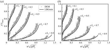
Apart from the morphologies of the granular deposits during the collapses, it is also vital to capture the flow kinematics in the two generalized cases. Figure 16 compares the DEM and LBGrain simulations regarding the velocity profiles at five selected cross-sections when  $t=1.5\sqrt {H_i/g}$. Similarly to figure 12, the vertical position and the horizontal velocity are normalized by the maximum flow thickness
 $y_{max}$ in the DEM and
 $\sqrt {gH_i}$, respectively. First, the velocity profiles from LBGrain (solid lines in figure 16) almost overlap with the particle velocities from the DEM (markers in figure 16), demonstrating the predictability of the continuous LBGrain model.
Comparison between DEM and LBGrain simulations of granular column collapses regarding the normalized velocity ( $u/\sqrt {gH_i}$) profiles at cross-sections
 $x/L_t=0.1$, 0.3, 0.5, 0.7, 0.9 when
 $t=1.5\sqrt {H_i/g}$. The initial aspect ratio and the slope angle are (a) 1 and 15
 $^{\circ }$, and (b) 2 and 0, respectively. The vertical positions are normalized by the maximum flow thickness
 $y_{max}$ from the DEM simulation. Different symbols represent the DEM data at various cross-sections, with only one shown in the legend.

When the slope angle is 15 $^{\circ }$ and the initial aspect ratio is 1, as shown in figure 16(a), a small finite basal slip velocity is observed at
 $x/L_t=0.7$, which is absent when the slope angle is 0; see figure 12(b). In addition, at the cross-section
 $x/L_t=0.9$, the basal slip velocity in LBGrain and the smallest particle velocity in the DEM increase significantly as the slope angle increases. When the slope angle is 0 and the initial aspect ratio is 2, as shown in figure 16(b), a noticeable basal slip is still present at the cross-section
 $x/L_t=0.7$. And the basal slip velocity in LBGrain and the smallest particle velocity in the DEM at the cross-section
 $x/L_t=0.9$ also become larger compared to the case with initial aspect ratio 1. This further highlights the importance of applying a partial-slip boundary condition, e.g. the frictional boundary condition in this study, for the simulation of dense granular flows, especially when the flow mobility is high, which can be caused by the flow over an inclined slope or a high initial potential energy.
The kinetic energy of the granular flow is also monitored in both DEM and LBGrain simulations during the whole flow process. From the physics perspective, we use the evolution of kinetic energy as an indicator for flow regime transitions caused by the initial aspect ratio and the packing density when the pore fluid effects cannot be ignored, as in our previous studies (Jing et al. Reference Jing, Yang, Kwok and Sobral2018; Yang et al. Reference Yang, Jing, Kwok and Sobral2020). In engineering practice (e.g. the risk assessment of landslides), the kinetic energy of the granular flow usually provides an upper bound for the impact energy on the resisting structures along the flow path (Utili, Zhao & Houlsby Reference Utili, Zhao and Houlsby2015). Figure 17 compares the temporal evolution of the kinetic energy  $E_k$ from the DEM and LBGrain simulations of granular column collapses with various initial aspect ratios and slope inclination angles. Note that the rotational component of the kinetic energy in the DEM, which is not available in LBGrain, is found to be negligible, and only the translational kinetic energy is considered. Another difference is the dimension (the DEM is three-dimensional, and LBGrain is two-dimensional), which has been taken into account by normalizing the kinetic energy
 $E_k$ by the initial potential energy
 $E_0$ of each case.
Comparison between DEM and LBGrain simulations of granular column collapses, with different initial aspect ratios and slope inclination angles, regarding the temporal evolution of the translational kinetic energy  $E_k$, which is normalized by the initial potential energy
 $E_0$ of each case.

Figure 17 shows that the two granular column collapses over the horizontal bottom plane ( $\theta =0$) reach the peak kinetic energy at around
 $t=1.5\sqrt {H_i/g}$. The maximum
 $E_k/E_0$ value becomes significantly larger as the initial aspect ratio
 $a$ increases, indicating that a higher percentage of the potential energy is transferred to the kinetic energy during the collapse of tall granular columns, resulting in a higher flow mobility and a longer runout distance. For the case with
 $a=1$ and
 $\theta =15^{\circ }$, the peak kinetic energy is reached at a later stage (around
 $t=2.5\sqrt {H_i/g}$), and the maximum
 $E_k/E_0$ value becomes even larger with the kinetic energy covering over 25 % of the initial potential energy. Taking the DEM results as the reference, the LBGrain model overestimates the peak kinetic energy by at least 11.6 %, which will lead to more conservative designs of countermeasures when considering the kinetic energy as a measure of the destructive power of granular flows. Apart from that, the effects of the initial aspect ratio and the slope angle on the kinetic energy are well described by LBGrain, producing the same trend with the DEM simulations.
5.3. Discussion and limitations
Among numerous researches on the simulation of granular flows, the DEM is still considered one of the most sophisticated methods because of its discrete nature and the relatively few assumptions. All the numerical data are accessible either directly or indirectly via local average, such as the spatio-temporal distribution of flow velocity and energy inside the flow, which are usually very difficult to be measured in laboratory experiments. However, the use of the DEM for large-scale granular flow simulations is also limited due to its high computational cost. For example, the DEM modelling of granular column collapses in this study, consisting of more than 70 000 particles, take several days to finish just 0.7 s of simulation in physical time. By contrast, the companion LBGrain simulations take only a few minutes.
Although no special treatment of the boundary condition is required in the DEM, aside from the normal particle–wall and particle–particle interactions, the definition of proper boundary conditions in continuum models becomes exceptionally tricky, being neither no-slip nor free-slip. In this study, we propose a frictional boundary condition in the lattice Boltzmann framework as a first-order approximation to the stick–slip behaviour of granular flows at the boundary. We find that after the calibration against one simple DEM simulation, i.e. a square granular column collapsing over a horizontal bottom plane, the LBGrain model is capable of simulating granular column collapses in other scenarios with different initial aspect ratios and slope inclination angles. It highlights the generalization ability of LBGrain, due mainly to the physics-informed rheology and boundary condition, which is essential for any practical prediction of the complex granular flow behaviours.
Nevertheless, the limitations of the frictional boundary condition described by a constant friction coefficient should not be overlooked. For instance, the frictional boundary condition will predict a sharp transition between no-slip and constant acceleration in an inclined chute flow, in which a steady slip state is possible only when  $\tan \theta =\mu _w$. However, the actual behaviour of the granular chute flow is that a steady state with a finite basal slip velocity can be obtained with a wide range of
 $\tan \theta <\mu _w$ (Artoni & Santomaso Reference Artoni and Santomaso2014). The close agreement between the DEM and LBGrain in this study could be due to the fact that the overall dynamics of transient granular column collapses is dominated by the average basal resistance, which can be described well by a single friction coefficient after calibration. And there seems to be a one-to-one relationship between the friction coefficient and the geometric roughness of the boundary, which deserves further investigations in more detail in a future study. Recently, detailed measurements of stresses and flow kinematics at the boundary, both numerically and experimentally, provide opportunities for discovering emerging boundary conditions for dense granular flows, e.g. the weakening of effective wall friction and its scaling with the interface properties in various flow configurations (Artoni & Richard Reference Artoni and Richard2015; Yang & Huang Reference Yang and Huang2016; Artoni et al. Reference Artoni, Soligo, Paul and Richard2018; Roche et al. Reference Roche, van den Wildenberg, Valance, Delannay, Mangeney, Corna and Latchimy2021). The numerical framework proposed in this study can be extended easily to model a dynamic friction coefficient, as long as the relevant flow quantities for scaling are accessible during simulations.
6. Conclusions
In this paper, we propose a novel frictional boundary condition within the lattice Boltzmann framework for better numerical simulations of dense granular flows. We adopt a hybrid approach that first calculates the wall slip velocity based on the shear rate limited by the Coulomb friction, followed by the reconstruction of unknown density distribution functions through the modified bounce-back scheme. The newly proposed boundary condition has several advantages, including the easy implementation in existing LBM codes and the conservation of mass up to machine precision with the presence of a free surface.
To validate the numerical model, we simulate a modified plane Couette flow bounded by two infinite parallel walls. The upper wall is no-slip and has a constant velocity driving the fluid flow. The lower wall is stationary but becomes frictional so that wall slip occurs when the shear stress exceeds a critical threshold defined by the Coulomb friction. Analytical solutions for the velocity profile and the wall slip velocity, as functions of the friction coefficient, are derived. We carry out LBM simulations with various friction coefficients and find excellent agreement with the analytical solutions, including the regime transition between no-slip and partial-slip. A close examination of the convergence rate shows that the frictional boundary condition is second-order accurate when there is no slip, but it drops to first order when slip occurs. Further improvements should be made to increase the order of accuracy, so that the same convergence rate (i.e. second order) with the main body of the fluid flow calculation can be achieved.
After validation, the LBM model is applied to simulate granular column collapse, which has been well recognized as a model case to study geophysical flows. Discrete element simulations are also carried out, whose results are considered to be accurate and are taken as the reference to examine the performance of the LBM model. The rheological parameters and the friction coefficient in LBM are first calibrated for a simple case of a square granular column collapsing over a horizontal bottom plane, i.e.  $a=1$ and
 $\theta =0$. The calibrated LBM model agrees with the companion DEM simulation in terms of both the macroscopic observations of granular deposit morphologies and the complex internal flow structures, i.e. the spatio-temporal distributions of flow velocity and shear rate. The use of a commonly adopted no-slip boundary condition for the rough base underestimates the runout distance and cannot reproduce the non-zero basal slip velocity, which is present in the DEM simulation, especially close to the flow front.
Then the calibrated LBM model for granular column collapse is applied to study the effects of initial aspect ratio  $a$ and the slope angle
 $\theta$. It is found that the LBM model automatically matches the DEM simulation for cases with different
 $a$ and
 $\theta$ values, without any further adjustments to the model parameters. The successful simulation of the generalized cases demonstrates the predictability of the LBM model and the proposed frictional boundary condition for dense granular flows. Benefitting from easy access to all the numerical data, such as the flow kinetic energy, the proposed method has the potential to become an alternative numerical tool for large-scale geophysical flow predictions, and aid the design of mitigation measures. Our future work will focus on the extension of the frictional boundary condition for curved walls, and the improvement of the computational efficiency through heterogeneous computing.
Comparison of free-surface profiles of granular column collapses at  $t=0.05$, 0.1, 0.2 and 0.3 s from the LBGrain simulations with the linear and nonlinear formulations of
 $\mu (I)$-rheology. The initial aspect ratio and the slope angle are (a–d) 1 and 0, (e–h) 1 and 15
 $^{\circ }$, and (i–l) 2 and 0, respectively. The grey dashed lines in (a,e,i) depict the initial column geometries.

(a) Plot of the normalized runout distance  $(L_t-L_i)/L_i$ against the normalized time
 $t/\sqrt {H_i/g}$ at different resolution levels. (b) Comparison of the free-surface profiles at different resolution levels when
 $t=0.1$, 0.2 and 0.4 s. The grey dashed line depicts the initial column geometry. Note that the horizontal and vertical axes are not to scale.

Supplementary movie
A supplementary movie is available at https://doi.org/10.1017/jfm.2023.782.
Funding
This research was developed under the support of the NSFC project no. 42107154 and the Guangdong basic and applied basic research foundation nos 2020A1515110810 and 2023A1515012881, the Hong Kong GRF projects nos 17205821 and 17205222 and the FAP-DF project no. 00193-00001155/2021-40, Brazil.
Declaration of interests
The authors report no conflict of interest.
Appendix A. LBGrain results with the linear formulation of  $\mu (I)$-rheology

The  $\mu (I)$-rheology defined by (2.11) relates the friction coefficient to the inertial number nonlinearly with a smooth transition from the minimum (
 $\mu _s$) to the maximum (
 $\mu _d$) values. Sections 4 and 5 demonstrate that this nonlinear formulation of
 $\mu (I)$-rheology is capable of capturing the collapsing dynamics of granular columns with various aspect ratios and on different slopes. Meanwhile, one may question the necessity of using a nonlinear model since the influence of the model parameters on the collapsing dynamics is relatively small (Lagrée et al. Reference Lagrée, Staron and Popinet2011). Therefore, we performed an additional set of LBGrain simulations using the linear formulation of
 $\mu (I)$-rheology (da Cruz et al. Reference da Cruz, Emam, Prochnow, Roux and Chevoir2005),
 $\mu (I) = \mu _s + bI$, which has two model parameters, namely
 $\mu _s$ and
 $b$. We calibrated the linear model regarding the temporal evolution of runout distance when the initial aspect ratio and the slope angle are 1 and 0, respectively. The resulting model parameters are
 $\mu _s = 0.22$ and
 $b = 0.7$.
Figures 18(a–d) compare the free-surface profiles of granular column collapses from the linear and nonlinear models at  $t=0.05$, 0.1, 0.2 and 0.3 s. The linear and nonlinear models produce rather similar results. When the slope angle increases to
 $15^{\circ }$, the free-surface profiles from the linear and nonlinear models are still visually similar to each other before
 $t=0.1$ s; see figures 18(e, f). However, the granular deposit from the nonlinear model becomes slightly more elongated after
 $t=0.2$ s, as shown in figures 18(g,h). A similar behaviour can be observed when the initial aspect ratio increases to 2; see figures 18(i–l). The good agreement between the linear and nonlinear models during the early stage indicates that the two models perform similarly for small inertial numbers. However, the linear model predicts the increase of
 $\mu$ with
 $I$ without any saturation. It is likely the reason why the linear model results in a shorter final runout distance when larger inertial numbers are encountered during the later stage of collapse for steeper slopes and taller columns, due to the larger total friction.
Appendix B. Convergence analysis of granular column collapse
It is important to ensure that an adequately high lattice resolution is adopted to achieve grid independence of LBGrain simulations. We simulate the granular column collapse on a horizontal bottom plane with the initial height  $H_i$ and length
 $L_i$ both equal to 8 cm, i.e. the case we used for calibration in § 4. The dimensions of the simulation domain in the
 $x$- and
 $y$-directions are 0.5 and 0.2 m, respectively. LBGrain simulations with three different levels of lattice resolution, referring to 8, 9 and 10 for 256, 512 and 1024 lattice cells along the
 $x$-direction, are tested. When the lattice spacing
 $\Delta x$ varies, the ratio
 $\Delta x^2 / \Delta t$ is kept constant at 0.01 so that the Mach number is small and the compressibility error is maintained at a low level for all resolutions.
Figure 19(a) presents the temporal evolution of the normalized runout distance  $(L_t-L_i)/L_i$. Before
 $t=0.5\sqrt {H_i/g}$, there is a negligible influence of the lattice resolution on the runout distance. However, the granular column collapses at a faster rate as the resolution level increases at the later stage. During deposition, the deposit elongates slowly at level 8 without a clear sign of stoppage, similar to creeping. It is potentially caused by the large influence of regularization at a coarser resolution. The deposits almost stop deforming after
 $t=5\sqrt {H_i/g}$ at levels 9 and 10, with the latter propagating slightly farther.
Figure 19(b) compares the free-surface profiles at three different resolution levels when  $t = 0.1$, 0.2 and 0.4 s. It is shown that the free-surface profiles at different resolution levels and time instants are rather similar, indicating that the overall collapse dynamics is affected only slightly for the three tested resolutions. A larger difference is observed close to the horizontal and vertical walls, which could be due to the lower convergence rate of the frictional boundary condition when slip occurs. In this study, to balance the computational accuracy and efficiency, the resolution level 9 is adopted for the LBGrain simulation of granular column collapses.