On the eve of the election, the impending result of the presidential vote can be seen fairly clearly from trial-heat polls. Earlier in the election year, the polls offer much less information about what will happen on Election Day (see Campbell Reference Campbell2008; Wlezien and Erikson Reference Wlezien and Erikson2002). The polls capture preferences to the moment and do not—because they cannot—anticipate how preferences will evolve in the future, as the campaign unfolds. Various things ultimately impact the final vote. The standing of the sitting president is important. The economy is too. Both can change as the election cycle evolves. To make matters worse, late-arriving economic shocks have a bigger impact on the electoral verdict than those that arrive earlier. This complicates accurately forecasting the vote well in advance.
Our solution to the problem of early forecasting has been to turn to the index of leading economic indicators (LEI). In previous papers (Wlezien and Erikson Reference Wlezien and Erikson1996; Reference Wlezien and Erikson2001; Reference Wlezien and Erikson2004; Reference Wlezien and Erikson2005; Erikson and Wlezien Reference Erikson and Wlezien2008) we have shown that the growth in these indicators through the spring of the election year—quarter 13 of the election cycle—is a strong predictor of the vote. This is for two reasons: (1) it gives advance indication of changes in the economy (and presidential approval) during the election year; and (2) it provides a comprehensive summary of the state of the economy leading up to the election year. Here we update our analysis to incorporate the most recent 2004 data point, bringing the number of cases in our model to a grand total of 14, the set of elections between 1952 and 2004. We focus specifically on how the early quarter 13 measure of LEI growth works to predict the vote in conjunction with trial-heat polls at different points during the election year. Based on the results, we offer forecasts for 2008 using information available at the time of this writing (August 1, 2008). Given the weak growth in leading economic indicators, the forecasts point to a cautious prediction of a Barack Obama victory.
Leading Economic Indicators and the Vote
The crucial variable in our forecasting exercise is the cumulative quarterly growth in leading economic indicators over the course of the sitting president's term.Footnote 1 The measure is the weighted average of quarterly summaries of monthly growth, with each quarter weighted 0.90 times as much as the following quarter (1.11 times the weight of the preceding quarter). This weighting scheme maximizes the correlation with the presidential vote, which peaks using quarter 13 indicators, through the first quarter—the end of March—of the election year. For additional, important detail about the construction of the measure, see the Appendix.
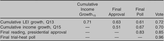
Our measure of LEI growth is a good predictor of Election Day conditions. The relationships are clear in Table 1, which shows bivariate correlations between cumulative LEI growth and final pre-election measures of two well-known predictors of the vote—per capita income growth and presidential approval—as well as the final pre-election poll and the actual vote itself. The data relate to the 14 elections between 1952 and 2004. We measure income growth cumulatively over the presidential term, through the 15th quarter of the cycle, ending in September, weighting each quarter's reading 0.80 times the one that follows.Footnote 2 Presidential approval is the percent approving of the job the president is doing in the final pre-election Gallup Poll. The trial-heat poll and vote variables measure the incumbent-party share of the two-party vote, ignoring third-party candidates.Footnote 3
Correlations, 1952–2004
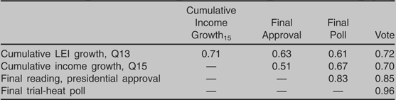
In Table 1 we see that the quarter 13 measure of cumulative LEI growth nicely predicts the final, quarter 15 measure of cumulative income growth. The correlation is 0.71. Notice as well in Table 1 that leading indicators predict the final, pre-election reading of presidential approval from the Gallup Poll. The correlation (0.63) is modest by comparison with what we saw for income growth, which is as we would expect. That is, evaluations of sitting presidents reflect economics and other things. Most importantly, LEI growth correlates well with the incumbent-party share of the final pre-election poll and, even more so, the presidential vote. Approval still is a better predictor but the polls are best of all. Indeed, the correlation between the final pre-election poll results and the vote is a near-perfect 0.96. They tell us almost everything about what will happen on Election Day.
Forecasting the Presidential Vote
Now, let us see what we can foresee at different points in the election cycle, following our previous research (especially Wlezien and Erikson Reference Wlezien and Erikson2004). Our dependent variable is the incumbent-party share of the two-party vote. We use but two independent variables: (1) the quarter 13 measure of cumulative LEI growth; and (2) current quarterly trial-heat election poll results, measured as the incumbent-party share of the two-party vote. The trial-heat variable is the average share in polls during each particular quarter.Footnote 4
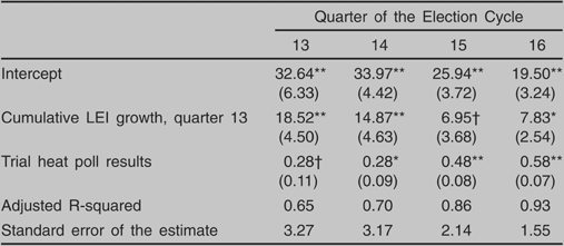
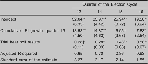
Table 2 shows the results of regression analysis for the final four quarters of the election cycle. These results are as expected. The predictive power of LEI is greatest (and most reliable) in the “quarter 13” model, using trial-heat polls from the first quarter of the election year. It drops off some in later quarters as more updated information from the polls is used, which increasingly reflects the changes in the economy (and presidential approval) predicted by early leading indicators. The contribution of the polls increases correspondingly. By the end of the cycle, our measure of cumulative LEI growth and the polls are highly correlated with each other, as we saw in Table 1. The growth in leading economic indicators through quarter 13 still predicts the vote independently of the polls even in the final model, using polls from October and November. This indicates that some effects of the economy register with voters during the last few weeks of the campaign.
Predicting the Presidential Vote, 1952–2004
Note: N = 14. Numbers in parentheses are standard errors. Cumulative LEI Growth = summed weighted growth in leading economic indicators through quarter 13 of the election cycle, with each quarter weighted 0.9 times the following quarter. Trial-heat poll results are for the quarter (13 through 16) indicated.
† p < .10;
* p < .05;
** p < .01 (two-tailed).
This analysis affords us a preliminary forecast of the 2008 vote. We merely need to input the 2008 value of LEI growth and appropriate quarterly poll figures. Through the first quarter of 2008 (quarter 13 of the election cycle), the value of LEI growth is −0.049. The number is well below average over the last 15 presidential election years (mean = 0.16, s.d. = 0.35). It actually is one of only two times when the cumulative growth has been negative, the other being in 1980, when LEI growth was an abysmal −0.294. The low number for 2008 does not surprise much now, in the summer of 2008. It may have been more surprising in the early-spring, however. Economic problems could already be seen at the end of 2007, as LEI growth through quarter 12 foreshadowed a weak election-year economy.Footnote 5 This bodes poorly for John McCain's presidential aspirations.
For the polls we turn to RealClearPolitics.com, which reports 50 polls pitting Obama and McCain during the second quarter of the year, April–June. The average share in these polls is 46.6% for McCain, which also bodes poorly for the Arizona senator. Plugging the LEI and poll numbers into the quarter 14 equation in Table 2 predicts a vote share of 46.2% for McCain, 53.8% for Obama. An Obama advantage could be seen even earlier on, using polls from the first quarter of the election year. Plugging in the average share in the 39 Obama-McCain polls conducted between January and March together with LEI growth through the same quarter, the quarter 13 equation in Table 2 predicts a slightly larger share for Obama, 54.8%.Footnote 6
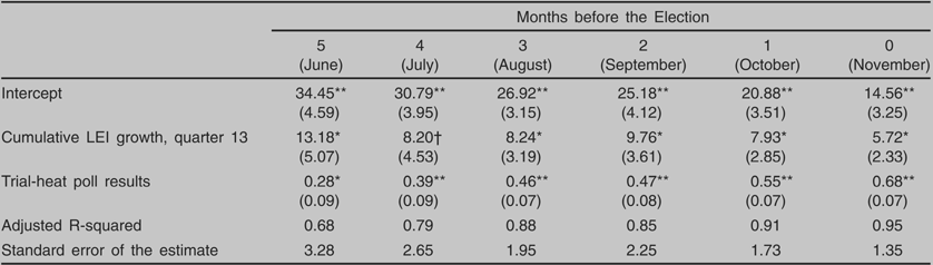
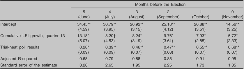
The quarterly analysis provides a very coarse picture. We can provide a more fine-grained analysis using monthly polls. Table 3 shows the regressions predicting the incumbent-party vote from quarter 13 cumulative LEI growth and the incumbent candidate's share in the polls taken in each month prior to Election Day and also at the very end of the cycle. In the table we can see that the quarterly analysis conceals important dynamics, particularly during the depths of summer. As can be seen from the explained variances, polls improve our ability to predict the vote quite a lot as we move into July and August. Over the ensuing months, the polls increasingly incorporate the economic change predicted by early LEI growth and also other important information about the candidates. The size and significance of the polls' effect on the vote thus increase markedly and the effect of LEI growth declines. Yet again, the quarter 13 measure of LEI growth predicts the vote independently of the polls even in the final model, here using final pre-election polls. The result suggests that the electorate does not fully factor in important election-year economic changes until Election Day itself (also see Brown and Chappell Reference Brown and Chappell1999; Campbell Reference Campbell2008; Wlezien and Erikson Reference Wlezien and Erikson2004).
Forecasting during the Last Five Months, 1952–2004
Note: N = 14. Numbers in parentheses are standard errors. Cumulative LEI Growth = summed weighted growth in leading economic indicators through quarter 13 of the election cycle, with each quarter weighted 0.9 times the following quarter. Trial-heat poll results are for the month indicated.
† p < .10;
* p < .05;
** p < .01 (two-tailed).
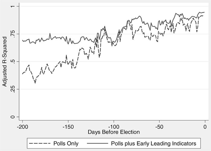
Figure 1 shows how much LEI growth contributes to our ability to predict the vote beyond what is available in the polls over the course of the election year. The figure displays two series of numbers. The first series is the R-squareds (across the 14 election years) from regressing the vote division on the poll division for each date starting 200 days before the election. This is the first day for which we have poll results in each of the 14 election years. The second series is the R-squareds from regressing the vote division on the poll division for each date and quarter 13 LEI growth. In other words, for the second series we exactly follow what we did in Tables 2 and 3 but use polling numbers for each day instead of each quarter or month.Footnote 7
Forecasting using Polls and Early Leading Economic Indicators as the Election Campaign Unfolds, 1952–2004
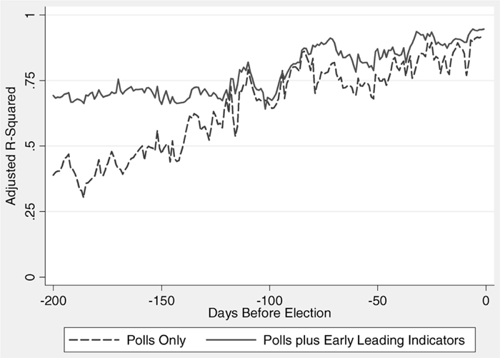
In the figure we can see that the performance of the polls over the period varies a lot. Early on, 200 days before Election Day, the polls explain about 40% of the variance in the vote. The number increases using later polls in an almost linear fashion until the very end of the campaign. The performance of the model including LEI growth indicates that much of this gain in predictability reflects the fact that the polls increasingly absorb the economic change foreshadowed by early leading economic indicators. That is, the model performs equally well using poll data from about 125–200 days before Election Day, when the R-squareds hover between 70 and 75%. We see a steady improvement in predictability thereafter, during the last 125 days of the campaign. Even as the polls do not ever completely incorporate economic effects on the final vote, they do pick up other aspects of preferences, some of which are not known or even knowable in advance. This improves our forecasts leading up to Election Day.
Forecasting 2008
The foregoing analysis reveals the important impact of temporal horizons on election forecasting. Forecasts made at different points in time can differ meaningfully depending on the available information. At the time of this writing, August 1, more than three months before Election Day, our best forecast is based on LEI growth through quarter 13 plus trial-heat polls for the most recent month, July. We plug the 2008 values of cumulative LEI growth and the available July polls into the “July” equation from Table 3.
Recall that the value of LEI growth in 2008 is −0.049. As we have noted, this variable rarely has taken on negative values in the past. As for the polls, RealClearPolitics.com shows results for 14 surveys pitting Obama against McCain during July. In these polls, McCain's two-party share is 47.8%. Plugging this number and the LEI estimate into the July equation in Table 3 predicts 49.2% of the two-party vote for McCain, 50.8% for Obama.
This forecast based on July polls lowers the expectation of the Obama vote from the preliminary forecast based on LEI growth plus earlier quarter 14 polls, discussed above. Obama's poll numbers did not surge in July the way that early leading economic indicators predict—indeed, his July poll share was largely unchanged from the previous quarter. Even still, the advantage from the July forecast is with Obama. This advantage is best expressed as the probability of winning the majority of the vote. We compute the p-value using the forecast itself, the standard forecast error, and the t distribution (with 11 degrees of freedom).Footnote 8 Based on the statistical history of the model, we estimate Obama's chances at the moment to be 0.60, or about three chances in five.
The July forecast for 2008 may be somewhat deceiving in that in July 2008 the conventions were still a long way off, whereas in earlier years the convention season almost always had began and sometimes even finished during July. This poses two challenges for our analysis. First, in previous election years, with the conventions as a focus, the public might have more clearly factored in the economy by July. Second, since only the out-party convention usually will have taken place, the post-convention bounce in the polls that the out-party receives will tend to force an in-party bonus into the equation.Footnote 9 In late-July, 2008, we were still four weeks away from the Democratic Party Convention. To see what difference this may make, we revise our forecasting equation to take into account the convention timing. To do this, we reestimate the equation across the previous 14 elections using polls from 28 days before the first convention.Footnote 10 That resulting equation is:

In the equation we can see that the coefficient for LEI growth is larger and the coefficient for the polls correspondingly lower by comparison with the July equation in Table 3. This is exactly as we expected. Plugging in the same values of LEI growth and the July McCain poll share now predicts 47.0% for McCain, 53.0% for Obama. This is very close to our predictions using polls from the first half of the election year, and implies that little has changed since then. Applying the forecast error and the t-distribution, the probability that Obama will win the popular vote is 0.78, or about four chances in five.
An Updated (Pre-Convention) Forecast
Our final forecast at deadline is based on McCain's showing in August trial-heat polls posted prior to the Democratic convention on RealClearPolitics.com (48.0%). The forecast equation is estimated across the previous 14 elections using polls from seven days prior to the first convention:Footnote 12
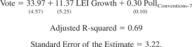
Plugging in the poll share (48.0) for McCain, the incumbent party candidate, and the 2008 value of LEI growth (−0.049) yields 47.8% for McCain, 52.2% for Obama as the expectation in the run-up to the conventions. Taking into account the forecast error, the win-probabilities are 0.28 for McCain and 0.72 for Obama. Obama's modest win-advantage in our model thus held (fairly) steady through August 2008 even as his forecast share of the vote has declined. His poll margins just did not grow as one would have predicted given the poor economic indicators, though the confidence in our forecast has increased. Of course, a good amount of uncertainty remains.
Appendix: The Measure of Leading Economic Indicators
There are different series of Leading Economic Indicators (LEI). The first began in 1949 and ended in 1976. The second, newer series began in 1959 and continued through 2004. These are the two series on which we have relied in previous analyses. The Conference Board changed the LEI index again in 2005, resulting in a third series, covering 1959 to the present. We use this new series in place of the original 1959–2004 series—indeed, the latter is no longer being produced by the Conference Board. To preserve data for the years between 1952 and 1959, we use the first (1949–1976) series as well. It was our original assumption that, although this series and the new one would differ in levels and first differences, percentage change measures would be comparable. Based on analysis of the overlapping years, however, we discovered that this was not true. It thus was necessary to predict the new LEI data from the old using the overlapping years.
To begin with, we created the percentage change in the monthly leading economic indicators, i.e., (LEIt − LEIt−1)/LEIt−1 * 100. Notice that the numbers are not annualized. Next, we calculated the quarterly mean of these monthly numbers. For 1949–1958, we generated predicted quarterly numbers based on a regression of the means using the new series on the means using the old series in overlapping years (1959–1976). Then we weight each quarter 0.90 times as much as the following quarter (i.e., 1.11 times the weight of the previous quarter), as a geometric rate of decay—the parameter 0.90 is chosen because it maximizes the correlation between the cumulative LEI series and the incumbent-party vote. Thus, LEI growth in quarter 13 counts approximately four times (1/.912) as much as LEI growth in the first quarter of the president's term. Finally, we sum the weighted quarterly growth rates through quarter 13 and then calculate the average. To calculate the average, we divide the sum of the weighted growth rates by the sum of the weights for the 13 quarters, not the number of quarters (13) itself.Footnote 11 The sum of quarterly weights is 7.46.