Introduction
The Southern Ocean plays a significant role in the exchange of CO2 between the global atmosphere and ocean (Lenton et al. Reference Lenton, Tilbrook, Law, Bakker, Doney, Gruber, Ishii, Hoppema, Lovenduski, Matear, McNeil, Metzl, Fletcher, Monteiro, Rodenbeck, Sweeney and Takahashi2013). The MINERVE project (Mesures à l’INterface Eau-aiR de la Variabilité des Échanges de CO2) was designed to observe and understand the seasonal and interannual variability of the partial pressure of CO2 (pCO2) in surface waters in the Southern Ocean south of Australia. The logistics routes of the RV Astrolabe between Hobart, Tasmania and the French Antarctic station at Dumont d’Urville provide an opportunity to collect hydrological and biogeochemical data in this remote area. However, the surface area sampled during these cruises is tiny compared with the surface area of the entire region of interest. Therefore, we seek ways to extrapolate the in situ data to a broader area using satellite images.
The exchange of CO2 between the ocean and atmosphere is affected by both sea surface temperature (SST) and the stability of the surface mixed layer. The SST is routinely monitored by satellites. However, in cold high-latitude oceans, surface mixed layer stability is often controlled by salinity, which has only recently been mapped by satellite even though sea surface salinity (SSS) is one of the fundamental variables for which sustained global observations are required to improve our knowledge and prediction of the ocean circulation, global water cycle and climate (Lagerloef et al. Reference Lagerloef, Boutin, Chao, Delcroix, Font, Niiler, Reul, Riser, Schmitt, Stammer and Wentz2009). Two satellite missions now provide estimates of SSS. The Aquarius satellite, a collaboration between NASA and the Space Agency of Argentina, was launched in June 2011 and operated until June 2015. Aquarius provided global maps of salinity with accuracy of ±0.2 and a spatial resolution of 150 km (Le Vine et al. Reference Le Vine, Lagerloef, Colomb, Yueh and Pellerano2007). Data are available from http://oceandata.sci.gsfc.nasa.gov/Aquarius/. The Soil Moisture and Ocean Salinity (SMOS) satellite was launched in November 2009 and continues to operate, providing maps of salinity with an accuracy of ±0.1 and a spatial resolution of 50–100 km (Michel Reference Michel2006, p. 9). Data are available from http://cp34-bec.cmima.csic.es/data/data-access/.
In this paper, we report in situ measurements of the interannual variability of SSS in the southern Indian Ocean during the early spring of each year between 2002 and 2009. We then describe a technique for mapping SSS in the same period of the year, but from 2010–12 using satellite-based maps of SST. The technique is then assessed by comparisons between the in situ data and mapped values, and with direct SSS estimates from the two salinity satellites.
Methods
Cruise details
The database from the MINERVE project was utilized for this study. The database was divided into two parts: one to build a model (2002–09) and the second (2010–12) to provide a validation test. There are 14 203 in situ datapoints available to establish the model and 21 395 in situ datapoints for the validation process.
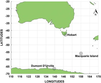
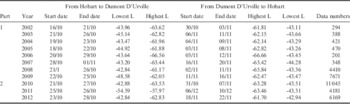
The MINERVE project acquired data during three cruises each summer from October to March, between Hobart (Tasmania, Australia, ~43°S) and Dumont D’Urville (Adélie Land, Antarctica, ~67°S) (Fig. 1). Only data from early summer is considered here, mainly in October and November; see Table I for dates and latitudes of each cruise used to establish (part 1) and validate (part 2) the model.
Regional map showing Hobart, Dumont D’Urville and Macquarie Island. Source: Google Earth.

Details of the MINERVE database. Part 1 was used to establish the model. Part 2 was used to validate the model. L=Latitude.

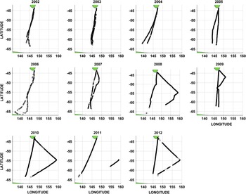
The cruise tracks (Fig. 2) every year cross all latitudes between Tasmania and Antarctica, although the presence of ice in the early summer prevents data collection south of ~63°S. Changes of longitude are primarily due to weather conditions; however, in some years (2008, 2010, 2011 and 2012), the ship had to go to Macquarie Island (55°S, 158°E) (Fig. 1).
Cruise tracks of the MINERVE project where data are during the first cruise every year.

Data and model
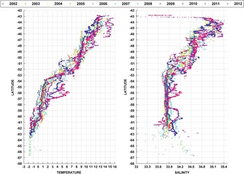
The MINERVE project provides data on surface water parameters from southern Australia to the sea ice edge north of Antarctica. The latitudinal distribution of SST and SSS (Fig. 3) shows cooling and freshening from roughly SST=2°C and SSS=35.1 near Hobart to ~-1.9°C (the freezing point) and 33.9 near 63°S. There is a substantial range in both SST and SSS at each latitude, associated with both the differences in cruise tracks (Fig. 2) and interannual variability.
Latitudinal distribution of temperature and salinity in the Southern Ocean south of Australia during the 2002–12 MINERVE project.

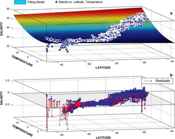
The surface fitting toolbox of MATLABTM was used to develop a model based on the MINERVE database of SST, SSS and latitude, φ. This toolbox performs multiple linear regressions between these three variables. This method provides good results for our purpose (Moussa et al. Reference Moussa, Benallal, Goyet, Lefevre, El Jai, Guglielmi and Touratier2015). We carried out the analysis for Part 1 of the database (2002–09), setting the degree of φ at 1 and the degree of SST at 2, resulting in the following function:
 $$SSS_{{mod}} \,{\rm =}\,a{\plus}b{\asterisk}{\rm \varphi }{\plus}c{\asterisk}SST{\plus}d{\asterisk}Lat{\asterisk}SST{\plus}e{\asterisk}SST^{2} ,$$
where the optimized values of coefficients were a=33.10000, b=-0.01257, c=0.103600, d=0.001929 and e=0.008504. The fitting surface and the residual plot are shown in Fig. 4.
Model suggested by the surface fitting toolbox. a. Dataset points and fitting surface. b. Residuals plot.

Three statistical measures were calculated to evaluate the model. Model error at each point in parameter space is defined as ei=Pi−Oi where e i is the error, P i (i=1..n) is the model-predicted value and O i (i=1..n) is the observed value. The root-mean-square error (RMSE; Willmott & Matsuura Reference Willmott and Matsuura2005) is defined as:
 $$RMSE= \left[ {{1 \over n}\mathop{\sum}\nolimits_{i=1}^n {e_{i}^{2} } } \right]^{{{1 \over 2}}}. $$
The mean absolute error (MAE) is based on the absolute value of each error estimate (Willmott & Matsuura Reference Willmott and Matsuura2005), i.e.
 $$MAE{\rm =} {1 \over n}\mathop{\sum}\nolimits_{i=1}^n {\!\mid\!e_{i} \!\mid}. $$
The mean bias error (MBE) is the simple average of individual error estimates:
 $$MBE{\rm =}{1 \over n}\mathop{\sum}\nolimits_{i=1}^n {e_{i} }. $$
The MBE indicates whether the average estimate is less than or greater than the observed values. The following measures were obtained for the modelled error in salinity: MBE=-3.01×10⁻¹⁴, MAE=0.0706, and RMSE=0.0958. The values for MBE and RMSE indicate that the model, in general, has a salinity accuracy that is comparable with satellite-derived SSS accuracy. However, some large values of e i are found in the far southern portion of the domain (Fig. 4b).
Results
Satellite-derived maps of SST were obtained from Moderate Resolution Imaging Spectroradiometer (MODIS) on the NASA Aqua satellite. Data are provided as daily averages with a spatial resolution of 4×4 km (http://oceancolor.gsfc.nasa.gov). For comparison with the MINERVE database, MODIS SST points corresponding as closely as possible in space and time to our in situ datapoints were selected.
Our statistical fit model (Eq. 1) was then applied to the satellite-derived SST and latitude φ to estimate SSS, and compare these values with in situ SSS data for part 2 data (2010–12) that were not included in the development of the model fit. The loss of satellite-derived SST data due to weather substantially reduces the number of points for comparison, from 21 395 to 4672 points.
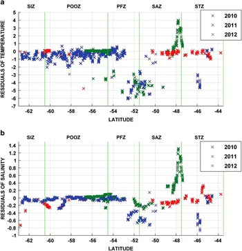
There is a mismatch between satellite and in situ SST around 48°S and 51°S (Fig. 5a). These errors are probably due to the calibration of the satellite instruments, which is rather complex. At the moment, there are four main calibration methodologies. The aim of these methodologies is to have a good accuracy over the globe; however, calibration can cause significant errors when satellite data are compared with specific local in situ data. Note that these errors appear in two fronts (explained in the following paragraph) which increase the difficulty for modelling for the satellite algorithms.
Salinity and temperature residuals (satellite to in situ data comparison). Residuals between a. satellite and observed temperature, and b. estimated and observed salinity.

The errors as functions of latitude (Fig. 5) are usually small but with some regions of large outliers. The study area was divided into three regions (Laika et al. Reference Laika, Goyet, Vouvé, Poisson and Touratier2009) representing five different hydrographic zones of the Southern Ocean (Rintoul et al. Reference Rintoul, Donguy and Roemmich1997):
-
1. The Sub-Antarctic Region (SAR) which it is composed of three zones:
-
a. The Sub-Tropical Zone (STZ) from -43.5° to -47.5°.
-
b. The Sub-Antarctic Zone (SAZ) from -47.5° to -51.5°.
-
c. The Polar Frontal Zone (PFZ) from -51.5° to -54.5°.
-
-
2. The Permanent Open Ocean Zone (POOZ) from -54.5° to -60.5°.
-
3. The Seasonal Ice Zone (SIZ) from -60.5° to -65°.
Table II shows all residuals by zone and for the whole study area.
Model testing results (2010–12).

MAE=mean absolute error, MBE=mean bias error, PFZ=Polar Frontal Zone, POOZ=Permanent Open Ocean Zone, RMSE=root-mean-square error, SAR=Sub-Antarctic Region, SAZ=Sub-Antarctic Zone, SIZ=Seasonal Ice Zone, STZ=Sub-Tropical Zone.
Model errors are larger in the SAZ and STZ than in the other zones. However, the error in the estimation of salinity is correlated with the difference between the in situ and the satellite temperature (Fig. 5a). That is, the large errors in SSS for some latitude ranges are caused by errors in satellite-derived temperature rather than in our regression model (Eq. 1).
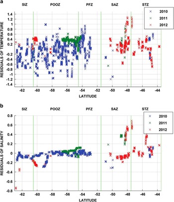
There is large mean bias between satellite and in situ temperature (Fig 5a), with MBE=-0.6952 (Table II). When outliers are removed, keeping only points where residuals are between +1 and -1.5, the new MBE is -0.2974. This bias is applied to satellite temperature data so that the MBE becomes zero. After testing the model, new residuals for salinity and temperature are smaller; compare Fig. 6 with Fig. 5, and Table III with Table II.
Salinity and temperature residuals after selecting process. Residuals between a. satellite and observed temperature, and b. estimated and observed salinity.

Model testing results after the selection process.

MAE=mean absolute error, MBE=mean bias error, PFZ=Polar Frontal Zone, POOZ=Permanent Open Ocean Zone, RMSE=root-mean-square error, SAR=Sub-Antarctic Region, SAZ=Sub-Antarctic Zone, SIZ=Seasonal Ice Zone, STZ=Sub-Tropical Zone.
Discussion
Satellite SST maps are available every day (with more or less points provided depending on the climatic conditions), at 4 km spatial resolution. The model we have established (Eq. 1) allows us to map SSS at the same resolution in the early summer in the Southern Ocean south of Australia. This spatial resolution is much finer than we can obtain from existing satellite salinity sensors on the Aquarius and SMOS satellites (~150 km and 50–100 km, respectively). The daily sampling of SST by satellites is much more frequent that either salinity satellite provides. The accuracy of our model, in salinity units (RMSE=0.116 for the entire region from 43oS to the ice edge near 63oS), is comparable to the cited accuracy of the satellite-derived values; therefore, our model may provide valuable information on SSS for temporal and spatial scales that cannot be resolved by the satellite-based salinity records. An additional source of error, when modelling SSS based on satellite-derived SST, is that the RMSE for satellite vs in situ SST is ~0.38oC (Table III); based on Eq. (1), this converts to ~0.1 in SSS.
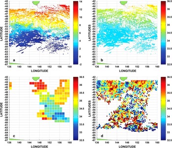
As an example of the potential value of our model, Fig. 7 compares a one day modelled SSS (Eq. (1) applied to satellite-derived SST data) with coarser estimates from SMOS and Aquarius. The differences between resolutions are clear. Note that SMOS data are provided as an average of at a minimum of three days.
Comparison of modelled sea surface salinity (SSS) using sea surface temperature (SST) with SMOS and Aquarius satellite data. a. Satellite SST in the Antarctic Ocean south of Australia on 25 October 2011. b. Modelled estimated salinity from a. c. Aquarius satellite image from 25 October 2011. d. SMOS three-day average satellite image from 25 October 2011 to 27 October 2011.

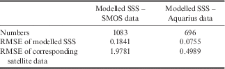
Table IV shows a pairwise comparison of modelled SSS with SMOS data and with Aquarius data using in situ data from 2011 to 2012 (Table I, part 2). The RMSE of our modelled SSS is much smaller than both SMOS and Aquarius data.
Comparison between modelled sea surface salinity (SSS) and two satellite products (SMOS and Aquarius).
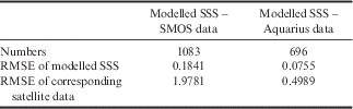
RMSE=root-mean-square error.
Conclusions
We have demonstrated the value of developing algorithms to relate SSS to satellite-derived SST, by providing the ability to map SSS at much finer spatial and temporal scales that can be resolved by existing salinity satellites, Aquarius (stopped on 17 June 2015) and SMOS. Furthermore, as these satellites have only been operating for a few years, the algorithm allows the extension of maps of SSS into time ranges for which no satellite maps of SSS are available. This approach can be further developed to determine SSS throughout the year, and to contribute to a broader range of applications including determination of surface density, air-sea exchanges, and estimation and analysis of air-sea CO2 fluxes.
Collecting more in situ data is the best way to improve our models; therefore, it is important that the MINERVE project remains active.
Acknowledgements
I would like to express my very great appreciation to all the persons who built and continue to provide accurate databases for the MINERVE project, and the IPEV (Institutpolaire français Paul Émile Victor) which provides the logistics framework, human resources, and technical and financial resources to the development of French research in the Polar Regions. I would like to thank NASA for providing satellite temperature images. I am particularly grateful for the MESRS (Ministère de l’Enseignement Supérieuret de la Recherche Scientifique) from Algeria which funded my PhD and gave me the opportunity to undertake research at the IMAGES laboratory. We are also grateful to the reviewers for their comments on the manuscript.
Authors contributions:
Mrs H. Moussa was involved in the conception and writing of the programs for the study. Dr F. Touratier supervised this PhD research and assisted with writing and revising this paper. Professor C. Goyet assisted with analysis of the data and provided ideas for the selection process which enabled the achievement of better results, and also participated in revising the article. Professor A. Poisson participated on the MINERVE project where we found our data, and also assisted with revising the article.