

Introduction
The completeness of the fossil record is an evident obstacle in paleontological studies. The state of preservation of a fossil has an impact on all subsequently applied analyses (Raup Reference Raup1972; Benton et al. Reference Benton, Dunhill, Lloyd and Marx2011). While deformation factors can be corrected for in a single specimen, analyses pertaining to a higher systematic scale and to clades’ macroevolutionary patterns, such as paleobiodiversity studies or phylogenetic analyses, have in the past often left that problem aside. However, studies of phylogeny and paleobiodiversity are both built upon the description and classification of individual specimens; without considering the completeness of these specimens, it is difficult to know how robust the results are. While the authors of phylogenetic analyses often acknowledged incompleteness by giving the percentage of missing data in their data matrices, studies into the effect of the completeness of specimens have only recently become widespread, and methodologies are inconsistent.
There have been many attempts to quantify the completeness of the fossil record based on various proxies. Many attempted to infer how sampling biases have impacted taxonomic richness, for example, by comparing proxies such as the number of fossiliferous formations, number of localities, or outcrop area to diversity curves (Benton et al. Reference Benton, Tverdokhlebov and Surkov2004; Fröbisch Reference Fröbisch2008; Barrett et al. Reference Barrett, McGowan and Page2009; Benson et al. Reference Benson, Butler, Lindgren and Smith2010; Benson and Upchurch Reference Benson and Upchurch2013). Recent studies have proposed that proxies for rock volume, such as the geographic spread or outcropping surface area, could be used and measured using geographic information systems and then compared with diversity curves (Smith and McGowan Reference Smith and McGowan2007, Reference Smith and McGowan2008; Mannion et al. Reference Mannion, Upchurch, Carrano and Barrett2011; Upchurch et al. Reference Upchurch, Mannion, Benson, Butler and Carrano2011; Dunhill et al. Reference Dunhill, Benton, Twitchett and Newell2012; Fröbisch Reference Fröbisch2013). The general conclusion reached by these studies is that geological sampling biases have an impact on short-term variation of diversity, mostly at a regional or local scale, although in some cases (e.g., Alroy Reference Alroy2010; Benson et al. Reference Benson, Butler, Alroy, Mannion, Carrano and Lloyd2016), an effect has also been noticed on large-timescale fluctuations of diversity.
In the last decade, multiple metrics focusing on the actual fossil specimens were proposed. These are measures of fossil completeness, state of preservation, and taphonomy in general. For example, Fountaine et al. (Reference Fountaine, Benton, Dyke and Nudds2005), Smith (Reference Smith2007), Beardmore et al. (Reference Beardmore, Orr, Manzocchi, Furrer and Johnson2012), and Benton et al. (Reference Benton, Ruta, Dunhill and Sakamoto2013), directly measured a specimen’s or taxon’s completeness and/or state of preservation. These methods essentially rate completeness according to a crude previously defined scale, for example, from 1 (fragmentary remains) to 4 (several complete skeletons) for Paleozoic and Mesozoic tetrapods in Benton et al. (Reference Benton, Ruta, Dunhill and Sakamoto2013). These scoring systems appeared to be very subjective and imprecise, and to overcome these issues, Mannion and Upchurch (Reference Mannion and Upchurch2010) proposed two more quantitative measures of completeness: the skeletal completeness metric (SCM) and the character completeness metric (CCM), to investigate the quality of fossil specimens of sauropodomorph dinosaurs (see below for details on these metrics). Recently, these methods have been applied to other vertebrate taxa, including Mesozoic birds, anomodont and pelycosaur-grade synapsids, ichthyosaurs, and pterosaurs (Brocklehurst et al. Reference Brocklehurst, Kammerer and Fröbisch2013; Walther and Fröbisch Reference Walther and Fröbisch2013, Reference Walther and Fröbisch2014; Brocklehurst and Fröbisch Reference Brocklehurst and Fröbisch2014; Cleary et al. Reference Cleary, Moon, Dunhill and Benton2015; Dean et al. Reference Dean, Mannion and Butler2016). Surprisingly, Cleary et al. (Reference Cleary, Moon, Dunhill and Benton2015) demonstrated that, in ichthyosaurs, the Beardmore’s skeletal completeness metric, cruder and quicker to assess, shows a highly significant correlation with the more detailed and time-consuming SCM, indicating that the choice of completeness metric may not affect the results to a great extent.
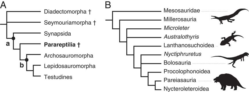
Nonetheless, for the present study, the more detailed completeness metrics of Mannion and Upchurch (Reference Mannion and Upchurch2010) are applied to Parareptilia, a major clade of early amniotes (Fig. 1A). This group first appeared in the late Carboniferous (Modesto et al. Reference Modesto, Scott, MacDougall, Sues, Evans and Reisz2015) and persisted until the end of the Triassic (Ruta et al. Reference Ruta, Cisneros, Liebrecht, Tsuji and Müller2011). Parareptiles comprise about 90 described species, being very diverse in terms of ecology and morphology. They include: one of the earliest groups of amniotes to have returned to the aquatic environment, the mesosaurids; some of the largest terrestrial vertebrates of the Permian period, the often-armored herbivorous pareiasaurs; the earliest known facultatively bipedal tetrapod, the bolosaurid Eudibamus (Berman et al. Reference Berman, Reisz, Scott, Henrici, Sumida and Martens2000); the rare and flat-skulled lanthanosuchoids; and several lizard-like and possibly fossorial forms such as millerettids and procolophonoids. Figure 1B shows the interrelationships of the individual parareptile groups.
A, Summary phylogeny of amniotes, based on Hill (Reference Hill2005). Highlighted nodes: a, Amniota; b, Diapsida. B, Summary phylogeny of parareptiles, based on Tsuji and Müller (Reference Tsuji and Müller2009). † indicates extinct clades. Silhouettes are from PhyloPic (Keesey Reference Keesey2015). From top to bottom: Mesosaurus tenuidens, Lanthanosuchus watsoni, Eudibamus cursoris (©Nobumichi Tamura CC BY-SA 3.0), and Scutosaurus karpinskii (public domain). Not to scale.
Parareptiles became the subject of a renewed attention in the 1990s because they were thought to include the lineage that gave rise to turtles; Eunotosaurus, procolophonoids, and pareiasaurs all having suggested as turtles’ evolutionary antecedents (Carroll Reference Carroll1988; Laurin and Reisz Reference Laurin and Reisz1995; Lee Reference Lee1995, Reference Lee1997). These hypotheses have been generally abandoned (deBraga and Rieppel Reference deBraga and Rieppel1997; Cao et al. Reference Cao, Sorenson, Kumazawa, Mindell and Hasegawa2000; Zardoya and Meyer Reference Zardoya and Meyer2001; Tsuji and Müller Reference Tsuji and Müller2009), although some recent studies have again suggested a close relationship of Testudines and Eunotosaurus (Lyson et al. Reference Lyson, Bever, Bhullar, Joyce and Gauthier2010). However, recent studies indicate that Eunotosaurus, which was traditionally considered a parareptile, actually represents a diapsid reptile in the process of developing an anapsid skull condition and is indeed closely related to the origin of turtles (Bever et al. Reference Bever, Lyson, Field and Bhullar2015). Independent of the origin of turtles, parareptiles are of great interest due to their great ecological diversity and because, through procolophonoids, they are one of the few clades that survived the most severe extinction event in Earth history at the end of the Permian. In this paper, we assess the completeness of the parareptile fossil record, comparing various metrics to examine different aspects of specimen completeness.
Methodology
Completeness Metrics
Mannion and Upchurch (Reference Mannion and Upchurch2010) introduced two quantitative completeness metrics, the SCM and the CCM, with two different implementations, respectively designated as SCM1 and CCM1 versus SCM2 and CCM2. The first implementation determines the completeness of only the most complete specimen of a taxon, while the second considers the completeness of all known specimens of this taxon. Here, only the second implementation is used, for two reasons: (1) it is considered to be more meaningful than the single-specimen approach (Mannion and Upchurch Reference Mannion and Upchurch2010), and (2) the variable importance attributed to different parts of the skeleton may complicate the definition of the most complete specimen.
The CCM reflects the amount of phylogenetic information available for a given taxon. It is based on the number of characters from a phylogenetic data set that can be scored for each taxon. In the original article by Mannion and Upchurch (Reference Mannion and Upchurch2010), the CCM was calculated by measuring the average number of characters referring to each bone in multiple matrices and by assigning the corresponding percentage to every bone actually present in the specimen. Brocklehurst et al. (Reference Brocklehurst, Upchurch, Mannion and O’Connor2012) improved the implementation of the CCM (hereafter, Brocklehurst’s implementation is called “CCMa”): the number of characters potentially coded on a given bone is obtained by counting the number of original characters referring to this bone in as many phylogenetic matrices as possible, unified in one single combined matrix with duplicate characters removed. Then the character completeness percentage for this bone is calculated based on the total number of characters in the matrix. For example, if a specimen has a humerus preserved, and this bone is referred to in 4 characters out of 10, then the specimen’s completeness is 40%. The sum of the percentages of all elements preserved gives the completeness of the taxon.
In a later study, Bell et al. (Reference Bell, Upchurch, Mannion and Lloyd2013) suggested a simpler method for calculating the CCM (hereafter referred as “CCMb”), which only requires access to cladistic matrices, and not to descriptions of specimens or the specimens themselves. In this approach, the ratio between the number of characters scored in a taxon and the total number of characters in the matrix is calculated for all matrices in which the taxon is included. The final completeness of the taxon is the average value from all matrices in which it is included. Here, we also calculated the completeness by dividing the total number of characters scored for the taxon by the total number of characters in all the matrices in which it is included. Correlation tests showed a very high correlation between these two methods (ρ=0.969, p<0.001), and so only the latter was employed.
Both CCMa and CCMb were compared in this study. The combined character list, required for the first approach (Mannion and Upchurch Reference Mannion and Upchurch2010), was built from three lists extracted from the most recent and exhaustive phylogenetic studies on parareptiles (Tsuji et al. Reference Tsuji, Müller and Reisz2012, Reference Tsuji, Sidor, Steyer, Smith, Tabor and Ide2013; MacDougall et al. Reference MacDougall, Modesto and Botha-Brink2013). In the second approach (Bell et al. Reference Bell, Upchurch, Mannion and Lloyd2013), 13 matrices were used: one of millerosaurians (Cisneros et al. Reference Cisneros, Rubidge, Mason and Dube2008), one of pareiasaurs (Tsuji Reference Tsuji2013), two of bolosaurians (Müller et al. Reference Müller, Li and Reisz2008; Falconnet Reference Falconnet2012), three of procolophonoids (Modesto and Damiani Reference Modesto and Damiani2007; Säilä Reference Säilä2008; MacDougall et al. Reference MacDougall, Modesto and Botha-Brink2013), and five general phylogenies of parareptiles (Reisz et al. Reference Reisz, Müller, Tsuji and Scott2007; Modesto and Reisz Reference Modesto and Reisz2008; Sues and Reisz Reference Sues and Reisz2008; Tsuji et al. Reference Tsuji, Müller and Reisz2012; Modesto et al. Reference Modesto, Scott, MacDougall, Sues, Evans and Reisz2015). These matrices were chosen because they were the most recent and because their association provided at least one value for each parareptile taxon. Older matrices were not included, since the more recent ones were often modified or expanded versions of these.
The SCM reflects how much of the skeletal material is preserved for a given taxon. Mannion and Upchurch (Reference Mannion and Upchurch2010) originally obtained the SCM by partitioning skeletons into several sections (e.g., “skull,” “hind limbs,” etc.) and then assigning roughly estimated percentages of how much of the skeleton these parts represented. As this method is prone to subjective approximations, Brocklehurst and Fröbisch (Reference Brocklehurst and Fröbisch2014) proposed an alternative method to implement the SCM. In their paper, a general morphological model was built for all pelycosaur-grade synapsids based on skeletal measurements: each bone was modeled as a simple geometric shape, like a cylinder or a prism, whose volume constituted a proportion of the skeleton (the latter being given by the sum of all shapes’ volumes).
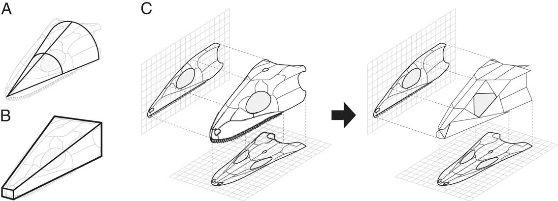
In this study, we used a modified version of Brocklehurst and Fröbisch’s method. First of all, rather than approximating long bones and the vertebral column as cylinders, which can only imprecisely give an account of the shape variety, these structures were modeled by hourglass-shaped volumes or truncated cones, which allows more accuracy. Furthermore, the calculation system of cranial completeness was revised. Brocklehurst (unpublished data) modeled the skull (including the mandible) as a cone divided into eight three-dimensional sections that were considered complete according to which skull bones were present or not (Fig. 2A). This method suffers from the lack of a precise quantification of the completeness of complex bone associations and still resorts to rough estimations of how complete the sections are.
Approximation models of skull volume. A, Cone model used in Brocklehurst et al. (Reference Brocklehurst, Kammerer and Fröbisch2013). B, Truncated pyramid model employed in the present study. C, Construction of the surface approximation model for the volume of skull bones, based on figures showing side and plan views.
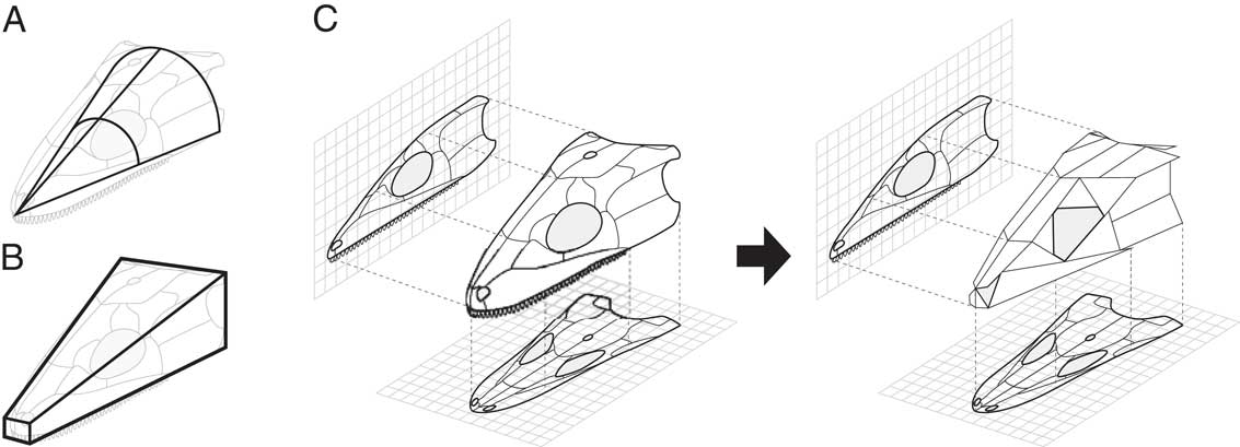
Here, instead of a cone, the skull (without the mandible) was modeled as half of a truncated pyramid, constrained by its length, occipital and snout widths, and occipital and snout heights (Fig. 2B), while the mandibles were separately modeled as two rectangular prisms. Then, the external surface of each cranial bone (rather than its volume) was estimated by assimilating the outlines of the bone to a simple geometrical shape such as a parallelogram, triangle, or ellipse (Fig. 2C). The proportion obtained by dividing this surface by the sum of all surfaces was reported as the estimated skull volume to calculate the volume of the bone. For example: the maxilla can be modeled as a triangle; if its surface is 10 cm2, and the sum of all cranial bones’ surfaces is 100 cm², then the maxilla is one-tenth of the skull surface, and its estimated proportion will therefore be one-tenth of the skull. All measurements for the surface estimation were carried out on figures showing the skulls in plan, occipital, lateral, and palatal views. This method, although still an estimate, is nonetheless more precise and less subjective than previous approaches.
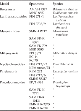
Another difference from the original method (Brocklehurst and Fröbisch Reference Brocklehurst and Fröbisch2014) is that we built several different geometric models instead of one, because the diversity in shapes and skeletal proportions among parareptiles (Fig. 1B) does not allow use of a single model for all taxa. Pareiasaurs, for example, have an entirely different Bauplan when compared with procolophonoids or mesosaurids. Thus, seven models were constructed for seven principal clades with distinct morphological characteristics (Supplemental Table 1). They were based on several specimens from different taxa; the list is detailed in Table 1. For groups with unknown skeletal elements, volumes of these missing parts were calculated based on the proportions found in the most complete and most morphologically similar model.
List of the specimens used to construct the skeletal models used for calculation of the SCM. Quotation marks refer to the name above.

Data Set
The study was carried out at the genus level. This choice was motivated by the fact that most parareptile genera are monospecific and most of the phylogenetic analyses were performed at the genus level as well. To include as many taxa as possible while avoiding synonymy issues, we extracted a list of valid parareptile genera from the latest and most exhaustive study on this group (Ruta et al. Reference Ruta, Cisneros, Liebrecht, Tsuji and Müller2011). Added to this list were: Abyssomedon (MacDougall and Reisz Reference MacDougall and Reisz2014), Contritosaurus (Ivakhnenko Reference Ivakhnenko1974), Delorhynchus (Reisz et al. Reference Reisz, MacDougall and Modesto2014), Erpetonyx (Modesto et al. Reference Modesto, Scott, MacDougall, Sues, Evans and Reisz2015), Feeserpeton (MacDougall and Reisz Reference MacDougall and Reisz2012), Obirkovia (Bulanov and Yashina Reference Bulanov and Yashina2005), and Phonodus (Modesto et al. Reference Modesto, Scott, Botha-Brink and Reisz2010). In the end, we considered 76 taxa of parareptiles. Mesosaurids were not included in the CCMb analysis because they were not scored as genera or species in any of the included phylogenetic studies but rather treated as a composite clade coding.
A matrix describing precisely which skeletal elements and how many of them are known for every genus was built. Descriptions of the specimens were extracted from the literature. To investigate completeness patterns through time, knowledge of the stratigraphic range of the genera was assembled. This data was downloaded from the Paleobiology Database (Uhen and Sessa Reference Uhen and Sessa2013); the data set may be considered complete as of December 2015.
Statistical Tests
CCM and SCM give a percentage value for each taxon (Supplementary Table 2). An average completeness was calculated for each Permian and Triassic stage (Fig. 3). The three curves (CCMa, CCMb, and SCM) obtained were compared with one another and to a generic diversity curve (Fig. 3D) with nonparametric correlation tests: Spearman’s rank correlation coefficient (Spearman Reference Spearman1904) and Kendall’s tau rank correlation coefficient (Kendall Reference Kendall1938). To correct for autocorrelation, the data were transformed via generalized differencing (McKinney Reference McKinney1990). Table 2A presents results of the tests obtained on the complete data set. To avoid exaggerated weight given to some taxa due to monogeneric diversity in five stages (Gzhelian, Asselian, Sakmarian, Ladinian, and Rhaetian), we also applied the correlation tests on a data set excluding these stages. Results obtained with this data set are presented in Table 2B.
Curves of completeness through time. A, CCM according to Brocklehurst et al.’s (Reference Brocklehurst, Upchurch, Mannion and O’Connor2012) method (CCMa). B, CCM according to Bell et al.’s (Reference Bell, Upchurch, Mannion and Lloyd2013) method (CCMb). C, SCM. The thick lines correspond to the mean value of completeness; dashed lines are the standard error ranges; gray circles are the scatter of completeness values in each stage. D, Generic diversity of parareptiles through time. The vertical gray line marks the Permian/Triassic boundary. x-Axis ages are in Ma. Abbreviations used for geological stages in this figure (and all following): Gzhelian (GZH), Asselian (ASL), Sakmarian (SKM), Artinskian (ATK), Kungurian (KUG), Roadian (ROD), Wordian (WOR), Capitanian (CAP), Wuchiapingian (WUC), Changhsingian (C), Induan (I), Olenekian (OLK), Anisian (ANS), Ladinian (LAD), Carnian (CRN), Norian (NOR), Rhaetian (RHA), and Carboniferous (CARB.). Color version online.

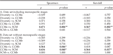
Results of the correlation tests. Asterisks show the significance level of the correlation as defined in the text. Bold numbers highlight significant correlations.

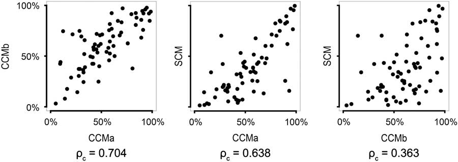
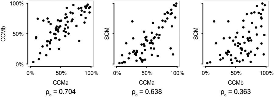
The correlation between metrics was also analyzed without taking the temporal dimension into account. Figure 4 shows the scatter plots of the three metrics in pairs. To depart from the natural correlation due to the three metrics quantifying the same information, we used Lin’s concordance correlation coefficient (Lin Reference Lin1989). Lin’s ρc measures the agreement between two variables. Values of this coefficient are also displayed in Figure 4.
Plotted values of the three completeness metrics in pairs. “ρc” is the result of Lin’s concordance correlation coefficient for each association.
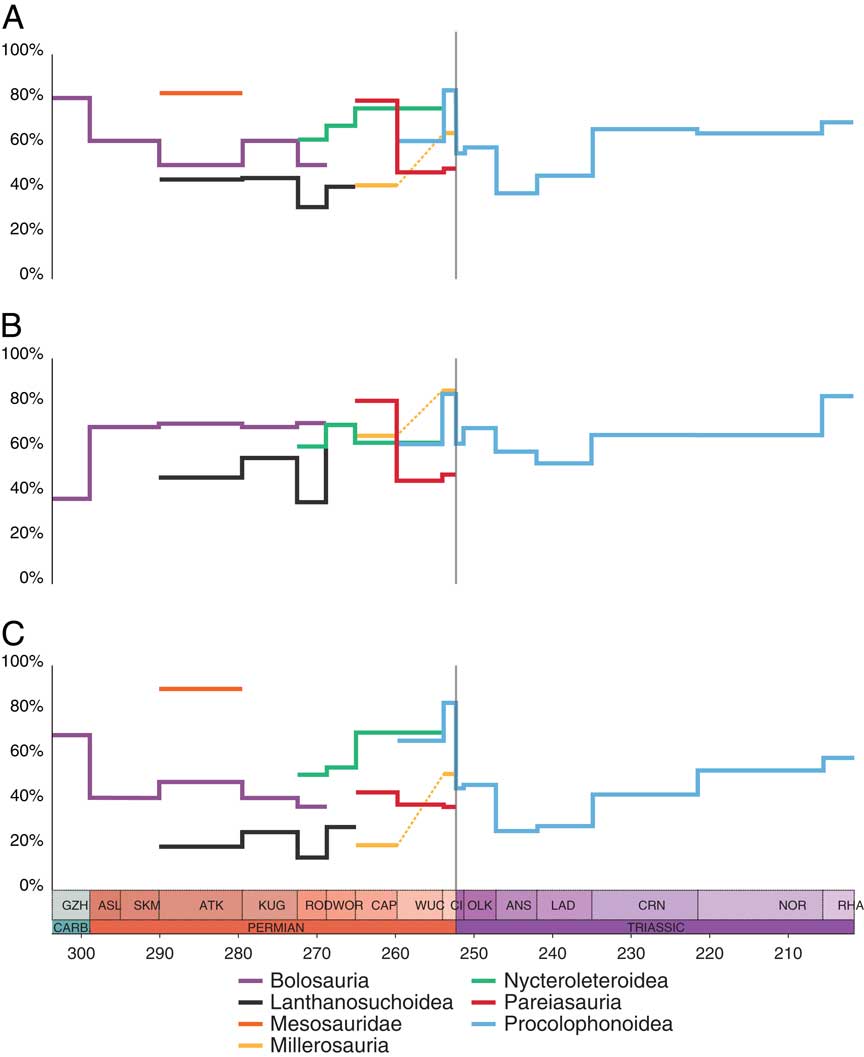
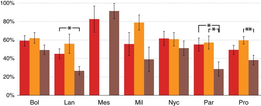
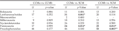
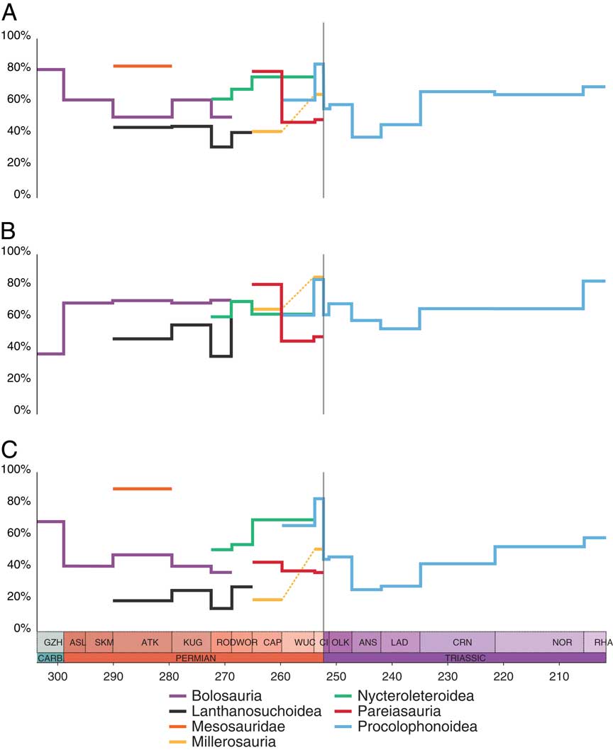
In addition to this global analysis of parareptile completeness through time, a study focusing on the completeness of the individual major parareptile clades was carried out. The average completeness observed in each group is shown in Figure 5. Given that the number of genera per group was always less than 30, the differences between the distributions were tested with nonparametric Mann-Whitney U-test (Mann and Whitney Reference Mann and Whitney1947); results are shown in Table 3. Finally, the variation of completeness through time within the groups is shown in Figure 6.
Completeness of each group through time. A, CCM according to Brocklehurst et al.’s (Reference Brocklehurst, Upchurch, Mannion and O’Connor2012) method (CCMa). B, CCM according to Bell et al.’s (Reference Bell, Upchurch, Mannion and Lloyd2013) method (CCMb). C, SCM. The thin dotted line in Millerosauria represents a gap in the fossil record of the group during the Wuchiapingian.
Average completeness for the three metrics for each clade. Left red bars (printed black) are the CCMa; middle orange bars (printed light gray) are the CCMb; right brown bars (printed dark gray) are the SCM. Error bars show the SEM. Brackets with stars show the significance of the difference between the two pointed metrics according to Mann-Whitney’s U-test (*, p<0.05; **, p<0.01). Abbreviations used: Bolosauria (Bol), Lanthanosuchoidea (Lan), Mesosauridae (Mes), Millerosauria (Mil), Nycteroleteroidea (Nyc), Pareiasauria (Par), Procolophonoidea (Pro). Color version online.
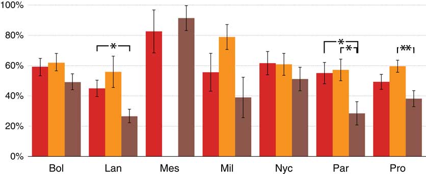
Results of the Mann-Whitney U-tests comparing the mean values of completeness for each group and each metric. Asterisks show the significance level of the difference between two means as defined in the text. Bold numbers highlight significant correlations.

All statistical analyses were carried out using R 3.1.0 (R Core Team 2016). The symbols representing the significance of a result in tables and figures are: * when p<0.05; ** when p<0.01.
Results
Completeness
The mean of the CCMa score of each time bin is 59% (Fig. 3A). The maximum (81%) is reached during the late Carboniferous (Ghzelian), then decreases (70%) during the latest Triassic (Rhaetian), and reaches a minimum (37%) during the early Middle Triassic (Anisian). The mean CCMa score is quite stable during the Permian and until the late Early Triassic (Olenekian), ranging between 55 and 64%, with the exception of the late early Permian (Kungurian) and late middle Permian (Capitanian), being 47% and 70% respectively. The mean CCMa does not change greatly at the Permian/Triassic boundary, but drops significantly in the Middle Triassic. After the overall minimum in the Anisian (37%), the CCMa increases only slightly in the Ladinian before reaching a plateau with values above 65% in the Late Triassic. The maximum CCMa of all taxa in each time bin (uppermost gray circles) is very high, with values consistently above 90% during the entire study interval, except during the early Permian (Sakmarian, Kungurian) and the Middle Triassic, with the lowest value (46%) in the Ladinian. The minimum completeness (lowermost gray circles) is quite low and stays below 40% from the Artinskian to the Norian, except during the Sakmarian (62%), Ladinian (46%), and the Carnian (42%), and drops below 20% from the Wuchiapingian to the Anisian.
The CCMb is more variable (Fig. 3B) but with a higher average mean value of 63% through time. The highest mean CCMb is reached in the Rhaetian (83%), with the second- and third-highest peaks in the Capitanian and the Wordian (76% and 75%, respectively). The lowest mean CCMb values are recorded in the Gzhelian (38%) and the Wuchiapingian (51%). Mean CCMb varies between these peaks and troughs, with a plateau around 58% during the Permian from the Artinskian until the Roadian and a plateau around 66% during the Late Triassic (Carnian, Norian). Mean CCMb increases across the Permian/Triassic boundary. The maximum CCMb of all taxa in each time bin (uppermost gray circles) is again very high with values consistently above 80% and is more stable than the CCMa curve; it is only interrupted in the Ladinian with a minimum value of 54%. The minimum (lowermost gray circles) is quite variable, but mostly stays below 40% and in the Wuchiapingian and Changhsingian is even below 10%. There are three time intervals in the early Permian (Assilian–Sakmarian), middle Permian (Wordian–Capitanian), and Middle/Late Triassic (Ladinian–Carnian) with high minimum values above 50%.
The SCM is overall lower than the two CCM curves (Fig. 3C), with an average mean value of 45%. A maximum mean SCM of 69% is reached in the Ghzelian, with a second peak of 59% in the Rhaetian. The overall minimum of 26% occurs in the Anisian. After substantial variation from the Sakmarian until the Kungurian, the mean SCM is fairly stable above 40% from the Roadian to the Olenekian across the Permian/Triassic boundary. After this, mean SCM drops to a trough during the Anisian and Ladinian before rising back to late Permian levels, and thereafter continues to increase throughout the Late Triassic to a Rhaetian peak. As in the CCMa, the maximum SCM value of all taxa in each time bin (uppermost gray circles) is quite stable and high with values above 80% during the entire study interval, with the exception of the troughs in the Sakmarian, Kungurian, and Middle Triassic. The minimum SCM (lowermost gray circles) is very low and consistently under 20%, except during the Sakmarian, Ladinian and Rhaetian.
Correlation Tests and Concordance Coefficient
Table 2 shows the results of the correlation tests comparing the three completeness metrics and the generic diversity, based on curves with (Table 2A) and without (Table 2B) time bins containing only one genus. In both cases, it appears that none of the completeness metrics are significantly correlated with diversity, using either Spearman’s or Kendall’s tests. Including monogeneric stages, comparison of the metrics only shows a highly significant correlation between the SCM and the CCMa for both Spearman’s ρ (ρ=0.671, p=0.006) and Kendall’s τ (τ=0.567, p=0.002) tests. When monogeneric time bins are excluded, the correlation between CCMa and SCM is still significant for both tests: Spearman’s ρ (ρ=0.636, p=0.040) and Kendall’s τ (τ=0.564, p=0.017). In addition, a new significant correlation between CCMa and CCMb is highlighted, but only with Spearman’s ρ (ρ=0.564, p=0.046).
Figure 4 presents plotted values of completeness for the three metrics in pairs. Despite showing an important scatter, the association of CCMa and CCMb on one hand and CCMa and SCM on the other hand seems to follow a more or less linear relationship. On the contrary, the scatter in CCMb versus SCM is too substantial to support a close relationship. These visual inferences are supported by Lin’s concordance correlation coefficient. Results show a stronger agreement between CCMa and CCMb (ρc=0.704), and between CCMa and SCM (ρc=0.638), than between CCMb and SCM (ρc=0.363).
Completeness within Parareptile Clades
From the histogram of the mean completeness by clade (Fig. 6), it appears that the CCMb is always higher than the two other metrics, except in mesosaurids (which lack a CCMb value, as they are always included in the phylogenies as a family) and the nycteroleteroids. However, the fact that the CCMb values are above the others is not sustained by the statistical tests (Table 3). In lanthanosuchoids, the highest value is the CCMb, but there is only a significant difference between the CCMa and the SCM (U=31, p=0.041). For mesosaurids, there is no significant difference between the CCMa and the SCM. For millerosaurians and nycteroleteroids, there is no significant difference between any of the three metrics. In pareiasaurs, both CCMs strongly differ from the SCM. Procolophonoids are marked by a very significant difference between the CCMb and the SCM, but there is no difference between the CCMa and the SCM. Finally, mesosaurids have the highest completeness values in all metrics.
Completeness within Clades through Time
The temporal variation in completeness for each individual clade is shown in Figure 5. Parareptile completeness in the Triassic is only driven by procolophonoids, the only parareptile clade to survive the end-Permian mass extinction. Most notably, and in contrast to the overall pattern when considering all parareptiles, procolophonoid completeness drops in all three metrics across the Permian/Triassic boundary but only reaches an overall minimum in the Middle Triassic. While the different metrics do not give exactly the same results, they do show similar patterns within each clade. For example, lanthanosuchoids show an increasing completeness from the Artinskian to the Kungurian, decreasing in the Roadian to a trough lower than in the Artinskian, and finally increasing again in the Wordian, but with substantially different levels in each metric. The completeness of pareiasaurs consistently decreases between the Capitanian and the Wuchiapingian, then reaches a plateau, slightly increasing (CCMa and CCMb) or decreasing (SCM) in the Changhsingian. In millerosaurians, the Changhsingian completeness value is higher than the Capitanian for all metrics (they are only present in these two time bins).
Discussion
Parareptile Completeness
Figure 3 shows that the completeness of parareptiles through time is consistently high. None of the completeness curves show any great excursions from the mean value. In addition, the minor peaks and troughs that are visible do not correspond to any high or low values of taxic diversity (Fig. 3D). The correlation tests find no significant correlation between generic diversity and any of the three metrics (Table 2). This shows two things. First, there is no evidence of a Lagerstätten effect in parareptiles. If a parareptile-bearing deposit was exceptionally rich and complete, there would be a temporally coincident peak in both completeness and diversity. As maximum values of completeness are not linked to high taxic richness here, this is not the case. Second, low completeness values not being associated with peaks of diversity suggests that most parareptile genera are not defined based on fragmentary material. Therefore, the likelihood of great synonymy issues is quite low. This interpretation is reinforced by the mean completeness of parareptiles through time (45% for the SCM, 59% for the CCMa, 63% for the CCMb) being consistently high compared with those measured in other tetrapod clades, namely sauropodomorph dinosaurs (37–40%, Mannion and Upchurch Reference Mannion and Upchurch2010), Mesozoic birds (37%, Brocklehurst et al. Reference Brocklehurst, Upchurch, Mannion and O’Connor2012), and pelycosaur-grade synapsids (35–40%, Brocklehurst and Fröbisch Reference Brocklehurst and Fröbisch2014), whereas fossil specimens of anomodonts were found to be very complete (74%, Walther and Fröbisch Reference Walther and Fröbisch2013, Reference Walther and Fröbisch2014).
Regarding correlation between the three metrics, results differ depending on whether time stages with monogeneric diversity are included or not (Table 2). The main differences when monogeneric bins are not included is a significant correlation appearing between CCMa and CCMb for Spearman’s ρ (ρ=0.564, p=0.046). It could also mean that these five bins were extreme values, whose impact is exaggerated by the fact that they represent only one genus. By excluding them, less distorted information is measured in the correlation test. The results of Lin’s concordance correlation coefficient (Fig. 4), which does not depend on the time series, support the correlations found by the tests when monogeneric time bins are excluded.
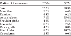
The two character completeness curves (Fig. 3A,B) are significantly and strongly correlated (Table 2) and have a strong agreement (ρc=0.704). This shows that, despite different protocols, the two methods measure the same signal. In contrast, only the CCMa is significantly correlated with the SCM, with a strong agreement (ρc=0.638), whereas none of the statistical tests indicates a significant relationship between the SCM and the CCMb (Table 2), and the agreement is low (ρc=0.363), despite the strong correlation between the latter and the CCMa. This could be due to the fact that the phylogenetic character matrices used to calculate the CCMb include many matrices intended to examine a specific clade, while matrices examining a broader range of taxa form the character list used in the CCMa. In a clade-specific phylogenetic matrix, the nature and the number of characters is implemented from the amount of available material in the group, so there already is a sorting of the studied elements, possibly leading to higher estimations of the group’s CCMb value. Although the CCMa and the SCM both weigh each portion of the skeleton differently (Table 4), the difference between them is dampened by several factors. First, the combined matrix used in the CCMa was constructed to attribute a percentage of completeness to each bone; every skeletal element is therefore represented, potentially differing from some of the matrices used for the CCMb. Moreover, both the SCM and the CCMa are implemented from the same list of the bones known for each taxon. Apart from some differences (for the SCM, every single skeletal element is considered, even in bilateral symmetrical bones, whereas the type of bone is only marked as present or absent for the CCMa), the two metrics are based on the same descriptive data.
Average percentages of completeness attributed to main portions of the skeleton for the CCMa and the SCM.

Figure 3 shows examples of how some patterns present in both CCMa and SCM are not found in the CCMb. For example, the Kungurian holds the lowest values of CCMa and the SCM in the Permian, while the curve shows a plateau for the CCMb. This may be driven by the bolosaurians, which have a higher CCMb than SCM and CCMa (Fig. 6). Calculation of the CCMb includes two bolosaurian-focused matrices (Müller et al. Reference Müller, Li and Reisz2008; Falconnet Reference Falconnet2012) in addition to the general matrices on parareptiles. In these matrices, the bolosaurian genera are scored for almost all characters, as the matrices are mostly based on cranial characters visible in the majority of bolosaurians, even though the number of skeletal elements preserved in these taxa is low (indicated by the low SCM score). While these factors explain the correlations between the completeness curves through time, other parameters must be taken into account to understand the completeness values of the individual parareptile clades (Fig. 6). As described above, the CCMb always holds the highest values, except in nycteroleteroids and mesosaurids (for which the CCMb could not be calculated), but once again, this is not always significant according to the statistical tests (Table 3). Furthermore, the relationships between the three metrics for each clade are not always the same and need to be considered in light of the respective fossil record of each individual group.
Bolosaurians, millerosaurians, lanthanosuchoids, and procolophonoids each have a higher CCMb than either of the other two metrics (Fig. 6). For the first three of these clades, and to a lesser extent for procolophonoids, very little postcranial material is known or at least incorporated in the current phylogenetic data sets. Thus, the phylogenetic matrices focus on cranial characters by necessity, which tends to artificially inflate the CCMb, since a poorly preserved postcranium will not have a substantial negative effect.
In nycteroleteroids and pareiasaurs, the two CCM metrics have similar values, and the SCM is lower, this difference being statistically significant in pareiasaurs. In this case, the difference between the SCM and the CCMa is likely due to the fact that a specimen can receive a complete CCMa score even if the entire skeleton is not preserved. For example, only one complete humerus is required to score characters relating to the humerus, so a fossil preserving a complete humerus will receive the complete CCMa score for the humerus. In contrast, the SCM score will reflect the fact that only one of the two humeri is actually preserved. Pareiasaurs and nycteroleteroids are known from incomplete skeletons and not only from skulls (Supplementary Table 2). Several elements of the postcranial skeleton, including limbs, girdles, and the vertebral column, are known, but not entirely, and often the paired elements are not both preserved.
Mesosaurids are the only group to have a lower CCMa than SCM. Two of three genera, Mesosaurus and Stereosternum, are known from virtually complete skeletons. Their CCMa values are slightly lower than their SCM values but still very high (97.1% and 96.4% for the CCMa vs. 99.7% and 99.6% for the SCM, respectively). In contrast, the gap between the SCM and the CCMa in the third genus, Brazilosaurus, is large enough to explain the discrepancy: this genus has a CCMa of 54.3% while its SCM is 74.9%, a difference of more than 20%. Brazilosaurus is known only from a skull, some limb fragments, and several almost complete vertebral columns (including the tail) with ribs. In the CCMa, the vertebrae and ribs together attribute 5.0% of the completeness to the genus, whereas in the SCM, the presacral ribs alone are 20.1% of the volume of the skeleton, and the presacral vertebrae 17.8%. In contrast, the completeness of the skull is significantly more important in the CCMa than in the SCM (Table 4).
Mesosaurs are also the parareptile clade with the highest completeness in all metrics. The explanation is probably both ecological and taphonomical. Mesosaurids are aquatic animals; as previously mentioned they are one of the earliest groups of amniotes to readopt an aquatic lifestyle. Living in an aquatic environment with a high sedimentation rate, they were more likely to be preserved and in better condition than terrestrial parareptiles. This may also explain why their fossils are much more abundant; 30 specimens of Mesosaurus alone have been described according to the Paleobiology Database (Uhen and Sessa Reference Uhen and Sessa2013), but the total number of unpublished specimens in collections is much higher, in the hundreds.
Nevertheless, this link between an aquatic lifestyle and a high completeness does not seem to affect another parareptile clade comprising aquatic animals, the lanthanosuchoids. Indeed, their completeness results are some of the lowest among parareptiles (Fig. 6). Several hypotheses can be formulated to explain this phenomenon. First, not all lanthanosuchoids are regarded as aquatic; Feeserpeton, Acleistorhinus, and Colobomycter (together representing half of the lanthanosuchoid genera included in this study) are only known from skulls and were probably terrestrial. This can partly explain why the overall completeness of lanthanosuchoids is so low. But although the three other genera are generally considered to be aquatic, they too are only known from skulls (except Lanthaniscus, which also includes some vertebrae). Actually, no paleoecological study has ever been carried out on lanthanosuchoids. Those assumed to be aquatic are designated as such because their flat and broad skulls resemble those of stegocephalians (Ivakhnenko and Kurochkin Reference Ivakhnenko and Kurochkin2008). Their way of life is not known well enough to confidently state whether their environment should have had an impact on their completeness or not.
In addition, body size does not seem to have an effect on the completeness of parareptile fossils. For example, pareiasaurs, some of the heaviest and largest tetrapods of the late Permian, have completeness values similar to the contemporary procolophonoids (Fig. 6), which are small, lizard-like animals. Body-size effects on preservation have previously been observed in other groups (Brocklehurst et al. Reference Brocklehurst, Upchurch, Mannion and O’Connor2012), but here the context is different. First, and as mentioned above, the fossil record of parareptiles does not include any apparent Lagerstätten, which would have increased the number of well-preserved small animals. While it might seem intuitive that large and robust skeletons are less likely to be destroyed than smaller ones, this study and others (e.g., Fara and Benton Reference Fara and Benton2000; Brocklehurst et al. Reference Brocklehurst, Upchurch, Mannion and O’Connor2012; Cleary et al. Reference Cleary, Moon, Dunhill and Benton2015) indicate the relationship may not be so simple.
Methodological Implementations
A number of different implementations of the CCM have been used in the various studies on diverse clades. Here, we examine the impact of using the different CCM methods on our interpretations of the fossil record. The comparison of the different completeness metrics highlights some general issues. First, it appears that the CCMa results can be distorted by the fact that this method does not take into account the state of preservation of the individual bones. With the CCMa, each bone receives a percentage completeness score corresponding to the number of characters that refer to it. But it is assumed that, if a bone is present, every character can be scored on this bone. As the characters generally refer to detailed anatomical structures, and not to the entire element, a particular aspect of morphology may not necessarily have been preserved even if the bone was. The CCMa does not take into account the fact that a bone may be preserved, but not in such a way that allows all characters to be scored. Because of this, it could be argued that the CCMa tends to overestimate specimen completeness.
There is another consequence resulting from the way the combined character list is constructed. Some of the characters in the list may refer to bones that are present in some clades but not others. For such a group, the completeness is biased toward lower values: highly complete specimens may receive a lower score, since a bone they never possessed will be marked as missing. The importance of this effect obviously depends on the percentage of completeness attributed to the absent bone. In this study, osteoderms are a good example of this phenomenon. Among parareptiles, only pareiasaurs have osteoderms, but these structures represent 2.8% of the CCMa score. The groups that do not have osteoderms will therefore have a maximum completeness of 97.2%. The more characters are referring to such elements and the more complete the specimen, the greater the underestimation of completeness. This effect is insignificant in this study due to the small percentage of characters relating to osteoderms. But in other groups or in the case of sexual dimorphism, it may be an issue and should be considered in future studies where this is applicable.
The CCMb, meanwhile, is more prone to underestimate completeness. In the phylogenetic matrices, especially in those including a great variety of taxa, some characters refer to structures that may not be naturally present in every clade and will be scored as question marks, as if that portion of the anatomy were missing. This therefore increases the number of unscored characters and decreases the completeness. However, the results of the correlation tests (Table 2) and of the agreement coefficient (Fig. 4) indicate that the two CCM methods are measuring the same signal. Moreover, despite the fact that CCMa should overestimate completeness while CCMb underestimates it, CCMa is not consistently higher than CCMb (Figs. 3, 5). We can therefore conclude that the different issues highlighted above are not significantly affecting the results.
Ultimately, the most accurate method, the one that has the least biases, is the SCM. Indeed, the only source of imprecision is the resolution of the geometric models. But although reliable, this method suffers from being relatively time-consuming to implement. Particularly, the construction of the individual skeletal models requires access to multiple specimens or accurate descriptions for relevant measurements to be made. The choice is therefore to be precise by using those models or to be fast by employing subjective values, as initially proposed by Mannion and Upchurch (Reference Mannion and Upchurch2010). Interestingly, Cleary et al. (Reference Cleary, Moon, Dunhill and Benton2015) showed in their study on ichthyosaurs that using less precise, easier to implement methods does not substantially change the results. The CCMb is extremely easy to implement, as it only requires phylogenetic data matrices, which are readily available from publications; but it is the most biased method of the three. CCMa is more precise, but also more time-consuming with respect to data assemblage in the form of a list of elements, and direct access to specimens is required. In addition to the slightly different focus of each metric, these aspects of speed versus accuracy need to be taken into account when choosing between these metrics and their applicability to individual fossil clades.
Conclusion
Our completeness study of Parareptilia, one of the major clades of amniotes, demonstrates that their fossil record, with respect to the quality of specimens, is of high quality and with particularly high values of character completeness when compared with most previously studied vertebrate groups, indicating that the available data are a solid basis for phylogenetic analyses and further macroevolutionary studies. There is no effect of body size on completeness, whereas ecology seems to have an impact on preservation. Our study shows that although different implementations reflect slight variations in the results, the differences do not seem to affect our interpretation of the parareptilian fossil record. It is nevertheless important to keep these issues in mind when examining the completeness of a clade; for example, when calculating the CCM one must consider the intended purposes of the original character matrices used, which will have influenced the character selection and, by extension, the completeness scores.
Acknowledgments
We are first of all grateful to Johannes Müller for discussions and providing access to specimens of Emeroleter levi, and likewise to Daniela Schwarz, Curator of Fossil Reptiles, Fossil Birds and Ichnofossils at the Museum für Naturkunde Berlin, for access to specimens of Mesosaurus. We also wish to thank Christian Kammerer for his constant support and his helpful comments and our many colleagues at the Museum für Naturkunde Berlin. Finally, we are grateful for the reviewers taking the time to read through the text and provide constructive comments. This study was financially supported by the Languedoc-Roussillon region, the University of Montpellier, and a Sofja Kovalevskaja Award, which was awarded by the Alexander von Humboldt Foundation and donated by the German Federal Ministry for Education and Research. This is Paleobiology Database official publication number 261.
Supplementary Material
Data available from the Dryad Digital Repository: http://dx.doi.org/10.5061/dryad.b5k79