1. Introduction
The Magnetized Liner Inertial Fusion (MagLIF) concept (Slutz et al. Reference Slutz, Herrmann, Vesey, Sefkow, Sinars, Rovang, Peterson and Cuneo2010) being studied at the Sandia National Laboratories Z-facility (Rose et al. Reference Rose, Welch, Madrid, Miller, Clark, Stygar, Savage, Rochau, Bailey and Nash2010; Savage et al. Reference Savage, LeChien, Lopez, Stoltzfus, Stygar, Artery, Lott, Corcoran, Curry and Oliver2011) utilises a large $\mathcal {O}(20\,{\rm MA})$ current to compress a cylindrical beryllium tube, known as a liner, containing a pure deuterium fuel. Prior to compression, a pre-imposed $\mathcal {O}(10\,{\rm T})$
 axially oriented magnetic field is applied (Rovang et al. Reference Rovang, Lamppa, Cuneo, Owen, McKenney, Johnson, Radovich, Kaye, McBride and Alexander2014) and the fuel is preheated by a multi-kilojoule laser (Rambo et al. Reference Rambo, Smith, Porter, Hurst, Speas, Adams, Garcia, Dawson, Thurston and Wakefield2005, Reference Rambo, Schwarz, Schollmeier, Geissel, Smith, Kimmel, Speas, Shores, Armstrong and Bellum2016). As the liner is accelerated inward due to the high magnetic pressure generated by the drive current, the fuel is quasi-adiabatically heated through $P\,{\rm d}V$
 work and the magnetic flux is compressed, aiding in the trapping of charged fusion products. When the thermal pressure in the fuel becomes great enough to balance the magnetic drive pressure, the implosion stagnates with ion temperatures $T_{\text {ion}} \approx 3$
 keV, fuel radial areal densities $(\rho R)_{\text {fuel}} \approx 2\,{\rm mg}\,{\rm cm}^{-2}$
 and several kilotesla magnetic fields (Gomez et al. Reference Gomez, Slutz, Jennings, Ampleford, Weis, Myers, Yager-Elorriaga, Hahn, Hansen and Harding2014).
In order to assess the resulting plasma conditions and morphology generated in MagLIF experiments, a variety of spatially and spectrally resolved x-ray diagnostics have been developed and fielded (Hansen et al. Reference Hansen, Gomez, Sefkow, Slutz, Sinars, Hahn, Harding, Knapp, Schmit and Awe2015; Harding et al. unpublished observations). Here we focus on a variety of single and dual spherical crystal x-ray imager (SCXI) capabilities (Harding et al. unpublished observations) that include the possibility for spectral filtering to focus on spectral regions containing information that continues to shape our understanding of quantities such as mix, liner areal density and morphology of the stagnated fuel. Significant insight would be gained by understanding the physical conditions and associated well-resolved spatial structure produced across our entire experimental database. However, this has remained a challenge due to significant expertise and manual labour required to process and analyse the images. As a result, it has generally only been feasible to compare images from a small number of experiments (Harding et al. unpublished observations; Ampleford et al. unpublished observations; Glinsky et al. Reference Glinsky, Moore, Lewis, Weis, Jennings, Ampleford, Knapp, Harding, Gomez and Harvey-Thompson2020). While the qualitative insights gained in these studies have proven critical, developing automated processing routines and model-independent quantitative metrics to describe and compare structure of different spectral regions or even different experimental realisations would significantly alleviate this constraint. Such a capability would open the possibility for large-scale experimental studies to highlight structural similarities and differences that may otherwise go unnoticed due to the need for an expert to sort through a high volume of rich image data collected on Z.
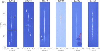
SCXI data spanning from early to recent MagLIF experiments and employing different imager modalities results in a significant variety of structural and instrument-induced features arising for example from emission from the fuel and liner, background emission, statistical noise, spatial fiducials and image plate damage as demonstrated in figure 1. These features make it difficult to utilise traditional unsupervised image analysis tools such as edge and peak detection via filtering algorithms to process the data without significant user input. Deep-learning-based algorithms have recently demonstrated success in overcoming these types of challenges in the processing, analysis and emulation of image and spectroscopic data in a variety of high energy density and fusion physics applications (see, for example, Ferreira et al. Reference Ferreira, Carvalho and Fernandes2018; Anirudh et al. Reference Anirudh, Thiagarajan, Bremer and Spears2020; Kluth et al. Reference Kluth, Humbird, Spears, Peterson, Scott, Patel, Koning, Marinak, Divol and Young2020; Thiagarajan et al. Reference Thiagarajan, Venkatesh, Anirudh, Bremer, Gaffney, Anderson and Spears2020; Simpson et al. Reference Simpson, Mariscal, Williams, Scott, Grace and Ma2021; Kustowski et al. Reference Kustowski, Gaffney, Spears, Anderson, Anirudh, Bremer, Thiagarajan, Kruse and Nora2022). To address this issue, we introduce a mostly automated processing pipeline utilising a combination of supervised machine learning and unsupervised rules-based algorithms to register images and remove background signal detailed in § 2. We process $N_{\text {scans}} = 139$ images gathered across $N_{\text {exp}} = 67$
 different experiments utilising a variety of different SCXI diagnostics. In §§ 2.1–2.4, we detail the full image processing pipeline beginning with preprocessing of the scanned image plates and proceeding to automated segmentation, registration, rotation and background subtraction. While an attempt was made to develop a completely automated end-to-end approach that would produce the desired registered and background subtracted images, our pipeline does require minimal human input. In particular, although we have a large number of images relative to available human resources, our image database would still be considered to be in the small data regime relative to what is required to train typical machine learning pipelines. Our data also exhibit a number of (rarely occurring) pathologies and artifacts which we describe in detail throughout the text. As a result, careful hand labelling paired with significant data augmentation would be required to enable end-to-end approaches for our data. Therefore, we have chosen to balance the requirement of human input (§ 2.1) and synthetic data models (§ 2.2.1) with the need to hand label images to achieve full automation without reference to synthetic data models. We opted for the former, as the latter of the two would effectively require completing the desired segmentation task manually. The pipeline we present may be considered as a mostly automated labelling algorithm that could be used to aid in training end-to-end tools in the future. Finally, in § 3, we provide a statistical assessment over the ensemble of images for the noise statistics in our images, the signal-to-noise ratio (SNR) and background signal. These results provide support for and guidance of assumptions made in statistical inference methods and synthetic dataset generation for machine learning tasks and general analysis of MagLIF stagnation images.
MagLIF stagnations images exhibit complex structures induced by a variety of factors. The white dashed line on the image for shot, for example, indicates a fiducial that was fielded, whereas the white arrows on $z2851$ , $z2948$
 and $z3019$
 indicate extended emission structures. In the first two cases, this structure appears to arise from the outer surface of the liner, whereas in the case of $z3019$
 the emission is likely from some other source, e.g. cathode emission. $z3087$
 exhibits lower contrast due to a lower signal-to-noise ratio. $z3240$
 shows two regions indicated by red arrows, where plate damage occurred so that signal in and around that region is obscured. Note also the variety of structures seen. For example, $z2948$
 shows a shorter emission column, corresponding to fielding of a $7.5$
 mm tall liner as opposed to the standard $10$
 mm tall target, $z3087$
 exhibits large-scale axial brightness variation, $z3019$
 and $z3240$
 were a dielectric coated targets (Ampleford et al. unpublished observations) and exhibit more uniform emission columns, and both $z3240$
 as well as $z3500$
 show more detail in the column structure due to the use of a significantly higher-resolution spherical crystal imaging configuration (Harding et al. unpublished observations; Lewis et al. unpublished observations).

2. Image processing pipeline
In order to make our work repeatable and extendable, we developed a mostly automated image processing workflow, the components of which are detailed in this section. The full pipeline is composed of four major stages. The first step detailed in § 2.1 is an initial data preprocessing stage. The resulting preprocessed image is passed through to the second stage which is image segmentation via a convolutional neural network (CNN) presented in § 2.2. This segmentation provides information that is useful for the third stage discussed in § 2.3, which conducts refinement of both the original image and mask via translation and rotation to centre the stagnation column and align it vertically. Finally, a low-order polynomial model is fit to the background portion of the image using a cross-validation procedure discussed in § 2.4.
2.1. Preprocessing experimental images
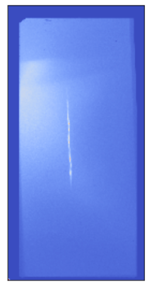
The raw experimental image data are made available as an image plate scan, an example of which is shown in figure 2. From the figure, it should be apparent that the image plate may be fielded and scanned in one of a handful of gross orientations indicated by the notched corner (upper-left) along with the possibility of a small random rotation $\mathcal {O}(\pm 1^{\circ })$ of the plate in the scanner. This notch allows determination of the orientation relative to the actual experiment provided it is identifiable. Notch identifiability is one of the first pathologies that may be encountered in our dataset, with some image plates apparently lacking a notch, or having duplicate notches. Also note that the object of interest, namely the stagnation column, occupies only a fraction of the plate, and may be present near the centre or edge of the plate.
Example of an image plate scan. Note the dark border indicating that the scan area is larger than the image plate. Also note the bright background feature starting on the left side of the image plate. The notch in the upper left corner of the image plate indicates orientation, and must be recorded as metadata by the user.

Although we originally attempted to fully automate our image processing pipeline, we found it necessary to balance rarely occurring pathological features and small dataset size relative to those required for training machine learning pipeline with the need for the user is required to perform a small number of simple manual tasks as we now detail. First, it must be determined whether an image is eligible for analysis. An image may be ineligible if there is significant damage to the image plate obscuring the stagnation column, the scan of the plate is badly saturated or no strand is seen in the scan. Next, for eligible images, the user records the gross orientation of the image plate (i.e. notch position) used to ensure proper final image orientation. Finally, the user identifies a region of interest (ROI) containing the strand. Note that figure 2 shows that the scan contains off-plate regions which appear as zero-valued pixels. In addition, bright artifacts can appear at the edge of the image plate which can exceed the signal strength coming from the stagnation strand. The very high dynamic range resulting from this relatively small number of pixels can make identifying and cropping the strand difficult in some cases. As a result, we use an approach similar to sigma-clipping outlier rejection in order to make the cropping task significantly easier for the user. The algorithm is given as follows.
(i) Compute $\bar {X} = (X-\mu )$
 where $X$ is the image scan, $\mu = 1/N_{\text {pixels}} \sum _{p \in \text {pixels}} X_{p}$ is the average pixel value, and $N_{\text {pixels}}$ is the number of pixels.
(ii) Compute $\sigma = \sqrt {{\sum _{p \in \text {pixels}} \bar {X}_{p}^2}/{N_{\text {pixels}}}}$
.(iii) If $|\bar {X}_p| > f \sigma$
where $f >1.0$ is a user-specified multiplier which defines a condition for outliers, set $\bar {X}_p = \text {sign}(X_p)f\sigma$.(iv) Repeat steps (i)–(iii) until a maximum number of iterations $N_{\text {max}}$
is met or convergence occurs, i.e. $\sigma _i-\sigma _{i+1} < \text {tol}$, with $\text {tol}$ being a user-specified tolerance, and $i$ indicates the particular iteration of the algorithm.


For our purposes, we find $f=3.0$ , $N_{\text {max}} = 10$
 , and $\text {tol} = 10^{-3}$
 to be sufficient for our entire experimental image database. The user then specifies coordinates of the upper-left corner of a crop window of fixed spatial dimensions, again requiring only that the ROI contain the strand. The image orientation and crop coordinate metadata is saved for use in the subsequent processing stages.
Before moving on to discuss the second stage of our processing pipeline, image segmentation, it is worth highlighting a few points. First, it is a well-demonstrated feature of CNNs that results are generally insensitive to small translations and rotations in the input images (when selecting appropriate network architecture and/or including augmented training data including samples having some rotational offset) (Goodfellow, Bengio & Courville Reference Goodfellow, Bengio and Courville2016). As a result, the current need for a human-in-the-loop to preprocess by cropping is not expected to affect the accuracy of the segmentation network presented in § 2.2.2. Second, as a supervised learning algorithm, the segmentation network will require training data. For this purpose, we use an analytic model containing plasma conditions and geometry first discussed in Knapp et al. (Reference Knapp, Glinsky, Schaeuble, Jennings, Evans, Gunning, Awe, Chandler, Geissel and Gomez2022) and further detailed in § 2.2.1 to create synthetic images to train the network. The training data will only approximate the complexities of our experimental data. In particular, for the case of high dynamic range resulting from a small fraction of pixels containing much higher or lower signal value than the strand as mentioned previously, our training data do not appropriately capture the variance in the experimental data. As a result, we find that the segmentation network, trained only on synthetic data, performs much better on our experimental data without any need for transfer learning if we apply the above sigma-clipping algorithm to experimental images before computing the strand segmentation map. In more detail, the need for outlier rejection may be understood as follows. As is typically required for most machine learning algorithms, an appropriate normalisation must be applied to data before passing the data to the algorithm. We apply a min–max normalisation that scales pixel brightness to lie in $[0,1]$ before being fed into the segmentation network (see § 2.2.2). This will result in a significant and atypical compression of the brightness values associated with the strand, making identification more difficult for cases where bright artifacts or plate damage are present. The sigma-clipping directly addresses this issue by removing such gross outliers in an automated fashion.
2.2. Deep-learning-based image segmentation
Automating image registration, rotation and background subtraction requires knowledge of what constitutes the stagnation column in our images. Features such as the presence or lack of emission from the cold liner, axial brightness variation, differences in apparent helical structure, debris/damage, slowly varying background, the occasional fielding of a partially obscuring spatial fiducial and noise make broad application of unsupervised approaches to this task challenging without case-by-case algorithm tuning. In this section, we present the details of a CNN which can successfully segment our experimental images into strand and background despite this wide variety of experimental features.
2.2.1. Synthetic data model
In order for a CNN to learn a binary segmentation of SCXI images into stagnation column and background, labelled training data must be provided. Data for this task are automatically generated using a static model for the deuterium plasma comprising the fuel column, which was originally developed to validate axially resolved Bayesian inferences of fuel conditions for MagLIF experiments (Knapp et al. Reference Knapp, Glinsky, Schaeuble, Jennings, Evans, Gunning, Awe, Chandler, Geissel and Gomez2022). The model can be roughly considered to be composed of a geometric portion, a physics portion and a synthetic diagnostic portion, all of which are described shortly along with details of parameter sampling for generating training data. We note that the model presented here allows not only for the creation of synthetic continuum emission SCXI data but can also be used to generate synthetic multi-channel pinhole camera images. We plan to utilise this model to address multi-channel data in a future publication. Furthermore, the use of this model allows us to automatically generate labelled datasets of arbitrary size for training. This avoids the need to provide hand-labelled experimental data and circumvents issues that would likely result from an experimental database of insufficient size to be used for training and validating such a model in any case, at least without significant data augmentation steps.
The geometric portion of the model provides for a parametrised spatial dependence of plasma conditions. The spatial structure allows for an arbitrary number, $s$ , of helical strands, which, for simplicity, we fix to be $s=2$
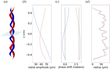
 . The general spatial structure of the model is shown in the first column in figure 3. Spatial strand coordinates are defined parametrically via the axial coordinate, $z$
 , which is zero at the mid-plane of our helical strands, as


The helical wavenumber is given by $k_s = 2 {\rm \pi}/\lambda _s$ , where $\lambda _s$
 is the helical strand wavelength, specifying the helical pitch. In the above, $A_s(z)$
 is a radial excursion amplitude allowed to vary over the axial extent according to the polynomial expansion

with $A$ being an overall constant multiple setting the length scale for the radial excursions and $A^i_{s,\zeta }$
 being polynomial coefficients that allow the radial excursion extent to vary slowly over the axial extent of the strand. The second column of figure 3 shows an example of the radial excursion amplitude vs axial coordinate. There is also a slowly varying phase factor, $\phi _s(z)$
 , that smoothly modulates the axial strand wavelength, which is expanded in Legendre polynomials as

where $L_i(z/Z)$ is the $i{{\rm th}}$
 -order Legendre polynomial, with $Z$
 setting a length scale over which we want the Legendre polynomials to evaluate in the interval $[-1,1]$
 . Here $Z = 5.75$
 mm is chosen, corresponding to a domain slightly larger than half the strand sizes typically observed in our stagnation images. In (2.5), the $p^i_{\varGamma,s}$
 are coefficients chosen so that $\phi _1(z)$
 fluctuates approximately zero and $\phi _2(z)$
 fluctuates approximately ${\rm \pi}$
 as shown in the third column of figure 3. Note that, henceforth, we refer to the strand $s=1$
 as the reference strand.
Example of one possible 3D structure from the geometric helical model, with the $s=1$ ‘reference strand’ shown in blue. (a) A surface plot demonstrating the radial excursion amplitude, relative phase and strand radii of the two strands versus height. The light blue plane indicates the mid-plane $z=0$
 . (b) The radial excursion amplitude ($A_s(z)$
 in (2.1)–(2.4)). (c) The axially varying phase shift of each strand. Note that the reference strand is centred around zero radians, whereas the $s=2$
 strand is centred around $\phi _s(z) \approx {\rm \pi}$
 . (d) The radius of the helical strand versus height. Note that the difference between the two strand radii is parametrised by the strand radius ratio parameter $\bar {r}_s(z)$
 described in the main text.

Before moving to the physics portion of the model, we define the remaining geometric parameters which are used in the physics portion. First, there is a function that will be applied later to physical and geometric conditions to constrain the axial extent of the fuel and provide additional axial fluctuations to these parameters according to a super-Gaussian profile given by

where $c$ denotes different ‘channels’, in particular, the strand radius, fuel temperature, fuel pressure, mix fraction and liner areal density (see, e.g., (2.12), (2.14) and (2.16)) to which the function h$^c(z)$
 is applied as detailed shortly. In the above, $\delta ^c(z)$
 is a function which randomly modulates the axial envelope, $\sigma = 2H/3$
 , where $H$
 sets the axial scale length for the strand, and $\xi$
 determines how rapidly the axial roll-off occurs. The factor of $2/3$
 in the relation of $\sigma _H$
 with $H$
 is so that $H$
 corresponds to a full width at half maximum when $\xi =1$
 . In the current implementation,

where $\delta ^c_0$ sets the scale for the amplitude of fluctuations and $\mathcal {U}_{[a,b]}(z)$
 ($\text {log}\mathcal {U}_{[a,b]}(z)$
 ) denotes a uniform (log-uniform) random number in the interval $[a,b]$
 chosen at each axial position. There are two final geometric parameters. The first is a strand radius scale $r_0$
 that sets the scale for the radial extent of temperature profiles at each axial position. The second is a strand radius ratio parameter $\bar {r}_s(z)$
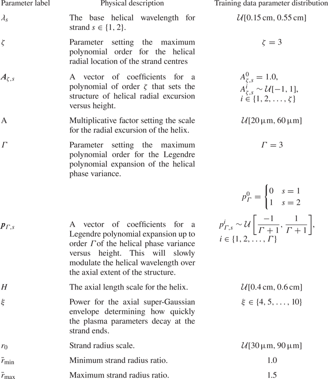
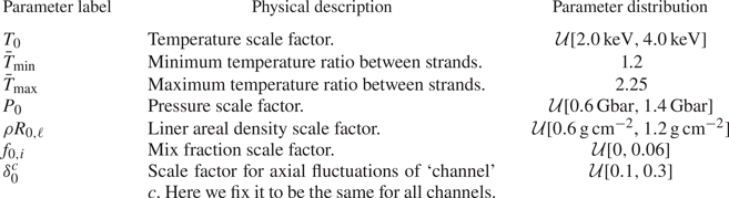
 which sets the difference in temperature profile radii of the strands. These last two parameters are only explicitly used in the physics model, and so are discussed in more detail in the following. For reference, the geometric model parameters along with a short physical description of their purpose are presented in table 1 along with the distribution from which those parameters are sampled for generating training data for the segmentation network.
Geometric parameter summary.

We now discuss the physics portion of the model which specifies the spatial dependence of the plasma conditions such as electron temperature, thermal pressure and mix. In what follows, the parametric dependence of the helical strand centres $x_s$ and $y_s$
 on the axial coordinate $z$
 is suppressed to save space. The electron temperature profile of the plasma is given by a sum of gaussian profiles for each of the strands as

At each axial position $z$ , the spatial temperature profile for strand $s$
 is given by

In the above, $N_s$ is the number of helical strands (here $N_s=2$
 ). The other functions appearing in (2.9) are


where $\bar {\ast }_{\text {min}(\text {max})}$ indicates the minimum (maximum) value of the associated sampling distribution, $T_0$
 is a parameter setting the overall temperature scale of the plasma and $\sigma _{T,s}(z)$
 determines the radius for each strand's Gaussian profile. For (2.13), $r(z) = r_0 h^r(z)$
 , with an example of the resulting strand radii shown in the rightmost column of figure 3. We assume that each horizontal slice of the plasma is isobaric so that the pressure is

The plasma is also allowed to have a uniform mix fraction of atomic species $i$ which varies axially as

For our synthetic images, we specify the laser entrance foil material, Kapton, to constitute the mix species, with the remaining fraction of atomic species being the background deuterium. Finally, we assume a liner areal density that will contribute to filtering the continuum emission from this plasma when computing synthetic diagnostics. Currently, we only allow the liner areal density to vary along the axial coordinate according to

We summarise the interpretation of the different physics model parameters in table 2 for convenience. We note that, in generating image ensembles, thresholding is applied to the temperature, pressure, linear areal density and strand radius to ensure that none of those quantities falls below $10\,\%$ of the corresponding specified scale parameter. This is a simple fix to avoid issues with random sampling that can cause unphysical negative values of the corresponding thresholded quantities as well as removing the potential for division by zero, but may contribute to artifacts in the synthetic image data as discussed in § 2.2.2.
Physical parameter summary.

In order to compute synthetic x-ray images, we must evaluate the emissivity from this plasma. To do so, we compute the time-integrated emissivity of the plasma assumed to be emitting uniformly into a solid angle of $4 {\rm \pi}$ including liner opacity, which, after suppressing spatial dependence, is given by (Ma et al. Reference Ma, Patel, Izumi, Springer, Key, Atherton, Benedetti, Bradley, Callahan and Celliers2013; Epstein et al. Reference Epstein, Goncharov, Marshall, Betti, Nora, Christopherson, Golovkin and MacFarlane2015)

The factors appearing in (2.17) that have not already been described are the frequency-dependent liner opacity $\kappa _\nu$ , the emissivity of each atomic species $j_i$
 , the burn duration here assumed to be uniform with $\tau _b = 2$
 ns and the free–free Gaunt factor ($g_{\text {FF}}$
 ). Evaluating the Gaunt factor in the high-temperature and high-photon-energy limit, $k_BT \gg \chi _H$
 with $\chi _H =13.6$
 eV being the hydrogen K-shell ionisation energy and $h\nu > k_BT$
 , respectively, where $k_B = 1.6022 \times 10^{-19}\,{\rm J}\,{\rm eV}^{-1}$
 , one may obtain (Epstein et al. Reference Epstein, Goncharov, Marshall, Betti, Nora, Christopherson, Golovkin and MacFarlane2015)

Assuming an optically thin plasma with negligible line emission, we may further write the emissivity as a sum of free–free ($j_i^\text {ff}$ ) and bound–free ($j_i^\text {fb}$
 ) emissivities


In the above, $Ry=13.6$ eV is the Rydberg constant, $A_\text {ff} = 2 \times 10^{-32}$
 J$^{3/2}$
 cm$^3$
 s$^{-1}$
 eV$^{-1}$
 is the free–free emission coefficient and $A_\text {bf} = 4 \times 10^{-31}$
 J$^{5/2}$
 cm$^3$
 s$^{-1}$
 eV$^{-1}$
 is the bound–free emission coefficient. Assuming equilibrated electron and ion populations ($T_e = T_{i} = T$
 ) and an ideal gas equation of state provides

with $\langle Z \rangle = \sum _i Z_i f_i$ being the average charge of the plasma. Utilising (2.18)–(2.22) and assuming that the plasma is isobaric at each axial position, we may rewrite (2.17) as

where

with $j_D$ being the emissivity of deuterium.
Using the emissivity, $\epsilon _\nu$ , we are able to compute synthetic SCXI data by utilising a Radon transform along an axis perpendicular to the $z$
 -axis, which maps a function $f(x,y,z):\mathbb {R}^3 \to \mathbb {R}$
 to a function $\mathcal {R}_{\hat {\alpha }}f(\bar {x}): \mathbb {R}^2 \to \mathbb {R}$
 defined on a plane containing the unit vector on the two-dimensional sphere, $\hat {\alpha } \in S^2$
 by integrating $\epsilon _\nu$
 along lines perpendicular to $\hat {\alpha }$
 . The Radon transform of a function $f(x,y,z)$
 is given by

where for each $\bar {x}$ the integral runs over the solution locus of $\boldsymbol {x} \boldsymbol {\cdot } \hat {\alpha } = \bar {x}$
 , and ${\rm d}A$
 is the surface area measure on a plane containing $\hat {\alpha }$
 . Note that here we are using $\bar {x}$
 to represent the two-dimensional Euclidean coordinates on a plane containing $\hat {\alpha }$
 . Also note that for our purposes, $\hat {\alpha }$
 will be restricted to the $x$
 –$y$
 plane and may be parametrised as $\hat {\alpha } = (\cos \theta,\sin \theta,0)$
 with $\theta$
 specifying the view angle. In that case, we may write the intensity of the synthetic image along a particular view angle, $I_\theta (\bar {x})$
 according to

Note that the expression contains a term, $\textit{R}_\nu$ , accounting for the reflectivity of the spherical crystal, and $\varPi (\bar {x})$
 representing the point-spread function for the optical system, assumed here to be Gaussian.
Before proceeding to use this model to train a convolutional network to segment the strand from the background, we pause to make several observations that may be of use in future work. First, note that the terms $\delta ^c(z)$ allow for axial variation of various parameters. However, the amplitudes are selected uniformly at random for each height from $[-\delta ^c_0,\delta _0^c]$
 as specified by (2.7). It is possible to impose smoothness in a variety of ways, such as using a Gaussian process to sample a variation function along the axial coordinate with amplitude determined by $\delta ^c_0$
 and a specified correlation length scale $\ell _0^c$
 . Extending this further, one could enforce correlations between different quantities. In our implementation, the point-spread function $\varPi (\bar {x})$
 will smooth out to some extent the noisy structure resulting from uniform random sampling in $\delta ^c(z)$
 , and for the purposes of this paper, the precise sampling approach is unimportant as we will see from the good performance of the segmentation network developed in the next subsection.
2.2.2. Segmentation CNN
We now apply the synthetic image model from § 2.2.1 in order to create a dataset to train a CNN to segment an image into strand and background. To do so, we begin by generating $N_\text {base} =1000$ images using the sampling distributions for each parameter as listed in tables 1 and 2. Provided the rather large parameter space indicated by tables 1 and 2, this might appear to be a small number of training samples. However, we apply a data augmentation step to obtain a factor of $10$
 more training samples. Furthermore, the task of segmenting an image is much simpler than other tasks one could train a machine learning algorithm to perform (e.g. inverting images to obtain the image geometric and physical parameters as in Glinsky et al. Reference Glinsky, Moore, Lewis, Weis, Jennings, Ampleford, Knapp, Harding, Gomez and Harvey-Thompson2020). More complex tasks typically require more training data. As we show, the obtained network does not overfit on validation data and performs well on experiments, justifying the use of this relatively small training dataset.
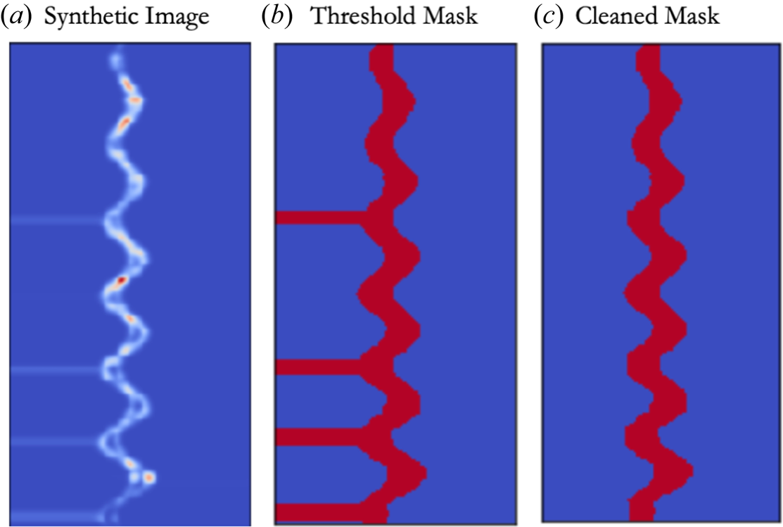
The masks indicating pixels corresponding to the strand are computed as the set of pixels taking on value greater than or equal to $20\,\%$ of the peak intensity, with a 2-pixel-wide expansion of the mask along each axis after thresholding. As indicated briefly in the previous section, thresholding physical parameters of the modelled plasma in conjunction with computing the Radon transform for synthetic image generation can result in an artificial striping structure in some of the computed images and masks demonstrated for a particular instance in figure 4. For our purposes, we consider this to be useful, because it may actually serve to help the convolutional network to ignore any off-strand features such as the cold-liner emission structures that are sometimes observable in our SCXI data as long as we are careful to remove the corresponding structures from the training data masks. Thus, we do not attempt to address the underlying issue here, but instead apply a cleaning algorithm to the resulting masks. This is achieved via a simple line-by-line scan that searches for the start of a horizontal stripe at the image edges and uses a nearby stripe-free region to compute the new mask edge.
(a) The training data from the synthetic model discussed in § 2.2.1, which can exhibit artificial horizontal banding. (b) Computing a simple mask by thresholding retains these artificial structures, and may result in poor performance on our experimental data. (c) After applying a simple cleaning procedure, the artificial structures are removed from the mask.

In order to increase our training dataset size and encourage the segmentation network to be robust to features that might arise in experimental data, we apply a set of several random data augmentation steps with $10$ different permutations applied to each of our original $1000$
 images, resulting in a total of $N_\text {augmented}=10\,000$
 images in our final dataset. The augmentation proceeds as follows. First, with probability $p_{\text {fid}} = 0.25$
 , a multiplicative ‘fiducial’ is applied

The synthetic fiducial is placed at a random height, $z_\text {fid}$ , between $10\,\%$
 and $85\,\%$
 of the image height, and serves to suppress pixels in a horizontal Gaussian band of random width, $\sigma _\text {fid}$
 , between $1\,\%$
 and $10\,\%$
 of the image height. This is meant to approximate the effect of fielding a spatial fiducial in experiment, which obstructs part of the emission, thereby creating an identifiable artifact that can be used to obtain an absolute position of the emission structure. Unfortunately, this can result in the mask to become disconnected, which may bias the registration algorithm discussed in § 2.3. The above augmentation and additionally serves to make our segmentation less sensitive to axial brightness variation. After (possibly) applying a synthetic fiducial, with probability $p = 0.25$
 we include a term to minimise the effect of large-scale brightness variation of the strand via multiplication by a step-like function

where $\boldsymbol {x} = (x,z)$ , $g_0$
 sets the minimum of the step-like function and $\boldsymbol {\aleph }$
 sets the direction and width over which the step-like function drops from $1$
 down to $g_0$
 . Subsequently, the image and mask are simultaneously rotated by the same random angle between $[-5^{\circ },5^{\circ }]$
 and then translated identically by a random amount between $\pm 25\,\%$
 in the $x$
 and $\pm 5\,\%$
 in the $z$
 directions, respectively. Experimentally, such translations and rotations occur due to both the original orientation of the image plate as fielded in the experiment as well as its orientation in the scanner.
In our experiments, we often see a slowly varying background, which, lacking coherence with respect to the signal arising from the strand, is expected to be additive (i.e. no optical interference effects will occur). As an additional augmentation step, we add a slowly varying background given by

to the image. In (2.29), $x$ and $z$
 are normalised by the corresponding image dimension, and allowed to take values in $[-1,1]$
 , $b_{n,m}$
 are sampled from $\mathcal {U}[-1,1]$
 and $b_0$
 sampled from $\mathcal {U}[0.01,0.3]\times \max _{\bar {x}}(I_\theta (\bar {x}) )$
 , whereas the order is chosen at random from $\text {order} \in \{1,2,3\}$
 with probability of selection for each order given by $p_\text {order} = [0.25,0.5,0.25]$
 . Note that a priori, we do not have quantitative information about the expected form or distribution of the background in experiment. Such an analysis is the primary goal in § 3. That said, low-degree polynomials are an obvious first choice to approximate the background, and the value of $b_0$
 was chosen to allow the background to range from between $1\,\%$
 and $30\,\%$
 of the peak intensity, which appears sufficient for the segmentation task to perform well on experimental images. Finally, normally distributed random noise is added to the synthetic image with a standard deviation equal to $10\,\%$
 of the original image peak amplitude. The resulting images are min–max scaled (scaled so that pixel values lie within $[0,1]$
 ) before use in training and validating the segmentation network described in the next paragraph.
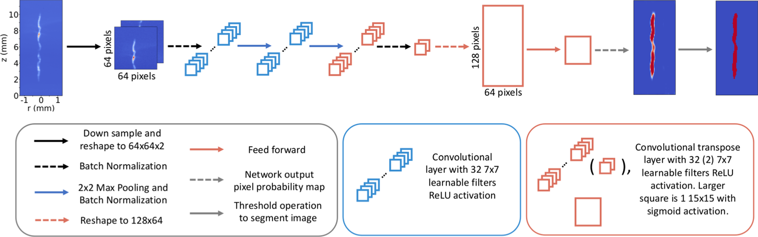
We now train a CNN to produce a pixel probability map indicating the probability $p \in [0,1]$ that a given pixel belongs to the stagnation strand. The architecture of this network is shown in figure 5. In performing this study, alternate sets of hyperparameters (e.g. learnable filter bank sizes and number of layers) were explored, with filter bank size having the largest effect. It was found that $7\times 7$
 filters were the smallest size that resulted in drastically outperforming smaller $3 \times 3$
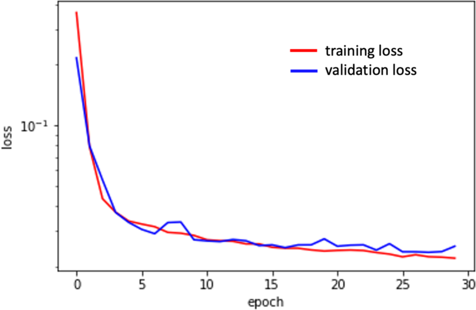
 filters we initialised the architecture with on both training and validation datasets. For learning network parameters, the augmented dataset is split into 70 %, 15 % and 15 % for training, validation and additional behaviour and performance testing, respectively. The network is constructed using the Keras package in Python with a tensorflow backend. The network is trained over 30 epochs with a batch size of 64 using Keras’ default ‘adam’ gradient descent optimiser (Kingma & Ba Reference Kingma and Ba2017) with a binary cross-entropy loss function (Bishop Reference Bishop2006) and Glorot uniform initialisation (Glorot & Bengio Reference Glorot and Bengio2010) of the network weights. We note that the network contains $N_\text {params} \approx 110\,000$
 trainable parameters, significantly larger than the number of training samples. However, the convolutional structure significantly regularises the network, and we do not see evidence of over-fitting as indicated by the comparison of the loss function on the training and validation data shown in figure 6.
Diagram of the image segmentation network architecture.

The binary cross-entropy loss function versus training epoch computed over the training data (red) and a hold-out validation dataset (blue). The close agreement between loss computed on the training and validation datasets is a good indicator that the network generalises well to unseen data and that over- and under-fitting have been effectively avoided.

The output of the convolutional network is a probability map, with each pixel taking on a value in $[0,1]$ . Denoting this output probability at the pixel in the $i$
 –$j$
 position as $P_{i,j}$
 , we can convert this into a mask, $\mathcal {M}_{i,j}$
 , by thresholding at a fixed probability value

We note that in our datasets, roughly $10\unicode{x2013}20\,\%$ of the pixels in a given image will belong to the stagnation column. As a result, pixel classification is inherently an imbalanced-class problem (Johnson & Khoshgoftaar Reference Johnson and Khoshgoftaar2019). In order to encourage the mask to include the entire strand, we set the threshold probability to be a fairly low value, $p_\text {thres} = 0.1$
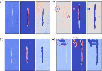
 . In addition, as noted in § 2.1, the experimental images are sigma-clipped and then min–max scaled before passing to the network to be segmented. Several randomly selected examples of the generated pixel probabilities and segmented images from experiment are demonstrated in figure 7. The results generally indicate excellent performance as seen in figures 7(a)–7(c), with only the most extreme cases of excessive background or image plate damage causing artifacts in the segmentation as demonstrated in figure 7(d). It is, in principle, possible to either modify our synthetic training data to capture these types of features, or to use transfer learning with labelled experimental data to make our network less sensitive to these anomalies. However, the volume of our experimental datasets being roughly 100 images rather than tens or hundreds of thousands or more, we chose to simply allow for a minimal human-in-the-loop presence during the refinement step described in § 2.3, recording all relevant metadata for reproducibility, to mitigate the influence of imperfect masking in the small number of extreme cases.
Computation of mask probabilities works exceptionally well when transferring the network trained on synthetic data to our experimental images. Even in the small number of cases where significant plate damage was observed as indicated by the red ellipses in the left column of (b,d), the strand is successfully identified. The inclusion of additional off-strand probability indicated by red ellipses in the centre column of (b,d) does somewhat reduce the effectiveness of the automated refinement procedure discussed in § 2.3. However, as long as the strand is effectively contained within the mask, slowly varying background subtraction performed in § 2.4 is expected to work effectively even if some background is falsely identified as belonging to the strand.

2.3. Automated image refinement
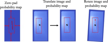
When comparing and assessing images, it is often desirable to utilise metrics that are relatively insensitive to translation and rotation. However, depending on the task, it may still be important to properly register images. Unfortunately, in general, no absolute spatial fiducial is available in our images. Despite this, it is reasonable to attempt to register the images based on gross features such as strand location and tilt angle to avoid complicating our interpretation of image metrics. We achieve this by using the pixel probability maps $p_{i,j}$ to perform mostly automated registration with an opportunity for user intervention in the rare event that mask probability computation exhibits anomalies.
The registration algorithm begins by computing the centre of probability, $\boldsymbol {p}_\text {cm}$ , and probability inertia tensor $I_{\alpha,\beta }$
 as


where $\boldsymbol {x}_{i,j}$ is the $i$
 –$j\text {th}$
 location (in integer pixel coordinates), and $\alpha,\beta$
 index whether the $i\text {th}$
 or $j\text {th}$
 coordinate value is to be taken. From $I_{\alpha,\beta }$
 we compute an angle by taking the eigenvector $\boldsymbol {w}$
 with the largest eigenvalue and compute $\theta _{\boldsymbol {w}} = \arctan {w_z/w_x}$
 . This gives the angle of the strand long axis with respect to the $x$
 -axis of the image. Next $\boldsymbol {p}_{\text {cm}}$
 and $\theta _{\boldsymbol {w}}$
 are used to translate and then rotate the image to centre and vertically align the stagnation column as indicated in figure 8. Note that, where needed, the pixel probability map is zero padded to perform any necessary rotations and translations. At this stage, the user is allowed to intervene if an extreme case results in poor registration. As an example, the image in figure 7(d) has a significant artifact caused by plate damage that will significantly affect registration. Windowing out the artifact results in good registration. When a problem arises, the user may choose one of the following.
(i) Perform the full routine described previously using a smaller windowed portion of the probability map to remove artifacts.
(ii) Perform only the centre-of-probability translation in the event that the strand was already nearly vertically aligned.
In order to ensure fully reproducible results, these choices are saved in an associated metadata text file.
Once the fuel–background segmentation probability maps are obtained, computation of the centre-of-probability and ‘probability inertia tensor’ can be used to centre the strand and rotate into the principle coordinate frame to align the strand vertically.

2.4. Polynomial background subtraction
The final processing step remaining is to subtract the slowly varying background from our registered images. To do this, we posit a functional form for the background

where $\text {N}_{p} \in \{0,1,2,\ldots,8\}$ specifies the polynomial order. Note that here we normalise $x$
 and $z$
 to be in $[0,1]$
 . We utilise the segmentation masks to extract the pixel locations and values associated with background to be fit by the functional form in (2.33). For a given image, we utilise a statistical method known as $k$
 -fold cross-validation (Bishop Reference Bishop2006) with $k=10$
 in order to select the best polynomial order. The coefficients $B_{n,m}$
 for describing the background are fit using Ridge regression, which minimises the $L_2$
 norm loss with a regularisation term given by

where, again, $i$ and $j$
 are pixel indices, $t_{i,j}$
 are the image pixels identified as background and not held out in the $k\text {th}$
 fold in cross-validation and $\alpha$
 is a regularisation parameter penalising large values of $\sum _{n+m \leq \text {N}_{p}} B_{n,m}^2$
 . The $k$
 -fold cross-validation is computed for each of $\alpha =0.1,1.0,10.0$
 , with the polynomial order, and $\alpha$
 determined by the best $R^2$
 value averaged over the different folds. Finally, we note that in a small number of cases, clipping of the image plate can result in a fractionally large number of anomalous pixels that will result in poor background subtraction. We highlight that this is not addressed by the ‘sigma-clipping’ procedure used to prepare our images for the segmentation network as, after the masks are computed, the original image is kept rather than the sigma-clipped version which may contain altered pixel values in comparison with the experiment. To avoid this, we ask the user to document cases where image plate clipping has occurred during the image registration step in § 2.3. During background subtraction, we apply additional thresholding, discarding pixels in the background with intensity below the $20\text {th}$
 percentile of the background pixel values.
3. Results and discussion
Having preprocessed our image ensemble, we can now assess the statistical properties of the background and noise across our image database. The resulting statistical distributions can then be used in future work to improve agreement between data and models for improved training datasets for machine learning models as in Glinsky et al. (Reference Glinsky, Moore, Lewis, Weis, Jennings, Ampleford, Knapp, Harding, Gomez and Harvey-Thompson2020), as well as to improve statistical inference methods to extract plasma conditions (Lewis et al. Reference Lewis, Knapp, Slutz, Schmit, Chandler, Gomez, Harvey-Thompson, Mangan, Ampleford and Beckwith2021; Knapp et al. Reference Knapp, Glinsky, Schaeuble, Jennings, Evans, Gunning, Awe, Chandler, Geissel and Gomez2022) that make assumptions about how noise is distributed about ground-truth data, typically taken to be gaussian.
3.1. Statistical analysis of background
For all of our image data, the best fits were obtained with the maximum polynomial order taken to be $N_p^{\text {max}} = 8$ . In the following exposition of background polynomial coefficient statistics, we make several prescriptions to aid in visualisation. First, we order the polynomial terms according to $\{1,x,z,x^2,xz,z^2,x^3,x^2z,xz^2,z^3,\ldots \}$
 . We remind the reader that coordinates are normalised so that $x,z \in [0,1] \times [0,1]$
 . Second, the background coefficients are normalised to the integrated intensity of the portion of the image identified as the strand. This will ensure that the coefficients are properly normalised to the overall signal value. Finally, we standard-normal scale the polynomial coefficients by subtracting the mean and dividing by the standard deviation. The scaled background coefficients are denoted by $\tilde B_{n,m}$
 .
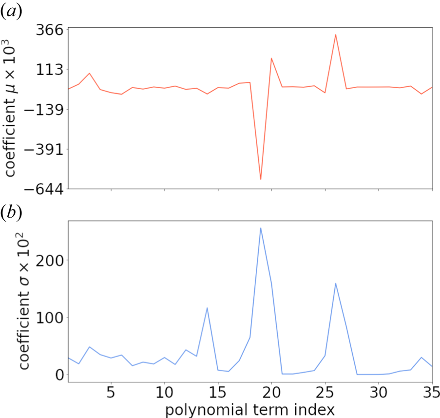
The mean and standard deviation versus polynomial term are shown in figure 9 excluding the constant term because it has a much larger mean value of $m_0 \approx 1.373\times 10^{-2}$ and standard deviation of $\sigma _0 \approx 7.314\times 10^{-3}$
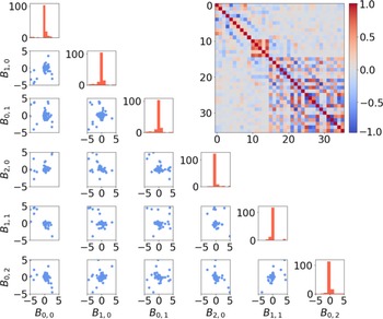
 . We can visualise the resulting distribution of coefficients using pair-wise scatter plots and histograms as in figure 10 which shows the coefficients for polynomials up to polynomial order two along with the covariance matrix for all orders up to $N_p^{\text {max}} = 8$
 . Figure 10 indicates that a zero-mean normal approximation $\tilde B_{n,m} \sim \mathcal {N}(0,\varLambda ^{n,m})$
 is reasonable as a prior on the background signal, where

is the covariance matrix of the (zero-mean) scaled background coefficients, where we have explicitly indicated the dependence of $n$ and $m$
 on $i$
 and $j$
 , that is, the choice of ordering for the polynomial terms specified earlier. We emphasise that this provides a useful prior distribution for adding background to any model in order to propagate the uncertainty due to the presence of background signal in applications such as that in Glinsky et al. (Reference Glinsky, Moore, Lewis, Weis, Jennings, Ampleford, Knapp, Harding, Gomez and Harvey-Thompson2020) and Knapp et al. (Reference Knapp, Glinsky, Schaeuble, Jennings, Evans, Gunning, Awe, Chandler, Geissel and Gomez2022). Alternately, it could be used as a prior in a Bayesian fit to the background signal for a given image, with the resulting posterior set of fit backgrounds providing a way to quantify uncertainty in the background subtraction process.
Coefficient (a) mean $m$ and (b) standard deviation $\sigma$
 values for the non-constant polynomial terms ordered as described in the text. The mean and standard deviation for the constant term are given by $m_{0} \approx 1.373\times 10^{-2}$
 and standard deviation of $\sigma _0 \approx 7.314\times 10^{-3}$
 .

The distribution of background coefficients for MagLIF stagnation images can be reasonably approximated by a multi-variate normal distribution as indicated by pair plots of the standard-normal scaled coefficient values up to second-order terms in the polynomial expansion of the background (blue points in scatter plots). The marginal distributions for each coefficient are of the corresponding coefficient labelled on the bottom are also shown on the diagonal, indicating a central peak along with a small number of outliers. The computed covariance matrix is shown as an inset in the upper-right corner.

3.2. Statistical analysis of noise
Now we highlight some important observations about the behaviour of noise statistics in our images. First, we note that minimising the loss given by (2.34) is equivalent to finding a maximum likelihood estimate (Bishop Reference Bishop2006) of the background coefficients with a Gaussian prior on the coefficients and assumed zero-mean and constant variance Gaussian statistics of the noise about the background signal. In other words, we assume that for each image, ${\rm BG}_\text {obs} = {\rm BG}_\text {model} + \epsilon$ , where $\epsilon$
 is distributed by a zero-mean normal distribution with standard deviation $\sigma _{\text {BG}}$
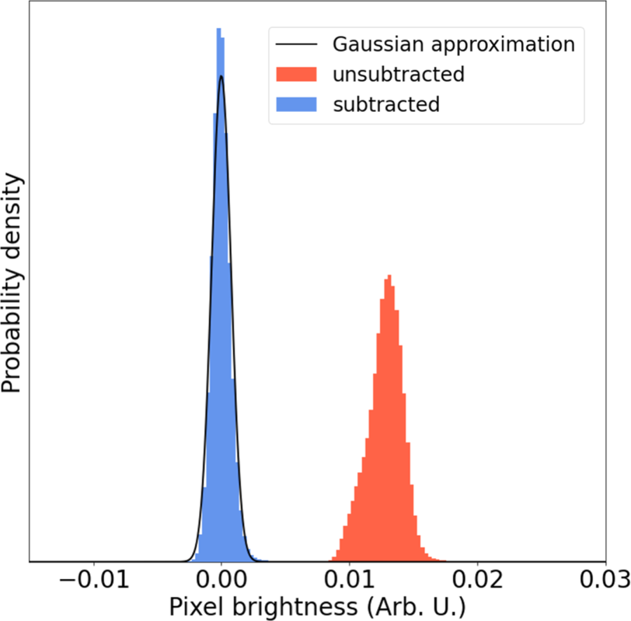
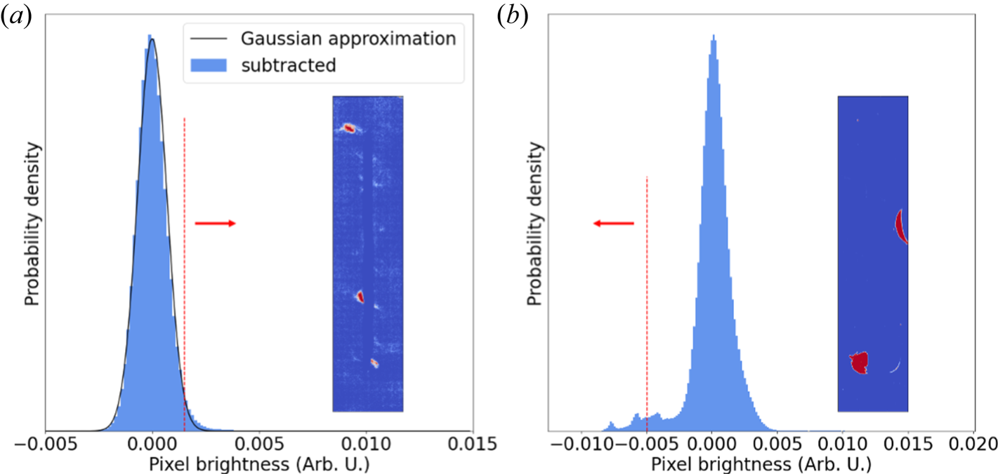
 that is allowed to be different for each image. Figure 11 shows an example of background-assigned pixel statistics before (red) and after (blue) subtracting the slowly varying background, we find that the residual noise is very well described by a zero-mean Gaussian distribution in this case. We note that any significant deviation from this distribution indicates either we have incorrectly assumed normally distributed noise or there is a failure of the polynomial background model to describe the observed signal variation. We consider the former unlikely, as the data collection process (recording of x-rays onto an image plate) and digitisation by plate scanning should be well described by a sum of poisson random variables with a high mean rate parameter so that the statistics are approximately Gaussian. Indeed, if we consider two cases showing significant deviation from a single zero-mean normal distribution for the pixel statistics after background subtraction, we see that significant statistics on the low side of the main peak are typically associated with image plate damage, whereas excess bright pixels are associated with extended emission structure from the target or other background signal that could not be effectively subtracted. We present two such cases in figure 12. For the first case shown on the left, there is a minor deviation from gaussian statistics in the high pixel brightness tail. The inset shows pixels with value greater than the $97.5{\text {th}}$
 percentile coloured red, indicating that these pixels are primarily associated with extended structure due to liner emission. In the second case, there is significant information in the low-brightness tail. Cutting at the $2.5{\text {th}}$
 percentile and colouring pixels whose value are less than this red, we see some regions of plate damage while pushing to even higher cuts would include even more plate damaged regions. We note however, that in general the cross-validation background fitting procedure appears to be effective in avoiding over-fitting to these types of background features.
Image noise appears to be well described in most cases with a normal distribution after the polynomial background subtraction is performed.

(a) The background pixels very nearly follow a normal distribution for most of our data. Slight discrepancies at the high-brightness tail are strongly correlated with emission from the cold liner and/or unsubtracted background signal. (b) One of a small number of cases where the background deviates significantly from a normal distribution. This occurs when there is plate damage, and the low-brightness pixels are strongly correlated with the regions of plate damage.

Another important quantity to constrain is the relative strength of the noise as compared with the strand signal, i.e. a SNR. There are multiple reasonable approaches to defining such a quantity. Here we choose to define the SNR as

where $\mathcal {S}_{95\,\%}$ is the $95\text {th}$
 percentile brightness value of pixels associated with the strand, and $\sigma _{\text {BG} }$
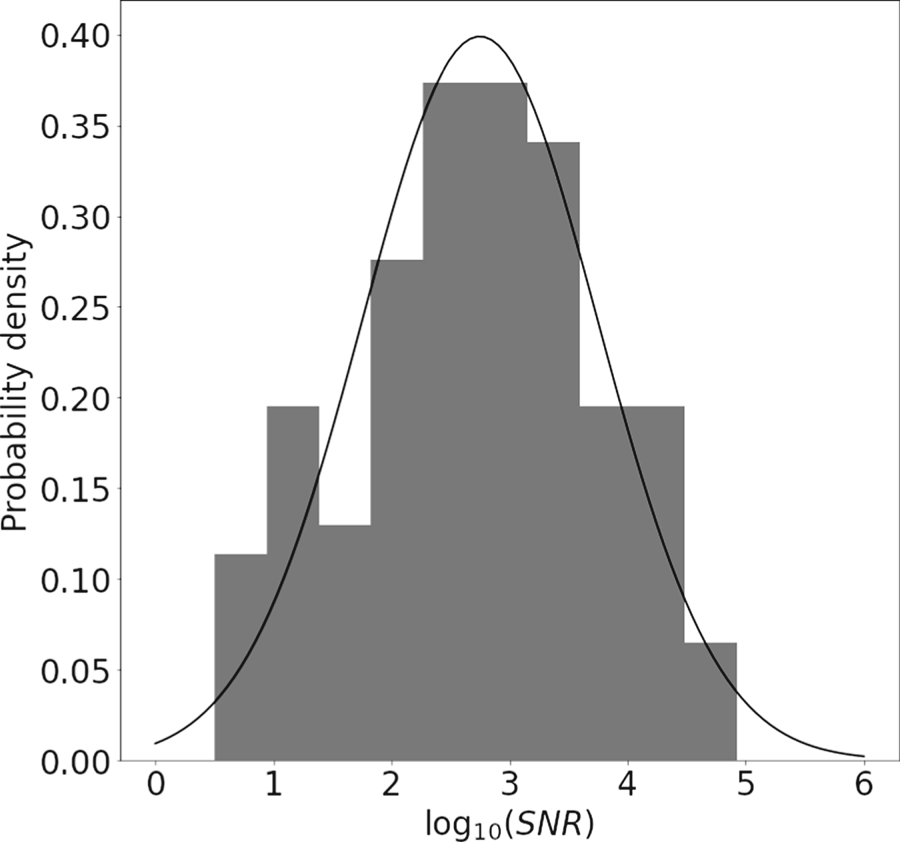
 is the standard deviation of the brightness value for pixels assigned to the background. In figure 13, we plot a histogram for $\log ({\rm SNR})$
 . Without higher statistics, it is difficult to accurately posit a prior distribution for the ${\rm SNR}$
 from experiment. However, it appears reasonable to approximate the distribution $\log ({\rm SNR}) \sim \mathcal {N}(2.75,1.0)$
 as shown in the black curve overlaying the experimental data distribution in figure 13.
Histogram showing the distribution of $\log ({\rm SNR})$ . Although the statistics are not sufficient to conclusively specify a detailed prior distribution for the SNR based on our data, a log-normal distribution as detailed in the text appears to provide reasonable agreement.

4. Conclusion and Future Work
We have demonstrated the use of a CNN to learn a segmentation map separating the fuel column from background in MagLIF stagnation images. Although the network was trained on data from a synthetic model which likely cannot capture all of the complexity in our experimental data, the relative simplicity of the segmentation task allowed the network to perform well without the need to apply transfer learning on our experimental dataset. In conjunction with a rules-based image registration pipeline, this enabled us to process data from $N_{\text {scans}} = 139$ SCXI image plate scans across $N_{\text {exp}} = 67$
 experiments.
By assessing the statistical properties of the background model fits and resulting noise distributions over our ensemble of images, we were able to provide prior distributions for background model parameters. These distributions will be useful in improving synthetic training datasets for machine learned models by include realistic background features. In addition, these priors can be used in Bayesian inferences using SCXI datasets to aid in quantifying uncertainty due to image processing stages, typically not incorporated in such analyses. We anticipate numerous additional extensions of this work going forward. In particular, we expect that we will be able to adapt this approach to multi-channel pinhole camera data (McPherson et al. Reference McPherson, Ampleford, Coverdale, Argo, Owen and Jaramillo2016; Knapp et al. Reference Knapp, Glinsky, Schaeuble, Jennings, Evans, Gunning, Awe, Chandler, Geissel and Gomez2022) in order to automatically extract electron temperature maps. In addition, the database created by our processing routine is used in a companion publication where we are able to assess sensitivities of an image metric based on a purely experimental-data-driven model-free basis (Lewis et al. unpublished observations). Finally, the pipeline demonstrated quickly produces labelled experimental datasets with relatively little user input. Pairing this labelled dataset with data-augmentation methods to handle rarely occurring artifacts in our images may enable training and validating fully automated end-to-end pipelines without reference to a synthetic model as more experimental data become available.
Acknowledgements
W.E. Lewis would like to thank R. Patel for useful feedback along with G. Dunham for useful discussions regarding image plate data digitisation. This article has been authored by an employee of National Technology & Engineering Solutions of Sandia, LLC under Contract No. DE-NA0003525 with the U.S. Department of Energy (DOE). The employee owns all right, title and interest in and to the article and is solely responsible for its contents. The United States Government retains and the publisher, by accepting the article for publication, acknowledges that the United States Government retains a non-exclusive, paid-up, irrevocable, world-wide license to publish or reproduce the published form of this article or allow others to do so, for United States Government purposes. The DOE will provide public access to these results of federally sponsored research in accordance with the DOE Public Access Plan https://www.energy.gov/downloads/doe-public-access-plan.
Editor William Dorland thanks the referees for their advice in evaluating this article.
Declaration of interests
The authors report no conflict of interest.