Structure of the streaming flow generated by a sphere in a fluid undergoing rectilinear oscillation

Peijing Li; Jesse F. Collis; Douglas R. Brumley; Lennart Schneiders; John E. Sader

doi:10.1017/jfm.2023.758

Structure of the streaming flow generated by a sphere in a fluid undergoing rectilinear oscillation

Published online by Cambridge University Press: 03 November 2023

and

Peijing Li: Affiliation:
School of Mathematics and Statistics, The University of Melbourne, Victoria 3010, Australia
Jesse F. Collis: Affiliation:
School of Mathematics and Statistics, The University of Melbourne, Victoria 3010, Australia
Douglas R. Brumley: Affiliation:
School of Mathematics and Statistics, The University of Melbourne, Victoria 3010, Australia
Lennart Schneiders: Affiliation:
Division of Engineering and Applied Science, California Institute of Technology, Pasadena, CA 91125, USA
John E. Sader*: Affiliation:
Graduate Aerospace Laboratories and Department of Applied Physics, California Institute of Technology, Pasadena, CA 91125, USA
*: †Email address for correspondence: jsader@caltech.edu

Article contents

Abstract
Introduction
Small-amplitude flows
Finite-amplitude flows
Conclusions
Funding
Declaration of interests
References

Rights & Permissions

Abstract

A solid body in a viscous fluid undergoing oscillatory motion naturally produces a steady secondary flow due to convective inertia. This phenomenon is embodied in the streaming flow generated by a sphere in an unbounded fluid executing rectilinear oscillations. We review the considerable literature on this canonical problem and summarise exact and asymptotic formulas in the small-amplitude limit. These analytical formulas are used to explore the characteristic flow structure of this problem and clarify previously unreported features. A single, toroidal-shaped vortex exists in each hemisphere regardless of the oscillation frequency, which can drive a counter-flow away from the sphere. The vortex centre moves monotonically away from the sphere with decreasing oscillation frequency, and engulfs the entire flow domain for $\beta \equiv \omega R^2/\nu < 16.317$, where $\omega$ is the angular oscillation frequency, $R$ the sphere radius, and $\nu$ the fluid kinematic viscosity. This seemingly abrupt change in flow structure at the critical frequency $\beta _{critical} =16.317$, and its quantification, appear to have not been reported previously. We perform a direct numerical simulation of the Navier–Stokes equations, to (1) confirm existence of this critical frequency at finite amplitude, and (2) examine its variation with amplitude. This reveals a universal relationship between the critical frequency and oscillation amplitude, clarifying previous reports on the structure of this streaming flow. The critical frequency is shown to be identical for the streaming flow and the cycle-averaged particle paths, establishing that the critical frequency is accessible directly using standard measurements.

JFM classification

Micro-/Nano-fluid dynamics: Microscale transport Mathematical Foundations: General fluid mechanics

Information

Type: JFM Papers
Information: Journal of Fluid Mechanics , Volume 974 , 10 November 2023, A37
DOI: https://doi.org/10.1017/jfm.2023.758 [Opens in a new window]
Copyright: © The Author(s), 2023. Published by Cambridge University Press

1. Introduction

The oscillatory motion of solid bodies in viscous fluids has been studied widely since the time of Stokes, who explored how such fluids affect the motion of pendulums (Stokes Reference Stokes1851). By assuming a small oscillation amplitude, Stokes ignored the effects of convective inertia and linearised the equations of motion. This greatly simplified the analysis, which enabled analytical solutions to be developed. Stokes (Reference Stokes1851) reported formulas for several canonical flow problems, including the inertialess drag on a sphere and the unsteady force experienced by a sphere executing small rectilinear oscillations, that now form the foundations for a multitude of applications.

It is recognised widely that oscillatory motion of a solid body can generate a steady flow due to nonlinear effects. This ‘acoustic streaming’ phenomenon was first explained theoretically by Rayleigh (Reference Rayleigh1884). In his analysis of the circulation of air in Kundt's tubes, Lord Rayleigh showed that a confluence of (nonlinear) convective inertia and viscosity near a solid boundary is required to drive the steady circulatory flow. By continuity, this near surface flow generates a counter-flow away from the surface. This double flow structure has since been examined under different flow conditions and geometries, and is a characteristic feature of streaming flows (Riley Reference Riley2001).

The oscillatory motion of a sphere in a viscous fluid is a canonical problem that has received considerable attention. Its steady streaming flow was first studied theoretically by Lane (Reference Lane1955), who analysed small-amplitude oscillations at small Reynolds number and derived an analytical solution for arbitrary oscillation frequency. This theory was compared to measurements on spheres, where significant differences were noted, in contrast to the good agreement found previously for cylinders (Raney, Corelli & Westervelt Reference Raney, Corelli and Westervelt1954). A decade later, Riley (Reference Riley1966) reported a landmark study on the small-amplitude oscillatory flow about a sphere, where an asymptotic analysis of its streaming flow was provided in the small- and large-frequency limits. Riley (Reference Riley1966) showed that the above-mentioned counter-flow structure is present around a sphere at large frequency, but vanishes in the small-frequency limit where the near-surface circulatory cell occupies the entire flow domain; intermediate finite frequencies were not studied. Increasing the oscillation frequency in the large-frequency limit decreases the thickness of the near-surface circulatory cell – consistent with a decrease in the viscous penetration depth of the linear oscillatory flow driving the streaming flow. However, these circulatory cells near the surface do not appear around soft bubbles. Later works, for example by Davidson & Riley (Reference Davidson and Riley1971), Wu & Du (Reference Wu and Du1997) and Longuet-Higgins (Reference Longuet-Higgins1998), study the flow around a bubble performing small-amplitude oscillations. The streaming flow at large frequency was observed to consist of only one region with velocity vectors in the opposite direction to the outer flow of a solid sphere. There is no (inner) circulation cell near the bubble surface at large frequency (Davidson & Riley Reference Davidson and Riley1971). More recently, Dōhara (Reference Dhara1982) reported an alternative analytical solution for the small-amplitude streaming flow generated by a sphere at arbitrary frequency, with the aim of obtaining ‘more exact results for the steady streaming than Lane and Riley's’. The relative merits of the complementary analytical solutions of Lane (Reference Lane1955) and Dōhara (Reference Dhara1982) were not reported at the time, which we now clarify.

The theory of Lane (Reference Lane1955) for a sphere is based on an extension of that author's analytical solution for a cylinder (Raney et al. Reference Raney, Corelli and Westervelt1954). However, Lane (Reference Lane1955) makes an error that invalidates the analysis, by choosing

(1.1)

\begin{equation} \left[(\boldsymbol{\nabla} \times \boldsymbol{u}) \boldsymbol{\cdot} \boldsymbol{\nabla}\right]\boldsymbol{u}=\boldsymbol{0}, \end{equation}

where $\boldsymbol {u}$ is the velocity field. While (1.1) holds for the two-dimensional flow generated by a cylinder (the origin of this identity), the same is not true for the axisymmetric flow about a sphere, i.e. $[(\boldsymbol {\nabla } \times \boldsymbol {u}) \boldsymbol {\cdot } \boldsymbol {\nabla }]\boldsymbol {u} \neq \boldsymbol {0}$. Specifically, while the vorticity lies in the azimuthal direction, the directional derivative of the velocity in this direction is not zero because the basis vectors in the radial and polar directions depend on the azimuthal coordinate. It appears this error is responsible for the disagreement observed between theory and measurements (Lane Reference Lane1955), mentioned above. The theory of Dōhara (Reference Dhara1982) does not employ the erroneous vector identity in (1.1). However, the analytical solution of Dōhara (Reference Dhara1982) is yet to be validated against asymptotic solutions (e.g. Wang Reference Wang1965; Riley Reference Riley1966) or independent numerical results, and its validity remains unconfirmed.

Asymptotic analysis has been reported on the streaming flow in the large (convective) Reynolds number limit, at small oscillation amplitude. Wang (Reference Wang1965) performed an asymptotic analysis on the boundary layer equations for such an oscillatory flow past a sphere. The resulting streaming flow exhibits a qualitatively similar structure to the large-frequency limit at small convective Reynolds number. Stuart (Reference Stuart1966) studied the small-amplitude oscillatory flow past a two-dimensional cylinder, and identified the following condition for existence of a ‘double boundary layer’ in the streaming flow:

(1.2)

\begin{equation} {\textit{Re}}_s \equiv \frac{U^2}{\omega \nu} \gg 1, \end{equation}

where $U$ is a characteristic flow speed of the oscillatory flow, $\omega$ is the angular oscillation frequency, and $\nu$ is the fluid kinematic viscosity. More specifically, the thicknesses of both inner and outer boundary layers are small compared to the cylinder radius.

Considerable effort has also focused on computing numerically the streaming flows generated by oscillating spheres. Chang & Maxey (Reference Chang and Maxey1994) performed direct numerical simulations (DNS) of the Navier–Stokes equations and determined the streaming flow generated by an oscillating sphere in quiescent fluid under a wide range of conditions. This was not restricted to the small-amplitude limit discussed above. By the nature of their numerical approach, Chang & Maxey (Reference Chang and Maxey1994) were able to study amplitudes that greatly exceed the sphere radius. The above-mentioned counter-flow structure of the streaming flow was not always observed. This was compared to the condition of Stuart (Reference Stuart1966) in (1.2), which was observed not to apply to larger amplitude oscillations. Chang & Maxey (Reference Chang and Maxey1994) comment: ‘There do not appear to be any generalisations that can be made for the existence of inner and outer streaming regions for flows of all amplitudes.’ Here, we explore the structure of the streaming flow and provide the generalisation sought by Chang & Maxey (Reference Chang and Maxey1994).

Mei (Reference Mei1994) also analysed both the steady and unsteady flow around a sphere using DNS. In the large-frequency and small-amplitude limit, their simulations showed good agreement with the asymptotic solution of Riley (Reference Riley1966), while discrepancy grew with increasing amplitude. Flows at large frequency contained two cells; see figure 6 of Mei (Reference Mei1994). In the small-frequency and large-amplitude limit, $\epsilon ^{-1} \ll {\textit {Re}} \ll 1$, where $\epsilon$ is the dimensionless Lagrangian amplitude defined by

(1.3)

\begin{equation} \epsilon \equiv \frac{U}{\omega R}, \end{equation}

and the (convective) Reynolds number is ${\textit {Re}}\equiv \epsilon \beta$, where

(1.4)

\begin{equation} \beta \equiv \frac{\omega R^2}{\nu}, \end{equation}

and $R$ is the sphere radius. Mei (Reference Mei1994) identified several length scales (non-dimensionalised by the sphere radius) for the unsteady flow field: (1) $r = O(1)$ for the inner region near the sphere; (2) $r= O({\textit {Re}}^{-1})$ and $r= O(\beta ^{-{1}/{2}})$ for the intermediate region away from the sphere; and (3) $r= O(\epsilon )$ for the transverse and streamwise flow direction far from the sphere. However, there was no discussion pertaining to how the flow structure relates to these length scales.

The (incompressible) streaming flow is fully characterised by two independent dimensionless groups (Blackburn Reference Blackburn2002), which we choose here to be the dimensionless frequency $\beta$ and the Lagrangian oscillation amplitude $\epsilon$. All other dimensionless parameters reported in the literature are derivatives of these two groups, including (1.2). This relationship between the dimensionless groups, together with the observation in (1.4), suggests a universality in the counter-flow structure – contrary to the assertion of Chang & Maxey (Reference Chang and Maxey1994) mentioned above – which we explore in this study.

Blackburn (Reference Blackburn2002) also conducted a DNS study and reported that in the Stokes limit, i.e. at zero frequency, only the inner circulation cell remains – consistent with the asymptotic analysis of Riley (Reference Riley1966). Alassar (Reference Alassar2008) studied the streaming flow for moderate to large dimensionless frequency, at finite oscillation amplitude, finding that the inner circulatory cell thickness grows with decreasing oscillatory frequency. An empirical fit formula based on their DNS numerical data indicates that this thickness varies as a fractional power of the reciprocal frequency. While this suggests that the inner circulatory flow engulfs the flow domain in the zero frequency limit only, this conclusion is based on simulations away from the small-frequency limit. Chan et al. (Reference Chan, Bhosale, Parthasarathy and Gazzola2022) have also performed numerical simulations at small amplitude, and find that the counter-flow structure is present only at larger frequencies, with smaller frequencies exhibiting a single circulation cell. Indeed, a recent DNS study by Fabre et al. (Reference Fabre, Jalal, Leontini and Manasseh2017) found that at a small but finite frequency, the streaming flow around a pair of spheres does not exhibit a counter-flow structure. This finding is consistent with theoretical studies of other geometries (Kaneko & Honji Reference Kaneko and Honji1979; Carlsson, Sen & Löfdahl Reference Carlsson, Sen and Löfdahl2004; Bhosale et al. Reference Bhosale, Vishwanathan, Upadhyay, Parthasarathy, Juarez and Gazzola2022) that show that the characteristic counter-flow structure of streaming flows exists only above a distinct non-zero frequency and is geometry dependent.

Experiments have been conducted to explore the counter-flow structure of streaming flows. Lutz, Chen & Schwartz (Reference Lutz, Chen and Schwartz2005) compared their measurements for a cylinder to the theory of Bertelsen, Svardal & Tjøtta (Reference Bertelsen, Svardal and Tjøtta1973). Figure 5 of Lutz et al. (Reference Lutz, Chen and Schwartz2005) indicates that the size of the inner circulation cell diverges at finite frequency. That is, the above-mentioned transition in flow structure occurs for both cylinders and spheres, and has been observed experimentally for a cylinder. The relationship predicted theoretically by Bertelsen et al. (Reference Bertelsen, Svardal and Tjøtta1973), between the thickness of the (steady) inner circulatory cell and that of the (oscillatory) viscous penetration depth, was validated experimentally for a range of cylinders; the former thickness always exceeds the latter. In a series of subsequent studies, Kotas, Yoda & Rogers (Reference Kotas, Yoda and Rogers2006, Reference Kotas, Yoda and Rogers2007, Reference Kotas, Yoda and Rogers2008) reported measurements of the streaming flows generated by spheroids. They found that the thickness of the inner region varies with the reciprocal of the frequency, for which similar behaviour was noted in the computational study of Alassar (Reference Alassar2008) discussed above. This scaling law for the inner region thickness was verified experimentally by Otto, Riegler & Voth (Reference Otto, Riegler and Voth2008). However, these experimental studies again did not systematically investigate the small-frequency limit, and their resulting empirical relations, based on experimental data, should be considered large-frequency scaling laws only.

The aim of this study is to address the above-mentioned outstanding issues for streaming flows around a sphere using a combination of analytical and numerical solutions. Specifically, we validate the analytical solution of Dōhara (Reference Dhara1982) against independent analytical solutions in the small-amplitude limit. These include analytical solutions for small and large frequency, and a new analytical solution for arbitrary frequency. We show that, in this small-amplitude limit, the streaming flow exhibits the usual characteristics found around other solid bodies: a counter-flow structure at large frequency, while the inner vortex cell engulfs the entire flow domain below a distinct non-zero frequency

(1.5)

\begin{equation} \beta_{critical} = 16.317\ldots, \end{equation}

a result that does not appear to have been reported previously. The applicability of this result to streaming flows at finite amplitude is then explored using new DNS solutions of the Navier–Stokes equations, from which a universal relationship between $\beta _{critical}$ and the oscillation amplitude $\epsilon$ is revealed. While our primary motivation is to unify the numerous numerical studies on this problem, the intermediate to large amplitude regime is relevant to biological/artificial swimmers, and may provide insight into the flow structure around swimmers whose stroke motion is at moderate Reynolds number (Gemmell, Jiang & Buskey Reference Gemmell, Jiang and Buskey2015; Mohaghar, Adhikari & Webster Reference Mohaghar, Adhikari and Webster2019; Dombrowski & Klotsa Reference Dombrowski and Klotsa2020). It may also find application to cylindrical and spherical bodies in unsteady flows relevant to oceanographic research, where the flow remains laminar before the onset of instabilities (Sarpkaya & Storm Reference Sarpkaya and Storm1985; Wybrow, Yan & Riley Reference Wybrow, Yan and Riley1996; Ren et al. Reference Ren, Cheng, Tong, Xiong and Chen2019).

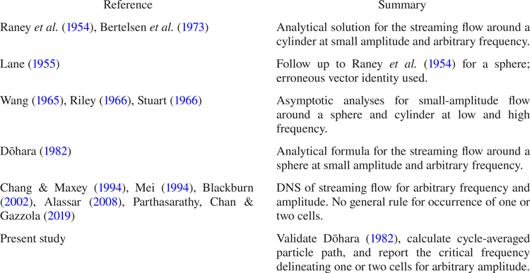
A comparison is also made between the streaming flow and cycle-averaged particle paths – termed the ‘particle motion’ – which is relevant to experimental measurements of the streaming flow. Differences are observed, particularly at small frequency and small amplitude. Even so, the critical frequency is found to be identical for the streaming flow and particle motion. This guides potential future efforts to measure this frequency experimentally. Table 1 places the present work in the context of previous studies of this streaming flow.

Table 1.

Theoretical studies of the steady streaming flow generated by an oscillating sphere/cylinder.

2. Small-amplitude flows

We first study the limiting case of small oscillation amplitude. Analytical formulas are presented for the streaming flow and particle motion at small, large and arbitrary frequency. This complements existing literature formulas (Wang Reference Wang1965; Riley Reference Riley1966; Dōhara Reference Dhara1982), as discussed in § 1.

2.1. Analytical solution

Consider a stationary sphere in an incompressible, unbounded fluid that far from the sphere is executing small-amplitude oscillations with velocity $\mathrm {Re}[U\,\mathrm {e}^{-\text {i}\omega t} \boldsymbol {k}]$, where $\mathrm {Re}$ denotes the real part of the expression, $U$ is the maximum speed, $\boldsymbol {k}$ is the Cartesian basis vector in the $z$-direction, $\text {i}$ is the imaginary unit, and $t$ is time. The streaming flow generated by an oscillating sphere in a quiescent fluid follows directly, if needed (Westervelt Reference Westervelt1953a). The dimensionless governing equation is

(2.1)

\begin{equation} \beta \left( \frac{\partial }{\partial t}+\epsilon L^2_{\varPsi} \right) D^2 \varPsi = D^4 \varPsi, \end{equation}

with $\varPsi$ being the Stokes stream function,

(2.2a)

$$\begin{gather} D^2 \equiv \frac{\partial^2 }{\partial r^2}+\frac{\sin{\theta}}{r^2}\,\frac{\partial }{\partial \theta} \left( \frac{1}{\sin \theta}\,\frac{\partial }{\partial \theta} \right) , \end{gather}$$

(2.2b)

$$\begin{gather}L^2_{\varPsi} \equiv \frac{1}{r^2\sin{\theta}} \left(\frac{\partial \varPsi}{\partial \theta}\,\frac{\partial }{\partial r}-\frac{\partial \varPsi}{\partial r}\,\frac{\partial }{\partial \theta}+2\cot{\theta} \, \frac{\partial \varPsi}{\partial r}-\frac{2}{r}\,\frac{\partial \varPsi}{\partial \theta}\right), \end{gather}$$

where $D^4 = D^2 D^2$, and $r$ and $\theta$ are the radial and polar angle spherical coordinates, respectively, whose origin is at the sphere centre. The radial coordinate is scaled by the sphere radius $R$, the stream function by $U R^2$, and time by $1/\omega$. The dimensionless oscillation amplitude $\epsilon$, and dimensionless frequency $\beta$, are respectively defined in (1.3) and (1.4). The corresponding boundary conditions of no-slip at the particle surface and uniform oscillation of the far field lead to

(2.3)

\begin{equation} \left.\frac{\partial \varPsi}{\partial \theta} \right|_{r=1} = \left. \frac{\partial \varPsi}{\partial r} \right|_{r=1} =0, \quad \varPsi |_{r\to\infty} \sim \mathrm{Re}\left[\frac{r^2}{2}\sin^2\theta \, \mathrm{e}^{-\text{i}t}\right], \end{equation}

and we choose $\varPsi =0$ at $r=1$ in line with previous literature.

Equations (2.1) and (2.3) are to be solved in the small-amplitude asymptotic limit, $\epsilon \rightarrow 0$, for which we accordingly expand the stream function as

(2.4)

\begin{equation} \varPsi=\varPsi^{(0)}+\epsilon \varPsi^{(1)}+o(\epsilon). \end{equation}

Substituting (2.4) into (2.1) and (2.3) gives the respective governing equations and boundary conditions for $\varPsi ^{(0)}$ and $\varPsi ^{(1)}$. In Fourier space, the leading-order governing equation becomes

(2.5)

\begin{equation} D^2 ( D^2 + \text{i} \beta ) \psi^{(0)} = 0, \end{equation}

where $\varPsi ^{(0)}(r,\theta,t)=\mathrm {Re}[{\psi ^{(0)}(r,\theta )\, \mathrm {e}^{-\text {i} t}]}$. The governing equation at $O(\epsilon )$ produces a flow $\varPsi ^{(1)}$ with (i) a periodic component at twice the frequency of the boundary condition in (2.3), and (ii) a steady component $\psi ^{(1)}$, which is the required streaming flow. The governing equation for the latter is

(2.6)

\begin{equation} D^4 \psi^{(1)} = \frac{ \beta}{4} ( L^2_{\psi^{(0)}} D^2 \psi^{(0)*} + L^2_{\psi^{(0)*}} D^2 \psi^{(0)}), \end{equation}

with the starred quantities referring to their complex conjugates.

Because the asymptotic expansion in (2.4) is with respect to $\epsilon$ only, $\beta$ is implicitly finite. Consequently, (2.4) gives the solution in the small Reynolds number limit,

(2.7)

\begin{equation} {\textit{Re}} \equiv \epsilon \beta \rightarrow 0, \end{equation}

establishing that

(2.8)

\begin{equation} {\textit{Re}}_s \equiv \epsilon\,{\textit{Re}} \rightarrow 0. \end{equation}

That is, the steady streaming Reynolds number in (1.2) vanishes, and a double boundary layer in the streaming flow does not exist. The solution for $\psi ^{(0)}$ is well known (Stokes Reference Stokes1851),

(2.9)

\begin{align} \psi^{(0)} = \left(\frac{r^2}{2}-\frac{3}{2 r}\left[\frac{1}{3}+\frac{3\text{i}}{\beta}+\frac{1+\text{i}}{\sqrt{2\beta}}\right]+\frac{3}{2} \,{\rm e}^{-\sqrt{{\beta}/{2}}\,(1-\text{i}) (r-1)} \left[\frac{1+\text{i}}{\sqrt{2\beta}}+\frac{\text{i}}{\beta r}\right]\right) \sin^2\theta,\end{align}

while we calculate the solution for $\psi ^{(1)}$ to be

(2.10)

\begin{align} \psi^{(1)}&= \left\{\,f_{1} + \frac{f_{2}}{r^2} + f_{3}(r)\,E_{1} (\sqrt{2 \beta}\, r)+f_{4}(r)\,E_{1} \left((1+\mathrm{i})\,\sqrt{\frac{\beta}{2}}\,r\right)\right.\nonumber\\ &\quad+f_{4}^{*}(r)\,E_{1} \left((1-\mathrm{i})\,\sqrt{\frac{\beta}{2}}\,r\right) + f_{5}(r)\,\mathrm{e}^{-\sqrt{2 \beta}\,(r-1)}\nonumber\\ &\left.\quad{}+f_{6}(r)\,{\rm e}^{-(1+\mathrm{i})\sqrt{{\beta}/{2}}\,(r-1)}+f_{6}^{*}(r)\, {\rm e}^{-(1-\mathrm{i})\sqrt{{\beta}/{2}}\,(r-1)}\vphantom{\left((1+\mathrm{i})\sqrt{\frac{\beta}{2}} r\right)}\right\} \cos\theta \sin^2\theta, \end{align}

where the constants $f_{1},\, f_{2}$, together with radial functions $f_{3}(r)$, $f_{4}(r)$, $f_{5}(r)$, $f_{6}(r)$, are defined explicitly in Appendix A, and $E_{1}(z) \equiv \int _{1}^{\infty } \tau ^{-1}\,\mathrm {e}^{- z \tau }\,\text {d}\tau$ is the exponential integral function. Due to the lengthy nature of the $f_i$ terms, supplementary material is provided (available at https://doi.org/10.1017/jfm.2023.758) that implements (2.10).

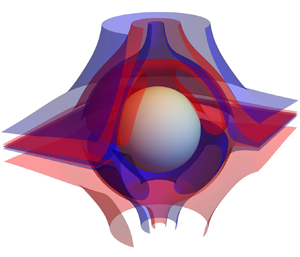
Figure 1 shows the true flow structure of the steady-streaming flow, illustrated by the level sets of (2.10), i.e. the streamtubes. Figure 1(a) shows the streaming flow at low $\beta$, where a single toroidal vortex encompasses the entire domain in each hemisphere, henceforth referred to as the ‘one-cell’ structure. Figure 1(b) shows the streaming flow at high $\beta$, where an inner toroidal vortex occurs in each hemisphere. The outer region contains open sheets that extend to infinity and do not close. This inner/outer structure is termed the ‘two-cell’ structure.

Figure 1.

Three-dimensional level sets of the stream function for the streaming flow: (a) $\beta = 0.1$, (b) $\beta = 20$. The asymptotic formulas in (2.14) and (2.19) for small and large frequency are used. Blue and red surfaces are used to guide the eye, and the sphere is shaded in grey. The black double arrow gives the direction of the oscillating far-field velocity.

2.1.1. Relationship to analytical formula of Dōhara (Reference Dhara1982)

Comparison of (2.10) to equation (17) of Dōhara (Reference Dhara1982) shows that while they differ superficially – being expressed in terms of complex and real functions, respectively – these complementary formulas for the streaming flow are mathematically equivalent; see the Mathematica notebook in the supplementary material.

The primary difference in their application is that equation (17) of Dōhara (Reference Dhara1982) requires evaluation of an indefinite integral of non-standard form, while (2.10) is expressed in terms of standard mathematical functions. This comparison provides independent validation of the theory of Dōhara (Reference Dhara1982), which is yet to be reported.

2.2. Cycle-averaged particle paths

Because the streaming flow is the steady component of a more general oscillatory flow, it is often measured experimentally by tracking the long-time motion of small particles placed in the flow, i.e. the cycle-averaged particle paths. This particle motion naturally includes the effect of Stokes drift (Longuet-Higgins Reference Longuet-Higgins1953), which is absent from (2.10). The required stream function defining the overall particle velocity averaged over one oscillation cycle is (Longuet-Higgins Reference Longuet-Higgins1953)

(2.11)

\begin{equation} \psi_{particle}^{(1)} =\psi^{(1)}+\psi_D . \end{equation}

Following Westervelt (Reference Westervelt1953b), the Stokes drift contribution is

(2.12)

\begin{equation} \psi_D =\frac{ -\text{i}}{4 r^2\sin{\theta}}\left( \frac{\partial \psi^{(0)*}}{\partial \theta}\,\frac{\partial \psi^{(0)}}{\partial r}- \frac{\partial \psi^{(0)*}}{\partial r}\,\frac{\partial \psi^{(0)}}{\partial \theta}\right){,} \end{equation}

whose explicit formula is given in Appendix A. Westervelt (Reference Westervelt1953a) showed that the cycle-averaged particle motion generated by a stationary sphere in an oscillating fluid (the present case) is identical to that generated by a sphere oscillating in an otherwise quiescent fluid. Consequently, (2.11) and (2.12) apply to both situations.

2.3. Asymptotic solutions for small and large frequency $\beta$

To validate the analytical solution in (2.10), and (2.11) for the cycle-averaged particle motion, we derive independently asymptotic solutions in the limits of small and large $\beta$. This is achieved by performing a matched asymptotic expansion of (2.5) and (2.6), the details of which are given in Appendix B for completeness. These formulas complement previous asymptotic analyses by Wang (Reference Wang1965) and Riley (Reference Riley1966), who provided alternative analyses for large frequency and did not report the cycle-averaged particle paths.

Importantly, Taylor expansions of (2.10) and (2.11) for small and large $\beta$ are found to give formulas identical to the asymptotic results in Appendix B; see the Mathematica notebook in the supplementary material. This provides independent validation of (2.10) and (2.11). The resulting asymptotic formulas are summarised below for convenience.

2.3.1. Small oscillation frequency, $\beta \ll 1$

The inner region for the matched asymptotic expansion in small $\beta$ is $r \ll \beta ^{-{1}/{2}}$, with $r \gg \beta ^{-{1}/{2}}$ being the outer region.

The asymptotic solution for the steady streaming flow in the inner region is (Riley Reference Riley1966)

(2.13)

\begin{equation} \psi^{(1)} =\beta \left(-\frac{3 r^2}{32}-\frac{3}{64 r^2}+\frac{9 r}{64}+\frac{3}{64 r}-\frac{3}{64}\right)\cos\theta\sin^2\theta + o(\beta) , \end{equation}

while for the outer region,

(2.14)

\begin{align} \bar{\psi}^{(1)} = \frac{9 \beta}{16} \left( \mathrm{e}^{-\rho} \left[ \left( \frac{2}{3} +\frac{1}{\rho} \right) \sin \rho + \left(\frac{1}{\rho} +\frac{1}{\rho^2}\right) \cos \rho\right] - \frac{1}{\rho^2} \right)\cos{\theta}\sin^2\theta + o(\beta) , \end{align}

where $\rho =\sqrt {\beta /2}\,r$ and $\bar {\psi }^{(1)} = (\beta /2) \,\psi ^{(1)}$.

The corresponding formulas for the stream function defining the cycle-averaged particle motion in the inner region is

(2.15)

\begin{equation} \psi_{particle}^{(1)} =-\frac{3 \beta}{64} \left(3 r+3-\frac{2}{r}\right) \left(1-\frac{1}{r}\right)^2 \cos\theta\sin^2\theta + o(\beta), \end{equation}

and for the outer region,

(2.16)

\begin{equation} \bar{\psi}^{(1)}_{particle} = o(\beta) {,} \end{equation}

because the Stokes drift velocity at the outer region is

(2.17)

\begin{align} \bar{\psi}_{D} =-\frac{9 \beta}{16} \left( \mathrm{e}^{-\rho} \left[ \left( \frac{2}{3} +\frac{1}{\rho} \right) \sin \rho + \left(\frac{1}{\rho} +\frac{1}{\rho^2}\right) \cos \rho\right] - \frac{1}{\rho^2} \right)\cos{\theta}\sin^2\theta + o(\beta) , \end{align}

which exactly cancels out the streaming flow in the outer region at $O(\beta )$.

2.3.2. Large oscillation frequency, $\beta \gg 1$

The inner and outer regions for the matched asymptotic expansion in large $\beta$ are $r -1 \ll \beta ^{-{1}/{2}}$ and $r -1 \gg \beta ^{-{1}/{2}}$, respectively.

The asymptotic solution for the steady streaming flow in the outer region is (Riley Reference Riley1966)

(2.18)

\begin{equation} \psi^{(1)} = \frac{45}{32}\left(1-\frac{1}{r^2}\right) \cos{\theta}\sin^2 \theta +o(1), \end{equation}

and for the inner region,

(2.19)

$$\begin{align} \bar{\psi}^{(1)} &= \left(-\frac{189}{32}+\frac{45}{16}\,\eta+ \frac{9}{32} \left[\mathrm{e}^{-2\eta}+20 \mathrm{e}^{-\eta}\cos{\eta}+4\mathrm{e}^{-\eta}(3+2\eta)\sin{\eta}\right]\right) \nonumber\\ &\quad \,\times \cos{\theta}\sin^2 \theta + o(1) , \end{align}$$

where $\eta = \sqrt {\beta /2}\, (r-1)$ and $\bar {\psi }^{(1)} = \sqrt {\beta /2} \, \psi ^{(1)}$.

The corresponding formula for the stream function defining the cycle-averaged particle motion in the outer region is

(2.20)

\begin{equation} \psi_{particle}^{(1)} = \frac{45}{32}\left(1-\frac{1}{r^2}\right) \cos{\theta}\sin^2 \theta +o(1), \end{equation}

because the Stokes drift provides no contribution in the outer region at $O(\beta ^{-1})$, while for the inner region,

(2.21)

\begin{equation} \bar{\psi}_{particle}^{(1)} = \frac{9}{32} \left(10\eta-17 +12 \mathrm{e}^{-\eta}[\cos{\eta}+\sin{\eta}] + 5 \mathrm{e}^{-2\eta} \right) \cos{\theta}\sin^2 \theta + o(1) . \end{equation}

2.4. Results and discussion

We now examine the properties of the streaming flow and cycle-averaged particle motion, using the above-mentioned formulas.

2.4.1. Implications of asymptotic formulas for small and large $\beta$

The simple mathematical forms of the asymptotic formulas for small and large $\beta$ provide insight into the underlying structures of the streaming flow and the particle motion.

For small $\beta$, the leading-order streaming flow in (2.13) and (2.14) contains periodic functions in the radial coordinate, for the outer region only, i.e. $r \gg \beta ^{-{1}/{2}}$. This indicates that a vortex structure exists in the outer region only, which is highlighted in figures 2(c,d) for $\beta = 0.001$; note that the vortex centre occurs at $r = O(\beta ^{-{1}/{2}})$. In contrast, the asymptotic analysis shows that the cycle-averaged particle motion in the outer region is zero at $O(\beta )$. We note, however, that cycle-averaged particle motion does occur in the outer region at higher order, which is captured in the arbitrary-$\beta$ analysis. Moreover, periodic functions in the radial coordinate do not exist in (2.15), suggesting that particle motion may not orbit a centre in the inner region at leading order ($O(\beta )$). The particle motion using the exact solution is explored in § 2.4.2.

Figure 2.

Streamlines in the asymptotic limit of small $\beta$, to $O(\beta )$, of (a,b) inner and (c,d) outer regions of the streaming flow, using (2.13) and (2.14), respectively, for (a,c), and the cycle-averaged particle motion using (2.15) and (2.16), respectively, for (b,d). Cycle-averaged particle motion in the outer region is zero to $O(\beta )$; however, there is motion at higher order in $\beta$. The double arrow gives the direction of flow far from the stationary sphere. Red streamlines are to guide the eye.

For large $\beta$, we observe that periodic functions in the radial coordinate appear only in (2.19), indicating that a vortex occurs only in the inner region. Figure 3 shows this behaviour for $\beta =500$. In contrast to the small $\beta$ formulas of § 2.3.1, periodic functions in the radial coordinate persist in the presence of Stokes drift. These periodic functions occur only in the inner region; see (2.21). We therefore conclude that particles in the outer region do not orbit a centre, which is evident in the example in figure 3.

Figure 3.

Streamlines in the asymptotic limit of large $\beta$, of (a,b) inner and (c,d) outer regions of the streaming flow, using (2.19) and (2.18), respectively, for (a,c), and the cycle-averaged particle motion using (2.21) and (2.20), respectively, for (b,d). Results are shown for $\beta =500$. The black solid and dashed lines in (a,b) are the spherical boundary and the viscous boundary layer, respectively. The double arrow gives the direction of flow far from the stationary sphere.

Collectively, these asymptotic formulas show that a counter-flow structure does not occur in the asymptotic limit of small $\beta$, but exists at large $\beta$. This is identical to the conclusion of Riley (Reference Riley1966). To explore the nature of its emergence as a function of $\beta$, in the next section we study the analytical solution (2.10), which is valid for all $\beta$.

2.4.2. True flow structure from arbitrary-$\beta$ formula

Figure 4 gives numerical results for the streaming flow and particle motion obtained using (2.10) and (2.11), respectively, for small and increasing $\beta$. Only the first quadrant in the $y$–$z$ plane of the flow is shown.

Figure 4.

Streamlines of (a,c,e,g,i,k) the streaming flow and (b,d,f,h,j,l) the particle motion for various $\beta$, using the arbitrary-$\beta$ formulas, i.e. (2.10) and (2.11). Results for $\beta$ values (a,b) 0.001, (c,d) 1, (e,f) 16, (g,h) 20, (i,j) 100, (k,l) 500. The double arrow gives the direction of flow far from the stationary sphere. Critically, the particle motion at (a,b) $\beta = 0.001$ differs from the asymptotic result in figure 2 because the arbitrary-$\beta$ formula is used here.

For $\beta = 0.001$, the true streaming flow shows identical behaviour to its small $\beta$ asymptotic solution, cf. figures 2(a,c) and 4(a). For the particle motion, however, the arbitrary-$\beta$ solution agrees with the asymptotic solution only in the inner region, cf. figures 2(b) and 4(b). The arbitrary-$\beta$ solution exhibits closed trajectories in the outer region, with a vortex centre located at $r = O(\beta ^{-{1}/{2}})$. This occurs at higher order in $\beta$ and is thus not captured by the asymptotic solution. This vortex presents a flattened shape relative to that for the streaming flow. This comparison between the streaming flow and particle motion also shows that measuring the particle motion may not provide an accurate representation of the underling streaming flow, with Stokes drift strongly modifying the particle flow at small $\beta$.

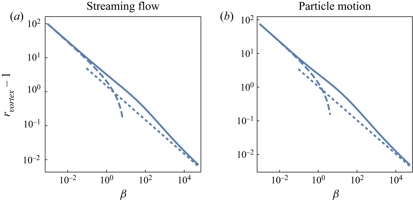
Increasing the frequency to $\beta =1$ maintains the same vortex structure and shape as for $\beta = 0.001$, in both the streaming flow and particle motion. A single vortex persists whose centre moves towards the sphere with increasing $\beta$. The radial position of the vortex centre as a function of $\beta$ is given in figure 5, along with asymptotic solutions for small and large $\beta$ obtained from the formulas in § 2.3. For small $\beta$, the corresponding asymptotic formula for the radial position of the vortex centre is

(2.22)

\begin{equation} r_{{vortex}} = \left\{\begin{array}{@{}ll} \displaystyle \dfrac{3.018634}{\sqrt{\beta}} +o \left(\dfrac{1}{\sqrt\beta} \right), & \text{streaming flow} ,\\ \displaystyle \dfrac{2.322261}{\sqrt{\beta}} +o \left(\dfrac{1}{\sqrt\beta} \right) , & \text{particle motion}, \end{array}\right. \quad \beta \rightarrow 0, \end{equation}

whereas for large $\beta$,

(2.23)

\begin{equation} r_{vortex} = \left\{\begin{array}{ll} \displaystyle 1+\dfrac{1.489040}{\sqrt\beta} +o \left(\dfrac{1}{\sqrt\beta} \right) , & \text{streaming flow} ,\\ \displaystyle 1+\dfrac{1.045580}{\sqrt\beta} +o\! \left(\dfrac{1}{\sqrt\beta} \right) , & \text{particle motion}. \end{array}\right. \quad \beta \rightarrow \infty. \end{equation}

Figure 5.

Radial distance from the sphere surface to the vortex centre, $r_{vortex} - 1$, of (a) the streaming flow and (b) the particle motion, as a function of the dimensionless frequency $\beta$. Solutions for arbitrary $\beta$ are given by (2.10) and (2.11) (solid line), for small $\beta$ by (2.22) (dashed line), and for large $\beta$ by (2.23) (dotted line). The vortex centre lies along the polar angle $\theta = 54.7356^{\circ }$ from the axis aligned with the direction of the imposed flow; see (2.10).

As the frequency is increased further to $\beta = 16$, the vortex – which occurs in the outer region of the small-$\beta$ asymptotic flow only, i.e. $r \gg \beta ^{-{1}/{2}}$ – begins to interact strongly with the sphere where the inner region resides. This interaction modifies the vortex shape leading to a blunter face near the sphere, together with a broader width. Further increasing frequency to $\beta =20$ leads to a seemingly abrupt emergence of a new counter-flow structure away from the sphere. This counter-flow emerges at an infinite distance from the sphere at a finite value of $\beta$. The radial boundary separating the inner and outer flows then approaches the sphere as $\beta$ increases. Emergence of the radial boundary between the two flow regions introduces (1) two saddle points where this boundary intersects with the $z$-axis, and (2) a ring of saddle points where it intersects with the equatorial plane (Bhosale et al. Reference Bhosale, Vishwanathan, Upadhyay, Parthasarathy, Juarez and Gazzola2022; Chan et al. Reference Chan, Bhosale, Parthasarathy and Gazzola2022). This new outer flow does not involve closed streamlines in either the streaming flow or particle motion, i.e. it does not contain an additional vortex centre. See figures 3 and 4(g–l), whose streamlines do not close in the outer region regardless the plotting domain size. This flow structure does not change as $\beta$ increases further; the only change is that the vortex near the sphere surface narrows. Note that the flow structure obtained from the exact solution for $\beta = 500$ in figures 4(k,l) bears a close resemblance to the asymptotic solution in figure 3.

2.4.3. Critical frequency for change in flow structure

Next, we determine the critical frequency $\beta \equiv \beta _{critical}$ where the above-mentioned seemingly abrupt change in flow structure occurs. The separable form of (2.10) shows that the radial position where the counter-flow emerges coincides with zero radial velocity, at non-zero angular velocity. This radial position, where the change in flow structure occurs, emerges far from the sphere and moves towards the sphere as $\beta$ increases. The radial component of the streaming flow, $u^{(1)}$, at large $r$ is

(2.24)

\begin{align} u^{(1)} &=\left\{ \frac{1}{4\,r^2}\left( \frac{\sqrt{\beta } (\sqrt{2} \beta ^3-2 \beta ^{5/2}+10 \sqrt{2} \beta ^2-72 \beta ^{3/2}+8 \sqrt{2} \beta +72 \sqrt{\beta }-144 \sqrt{2})}{1280}\right.\right. \nonumber\\ &\quad+ \left[A(\beta)\,E_1\left([1+\text{i}]\,\sqrt{\frac{\beta}{2}}\right)+ A^*(\beta)\,E_1\left([1-\text{i}]\,\sqrt{\frac{\beta}{2}}\right)\right] \nonumber\\ &\left.\left.\quad - \frac{3 \beta^3}{80}\,\mathrm{e}^{\sqrt{2\beta}}\,E_1(\sqrt{2\beta}) \vphantom{\left([1+\text{i}]\sqrt{\frac{\beta}{2}}\right)}\right) + o\left(\frac{1}{r^2}\right) \vphantom{\left([1+\text{i}]\sqrt{\frac{\beta}{2}}\right)}\right\} \left(1+3 \cos{2 \theta}\right), \end{align}

where

(2.25)

\begin{equation} A(\beta)= \frac{\beta^2}{2560}\,(1+\text{i})(10-\text{i} \beta ) \,{\rm e}^{(1+\text{i})\sqrt{{\beta}/{2}}} ([1-\text{i}] \beta +3 \sqrt{2 \beta}+3 [1+ \text{i}]). \end{equation}

The flow structure changes when this radial velocity changes sign, i.e. (2.24) vanishes, giving the required critical frequency

(2.26)

\begin{equation} \beta_{critical} = 16.317, \end{equation}

to five significant figures.

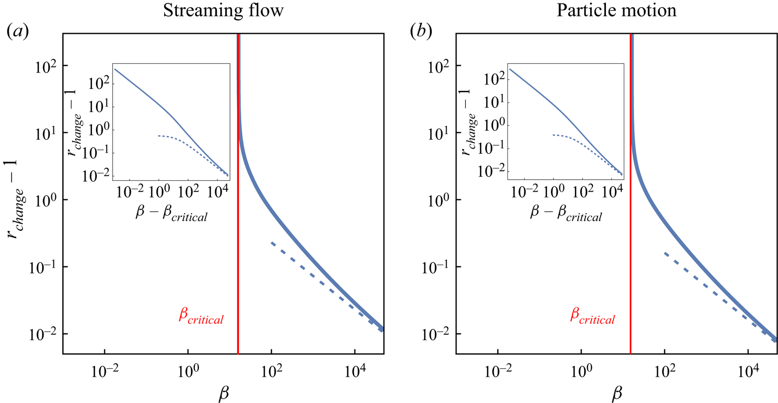
The sensitivity of this structural bifurcation near the critical frequency is illustrated by the streamlines under the selected frequency values of $\beta = 16.3$ and $\beta = 16.35$ in figure 6 – which are respectively below and above $\beta _{{critical}}$. For $\beta \approx \beta _{critical}$, the scaling law between the size of the inner region and $\beta - \beta _{{critical}}$ is plotted in the insets of figure 7.

Figure 6.

Streaming flow structure at (a) $\beta =16.3$ and (b) $\beta =16.35$. No outer region is present in (a), regardless of the size of the plotted domain. The radius of the boundary between the two regions is $r=49.542$ in (b).

Figure 7.

Radial position $r_{change}$ where the radial component of the velocity is zero as a function of $\beta$. The thickness of the inner region is $r_{change}-1$. (a) Streaming velocity field, and (b) cycle-averaged particle motion. Solutions for arbitrary $\beta$ as specified by (2.10) and (2.11) (solid line), and for large $\beta$ by (2.28) (dashed line). The red vertical line corresponds to $\beta =\beta _{{critical}}$, whose numerical value is given by (2.26). Insets show the size of the inner region versus $\beta -\beta _{{critical}}$.

As discussed in § 1, this seemingly abrupt change in flow structure also occurs for the streaming flow generated by an oscillating cylinder, which is inherently two-dimensional, in contrast to the three-dimensional flow generated by a sphere. This change in flow structure for a cylinder has been calculated theoretically (Bertelsen et al. Reference Bertelsen, Svardal and Tjøtta1973), observed experimentally (Lutz et al. Reference Lutz, Chen and Schwartz2005) and computed numerically (Parthasarathy et al. Reference Parthasarathy, Chan and Gazzola2019). Surprisingly, however, precise values for the critical frequency at which this change occurs for a cylinder have not been reported explicitly.

We define the critical dimensionless frequency for a cylinder to be $\beta _{critical}^{cyl} \equiv \omega R_{cyl}^2 / \nu$, where $R_{cyl}$ is the cylinder radius. Using this definition, figure 5 of Lutz et al. (Reference Lutz, Chen and Schwartz2005) gives an experimentally measured value $\beta _{critical}^{cyl} \approx 1/(0.15)^2 \approx 40$ – in contrast to figure 4 of Raney et al. (Reference Raney, Corelli and Westervelt1954), which produces a different experimental result, $\beta _{critical}^{cyl} \approx 4^2 \approx 16$ – while figure 2 of Bertelsen et al. (Reference Bertelsen, Svardal and Tjøtta1973) yields the theoretical prediction $\beta _{critical}^{cyl} \approx 50$. The reasons for the substantial difference between the experimental works of Raney et al. (Reference Raney, Corelli and Westervelt1954) and Lutz et al. (Reference Lutz, Chen and Schwartz2005) are unknown. However, the results for $\beta _{critical}^{cyl}$ obtained using Lutz et al. (Reference Lutz, Chen and Schwartz2005) and Bertelsen et al. (Reference Bertelsen, Svardal and Tjøtta1973) agree, and their published data have been validated independently by Parthasarathy et al. (Reference Parthasarathy, Chan and Gazzola2019). These results for $\beta _{critical}^{cyl}$ are of similar magnitude to (2.26) for a sphere, with the quantitative difference not being unexpected given their different geometries.

2.4.4. Critical frequency for streaming flow and particle motion

The radial component of the drift velocity at large $r$ is

(2.27)

\begin{equation} u_{D}^{(1)} =\left\{ \frac{9}{8 \sqrt{2 \beta}} \left(1 +\sqrt{\frac{2}{\beta}} \right)\frac{1}{r^4} + o\left(\frac{1}{r^4}\right)\right\}(1+3\cos{2\theta}), \end{equation}

which decays more rapidly with $r$ than the streaming flow $u^{(1)}$ in (2.24). It follows from (2.11) that the streaming flow and particle motion are identical far from the sphere. This feature establishes that $\beta _{critical}$ in (2.26) holds for both the streaming flow and the particle motion. That is, the critical frequency $\beta _{critical}$ can be determined by observing either flow.

2.4.5. Radial position for emergence of counter-flow

The dependence on $\beta$ of the radius $r_{change}$ at which the counter-flow emerges is given in figure 7 for both the streaming flow and particle motion. These are obtained using (2.10) and (2.11), respectively. Note that $r_{change}$ for the particle motion is smaller than that for the streaming flow. As $\beta$ approaches $\beta _{{critical}}$ from above, the asymptotic behaviour of the blue curve in figure 7 specifies a critical transition: the flow changes from a two-cell structure (figures 4g–l) to a one-cell structure (figures 4a–f). Asymptotic formulas for large $\beta$ follow directly from (2.19) and (2.21),

(2.28)

\begin{equation} r_{change} = \left\{\begin{array}{@{}ll} \displaystyle 1+\dfrac{2.3030}{\sqrt\beta} +o \left(\dfrac{1}{\sqrt\beta} \right) , & \text{streaming flow} ,\\ \displaystyle 1+\dfrac{1.6113}{\sqrt\beta} +o \left(\dfrac{1}{\sqrt\beta} \right) , & \text{particle motion}, \end{array}\right. \end{equation}

and exhibit the same $\beta$ scaling laws as for the vortex centres; cf. (2.23) and (2.28). The asymptotic results in (2.28) are also given in figure 7, and display good agreement with the exact solution for large $\beta$.

3. Finite-amplitude flows

To calculate $\beta _{{critical}}$ for finite amplitude, we perform DNS of the Navier–Stokes equations in the time domain. Specifically, the (time-averaged) streaming flow from these simulations is calculated for fixed $\epsilon$, and $\beta$ is varied to observe the transition from one to two cells; see Appendix C for details.

3.1. Dependence of $\beta _{critical}$ on oscillation amplitude

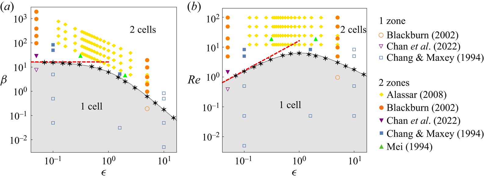
Numerical results for $\beta _{{critical}}$ as a function of oscillation amplitude $\epsilon$ are given in figure 8. Figure 8(a) reveals a universal phase space that depends only on $\beta$ and $\epsilon$, as expected from dimensional considerations; see § 1. For small amplitude $\epsilon$, finite-amplitude simulations show that $\beta _{{critical}}$ approaches the infinitesimal amplitude solution in (2.26), i.e. $\beta _{{critical}}|_{\epsilon \rightarrow 0} = 16.317$. Increasing $\epsilon$ results in a monotonic decrease in $\beta _{{critical}}$, with $\beta _{{critical}} \rightarrow 0$ as $\epsilon \rightarrow \infty$. Figure 8(b) gives the critical Reynolds number ${\textit {Re}}_{{critical}} \equiv \epsilon \,\beta _{{critical}}$, where the transition from one to two cells occurs. Fitting a cubic spline to the discrete numerical results gives a maximal value of the critical Reynolds number, ${\textit {Re}}_{{critical}} \approx 6.4$ at a dimensionless amplitude, $\epsilon = 0.95$; this small Reynolds number suppresses the onset of flow instabilities. This finding establishes that for the wide range of oscillation amplitudes studied in figure 8, i.e. $0< \epsilon \le 20$, there always exists a critical value $\beta _{{critical}}$ at which (1) transition between one and two cells occurs, and (2) the flow is laminar.

Figure 8.

Phase diagrams showing the number of cells in the streaming flow. Black asterisks are (a) the critical oscillation frequency $\beta = \beta _{{critical}}$, and (b) the critical Reynolds number ${\textit {Re}} = {\textit {Re}}_{{critical}}$, as a function of the oscillation amplitude $\epsilon$ obtained using DNS; the black curve is (3.4). Grey-shaded regions (below the black curve) correspond to one circulatory cell; white regions specify two cells. Red dashed lines are asymptotes in the small-amplitude limit; see (2.26) and (2.7). Open and solid circles correspond to one and two cells, respectively, from previous DNS studies: blue squares from table 3 of Chang & Maxey (Reference Chang and Maxey1994); orange circles from figure 11 in Blackburn (Reference Blackburn2002); green triangles from figure 6 of Mei (Reference Mei1994); purple inverted triangles from figure 2 of Chan et al. (Reference Chan, Bhosale, Parthasarathy and Gazzola2022); and yellow diamonds from table 1 of Alassar (Reference Alassar2008).

Figure 8 also shows previous numerical results for finite amplitude (Chang & Maxey Reference Chang and Maxey1994; Mei Reference Mei1994; Blackburn Reference Blackburn2002; Alassar Reference Alassar2008; Chan et al. Reference Chan, Bhosale, Parthasarathy and Gazzola2022). Importantly, Chang & Maxey (Reference Chang and Maxey1994) note: ‘There do not appear to be any generalizations that can be made for the existence of inner and outer streaming regions for flows of all amplitudes.’ This claim is explored in detail here. Filled symbols indicate two cells while open symbols indicate one circulation cell, for these previous studies. Our calculated dependence of $\beta _{{critical}}$ on $\epsilon$ captures correctly all previous numerical results, with the exception of two data points reported by Chang & Maxey (Reference Chang and Maxey1994): the two rightmost open-square symbols lying above the $\beta _{{critical}}$ versus $\epsilon$ curve in figure 8. Specifically, Chang & Maxey (Reference Chang and Maxey1994) report that these flows exhibit only one circulation cell, whereas the phase diagram in figure 8 suggests that two cells should exist.

We perform DNS of the streaming flows for these two anomalous data points, the results of which are reported in figure 9. These new simulations are converged carefully and clearly exhibit two cells, in contrast to the data reported by Chang & Maxey (Reference Chang and Maxey1994). Because the values of $\beta$ are close to $\beta _{{critical}}$ (see figure 8) – producing a counter-flow far from the sphere where the flow speed is small – it appears that numerical issues in the study of Chang & Maxey (Reference Chang and Maxey1994) are the cause of the above-mentioned discrepancy. Our new simulations provide the generalisation sought by Chang & Maxey (Reference Chang and Maxey1994) (see quote above) and show that the existence of one or two cells collapses onto a two-dimensional phase space delineated by a single curve, defined by $\beta$ and $\epsilon$.

Figure 9.

Our DNS using parameters in rows 4 and 11 of table 3 of Chang & Maxey (Reference Chang and Maxey1994), who reported one cell. In contrast, our simulations recover two cells. Respective streamlines of the streaming flow shown for (a) $\epsilon = 10$ and $\beta =0.5$, and (b) $\epsilon =10$ and $\beta =0.837$. Emergence of the counter-flow occurs at a distance approximately 20 sphere radii from the sphere surface. The $z$-axis is aligned to the direction of oscillation.

3.2. Large-amplitude limit, $\epsilon \gg 1$

Next, we consider the large-amplitude limit, $\epsilon \gg 1$, and examine the behaviour of $\beta _{critical}$ under the condition

(3.1)

\begin{equation} \beta \ll \epsilon \beta \ll 1, \end{equation}

which is justified a posteriori. The Navier–Stokes equations are both quasi-steady and quasi-linear under (3.1), with inertia exerting a small effect; i.e. the overall flow is approximately harmonic with streaming being a weak secondary flow (as for the small-amplitude limit). The Navier–Stokes equations then correspond to a weakly perturbed unsteady version of the Oseen equation for small Reynolds number flow. Balancing the linear and convective inertia terms with the diffusive viscous term, gives two length scales that are large relative to the sphere radius (scaled to unity): (1) the usual viscous penetration depth due to linear inertia, $\delta _{linear} = 1/\sqrt {\beta }$, and (2) the thickness of the viscous layer due to convective inertia, $\delta _{conv} = 1/{\textit {Re}} = 1/(\epsilon \beta )$. The relative magnitude of these two length scales controls the flow structure. Because the convective inertia term is much larger than the linear inertia term in the Navier–Stokes equations for this large-amplitude limit, the flow will resemble predominantly an Oseen flow.

To examine this further, we consider the case of fixed (large) amplitude $\epsilon$ where the frequency $\beta$ is varied. In the large-frequency limit, $1/\epsilon ^2 \ll \beta \ (\ll 1/\epsilon$, see (3.1)), where $\delta _{linear} \gg \delta _{conv}$, i.e. the streaming flow will closely resemble the Oseen flow except at distances $r \ge O( \delta _{linear} )$, where the streaming flow is small. This allows the linear inertia term in the Navier–Stokes equations to exert a significant effect. Therefore, the flow will be approximately steady close to the sphere, with unsteadiness manifesting far from the sphere, i.e. the flow will exhibit different physics near and far from the sphere. Numerical simulations support this conclusion and show two cells in this large-frequency limit; see figure 8. In the opposite limit of small frequency, $\beta \ll 1/\epsilon ^2$, where the linear viscous penetration depth is $\delta _{linear} \ll \delta _{conv}$, the linear inertia term exerts a (weak) effect precisely in the region where the streaming flow is dominated by convective inertia. Thus the flow physics is uniform through the domain and the streaming flow remains unchanged from the Oseen flow – it does not have a two-cell structure.

From these conclusions for small and large frequency, it then follows that the streaming flow must transition in its structure from one to two cells when $\delta _{linear} \sim \delta _{conv}$, which gives

(3.2)

\begin{equation} \beta_{critical} \sim \frac{1}{\epsilon^2}, \quad \epsilon \gg 1. \end{equation}

Such a monotonic decrease in $\beta _{critical}$ with increasing $\epsilon$, in the large-amplitude limit, is observed in the numerical results reported in figure 8. Equation (3.2) evidently satisfies the condition of its derivation in (3.1), as required.

The linear and convective inertia terms of the Navier–Stokes equations balance when the (dimensionless) length scale of the flow field is $\epsilon$. From the above discussion, it then follows that the inner and outer cells (when they exist) meet at a dimensionless distance from the sphere

(3.3)

\begin{equation} r \sim \epsilon, \end{equation}

in this large-amplitude and small-Reynolds-number limit. This establishes that increasing the oscillation amplitude $\epsilon$ increases the distance from the sphere at which the outer cell occurs. This theoretical prediction is borne out in numerical simulations at finite and large oscillation amplitude; see § C.1.

Finally, we note that the governing streaming flow equations in the small-amplitude limit, $\epsilon \ll 1$, contain only one length scale (in addition to the sphere radius): the viscous penetration depth $\delta _{linear}$. The Reynolds number ${\textit {Re}} \equiv \epsilon \beta$ merely dictates the strength of the streaming flow, rather than controlling its structure. Thus the above analysis for large-amplitude flows does not apply in the small-amplitude limit.

3.3. Composite arbitrary amplitude formula, $\beta _{critical}$

Combining the small-amplitude asymptotic solution for $\beta _{critical}$ in (2.26) with the large-amplitude scaling law in (3.2), using a Padé approximant, and performing a nonlinear least squares fit to the numerical data in figure 8, gives

(3.4)

\begin{equation} \beta_{{critical}} \approx \frac{16.317}{1 + 0.73\epsilon + 0.86\epsilon^2}, \end{equation}

which exhibits maximum error $5\,\%$ over the full range studied, $0<\epsilon \le 20$.

This approximate formula can be used to determine the existence of one or two cells in the streaming flow, for finite amplitude $\epsilon$. Namely, $\beta < \beta _{{critical}}$ gives one circulation cell, whereas $\beta > \beta _{{critical}}$ gives two cells. It provides the generalisation sought by Chang & Maxey (Reference Chang and Maxey1994) for the existence of one or two cells.

4. Conclusions

We have examined the secondary streaming flow generated by a stationary solid sphere immersed in an unbounded viscous fluid that is undergoing harmonic oscillation. This included formulation of an exact analytical solution in the limit of small oscillation amplitude and DNS of the Navier–Stokes equations for finite (and large) amplitude. This showed that the streaming flow exhibits two distinct topologies that depend only on the oscillation frequency $\beta$ and flow amplitude $\epsilon$.

In the small-amplitude limit, $\epsilon \ll 1$, one cell exists for frequencies $\beta < \beta _{critical} =16.317$, while two cells occur at larger frequency. This critical frequency, $\beta _{critical}$, decreases monotonically with increasing amplitude $\epsilon$, and was shown to vary as $\epsilon ^{-2}$ in the large-amplitude limit, $\epsilon \gg 1$. The conclusion of Chang & Maxey (Reference Chang and Maxey1994) that there ‘[does] not appear to be any generalisations that can be made for the existence of inner and outer streaming regions for flows of all amplitudes’ was shown to be due to numerical issues. Instead, the flow topology was found to collapse onto the $\beta$–$\epsilon$ phase space, with the existence of one or two cells being delineated by a single curve; see (3.4). Flow at the transition frequency $\beta _{critical}$ was found to always occur at small Reynolds number $\text {Re} < 6.5$, mitigating the effect of flow instabilities and ensuring laminar flow for any oscillation amplitude.

This analytical and numerical study motivates experiments to observe this phase space dependence of the flow topology, which may have implications for inertial particle trapping and transport, and the autonomous propulsion of small swimmers that are driven by secondary streaming flows (Nadal & Lauga Reference Nadal and Lauga2014; Collis, Chakraborty & Sader Reference Collis, Chakraborty and Sader2017; Zhou et al. Reference Zhou, Zhao, Wei and Wang2017; Ren, Wang & Mallouk Reference Ren, Wang and Mallouk2018; Lippera et al. Reference Lippera, Dauchot, Michelin and Benzaquen2019; Mohanty, Khalil & Misra Reference Mohanty, Khalil and Misra2020; Nadal & Michelin Reference Nadal and Michelin2020; Valdez-Garduño et al. Reference Valdez-Garduño, Leal-Estrada, Oliveros-Mata, Sandoval-Bojorquez, Soto, Wang and Garcia-Gradilla2020; Bhosale et al. Reference Bhosale, Vishwanathan, Upadhyay, Parthasarathy, Juarez and Gazzola2022; Collis, Chakraborty & Sader Reference Collis, Chakraborty and Sader2022; Li et al. Reference Li, Mayorga-Martinez, Ohl and Pumera2022).

Supplementary material

Supplementary material is available at https://doi.org/10.1017/jfm.2023.758.

Funding

The authors acknowledge support of the Melbourne Research Scholarship, the Australian Research Council grants scheme and the German Research Foundation (grant no. SCHN 1599/1-1).

Declaration of interests

The authors report no conflict of interest.

Appendix A. Analytical details of the streaming flow solution

In this appendix, we summarise briefly the derivation of $\psi ^{(1)}$, and provide the definitions of the coefficient and functions in (2.10) and (2.12). Substituting

(A1)

\begin{equation} \psi^{(1)}(r,\theta) = \xi(r)\cos{\theta}\sin^2{\theta}, \quad \psi^{(0)}(r,\theta) = \chi(r)\sin^2{\theta} \end{equation}

into (2.6), where $\chi (r)$ is the radial function of (2.9), gives the ordinary differential equation

(A2)

\begin{equation} \xi^{(4)}(r)-\frac{12 \xi''(r)}{r^2}+\frac{24 \xi'(r)}{r^3} = \kappa(r) + \kappa^{*}(r), \end{equation}

where

(A3)

\begin{equation} \kappa(r) = \beta\left(\frac{4 \chi(r)\chi^{*}(r)}{r^5}-\frac{\chi^{*}(r)\,\chi'(r)}{r^4}-\frac{\chi^{*}(r)\,\chi''(r)}{r^3} + \frac{\chi^{*}(r) \chi'''(r)}{2r^2}\right).\end{equation}

The corresponding boundary conditions are

(A4)

\begin{equation} \xi(1) = \xi'(1) = 0, \quad \lim_{r\to\infty} \left(\frac{\xi(r)}{r^2} \right) = \lim_{r\to \infty} \left(\frac{\xi'(r)}{r}\right)=0. \end{equation}

The solution to (A2)–(A4) is then

(A5)

\begin{align} \xi(r) &= f_{1} + \frac{f_{2}}{r^2} + f_{3}(r)\,E_{1}(\sqrt{2 \beta}\, r)+f_{4}(r)\,E_{1}\left((1+\mathrm{i})\,\sqrt{\frac{\beta}{2}}\, r\right)+f_{4}^{*}(r)\,E_{1}\left((1-\mathrm{i})\,\sqrt{\frac{\beta}{2}}\,r\right)\nonumber\\ &\quad+ f_{5}(r)\,\mathrm{e}^{-\sqrt{2 \beta} (r-1)} +f_{6}(r)\,{\rm e}^{-(1+\mathrm{i})\sqrt{{\beta}/{2}}(r-1)}+f_{6}^{*}(r)\,{\rm e}^{-(1-\mathrm{i})\sqrt{{\beta}/{2}}(r-1)}. \end{align}

The constants and functions in (2.10) and (A5) are

(A6a)

\begin{align} f_{1} &= \frac{\sqrt{\beta } (\sqrt{2} \beta ^3-2 \beta ^{5/2}+10 \sqrt{2} \beta ^2-72 \beta ^{3/2}+8 \sqrt{2} \beta +72 \sqrt{\beta }-144 \sqrt{2})}{2560} \nonumber\\ &\quad+ \left[\frac{A(\beta)}{2}\,E_1\left([1+\text{i}]\,\sqrt{\frac{\beta}{2}}\right)+ \frac{A^*(\beta)}{2}\,E_1\left([1-\text{i}]\,\sqrt{\frac{\beta}{2}}\right)\right]\notag\\ &\quad - \frac{3 \beta^3}{160}\,\mathrm{e}^{\sqrt{2\beta}}\,E_1(\sqrt{2\beta}),\end{align}

(A6b)

\begin{align} f_{2}&= \frac{1}{17\,920\,\beta }(720 \sqrt{2} \beta ^{3/2}- 24 \sqrt{2} \beta ^{5/2}-408 \beta ^2-6048 \beta -23\,184 \sqrt{2 \beta}-40\,320\nonumber\\ &\quad {}-58 \sqrt{2} \beta ^{7/2}-5 \sqrt{2} \beta ^{9/2}+10 \beta ^4+312 \beta ^3+240\, \mathrm{e}^{\sqrt{2 \beta}} \beta ^4\,E_1(\sqrt{2 \beta}))\nonumber\\ &\quad+\left[B(\beta)\,E_1\left([1+\text{i}]\,\sqrt{\frac{\beta}{2}}\right)+ B^{*}(\beta)\,E_1\left([1-\text{i}]\,\sqrt{\frac{\beta}{2}}\right)\right], \end{align}

(A6c)

\begin{align} f_{3}(r)&= \frac{3}{560}\,\mathrm{e}^{\sqrt{2 \beta}} \beta ^3 r^5, \end{align}

(A6d)

\begin{align} f_{4}(r) &= \frac{1+\mathrm{i}}{17\,920}\,\mathrm{e}^{(1+\text{i})\sqrt{{\beta}/{2}}}\beta ^2 ((1+\mathrm{i}) \beta +3\mathrm{i} \sqrt{2 \beta}+(-3+3\mathrm{i})) r^3 (\beta r^2+14\mathrm{i}), \end{align}

(A6e)

\begin{align} f_{5}(r) &= \frac{45\sqrt{{2}/{\beta}}-3 \sqrt{2} \beta ^{5/2} r^6+3 \beta ^2 r^5-3 \sqrt{2} \beta ^{3/2} r^4+9 \beta r^3-18 \sqrt{2 \beta} r^2+90 r}{1120 r^2}, \end{align}

(A6f)

\begin{align} f_{6}(r) &= \frac{1}{17\,920\,\beta r^2}( 20\,160+(288+288\mathrm{i}) \sqrt{2 \beta} (35 r+4)+24 \beta (280 \mathrm{i} r^2-9\mathrm{i} r+96)\nonumber\\ &\quad+ (12-12\mathrm{i} ) \sqrt{2} \beta ^{3/2} (r^2-9\mathrm{i} r+32)+(4+4 \mathrm{i} ) \sqrt{2} \beta ^{5/2} r^2 (3 r+\mathrm{i})^2\nonumber\\ &\quad-24 \beta ^2 r (2 r^2+\mathrm{i} r+3)-(1+\mathrm{i}) \sqrt{2} \beta ^{9/2} r^6+2 \beta ^4 r^5 (1-3\mathrm{i} r)\nonumber\\ &\quad+(3+3\mathrm{i}) \sqrt{2} \beta ^{7/2} r^4 (-\mathrm{i} r^2+r-4 \mathrm{i})+2 \beta ^3 r^3 (3\mathrm{i} r^2+36 r+8\mathrm{i})), \end{align}

where

(A7a)

$$\begin{gather} A(\beta) = \frac{\beta^2}{2560}\,(1+\text{i})(10-\text{i} \beta ) \,\mathrm{e}^{(1+\text{i})\sqrt{{\beta}/{2}}} ([1-\text{i}] \beta +3 \sqrt{2 \beta}+3 [1+ \text{i}]), \end{gather}$$

(A7b)

$$\begin{gather}B(\beta) = \frac{1+\mathrm{i}}{35\,840}\,\mathrm{e}^{(1+\text{i})\sqrt{{\beta}/{2}}}\beta ^2 ((1+\mathrm{i}) \beta +3\mathrm{i} \sqrt{2 \beta}+(-3+3\mathrm{i})) (5 \beta +42 \mathrm{i} ). \end{gather}$$

Evaluation of (2.12) then gives

(A8)

\begin{equation} \psi_{D} = \left\{ \frac{9 (\sqrt{2 \beta}+2)}{8 \beta r^2} +\frac{9 (\sqrt{2 \beta} r+2)}{8 \beta r^3}\,{\rm e}^{-\sqrt{2 \beta} (r-1)} + g(r) + g^{*} (r)\right\}\cos{\theta}\sin^2{\theta}, \end{equation}

where

(A9)

\begin{equation} g(r) =-\left(\frac{-6 \text{i} \beta +(9-9 \text{i}) \sqrt{2 \beta}+6 \text{i} \beta r^3+(9+9 \text{i}) \sqrt{2 \beta} r^2+18 r+18}{16 \beta r^3} \right) {\rm e}^{-(1+\text{i})\sqrt{{\beta}/{2}}(r-1)}. \end{equation}

Appendix B. Asymptotic analysis for small and large $\beta$

In this appendix, we provide asymptotic solutions for the streaming flow and resulting cycle-averaged particle velocity in the limits of small and large frequency, i.e. $\beta \ll 1$ and $\beta \gg 1$, respectively. These are obtained by solving (2.5) and (2.6), which themselves hold in the asymptotic limit of small oscillation amplitude, i.e. $\epsilon \rightarrow 0$. As such, the oscillation amplitude is always small relative to all flow length scales.

B.1. Small oscillation frequency, $\beta \ll 1$

Inspection of (2.5) for small $\beta$ reveals that the inertia term balances the viscous term at large distance, $r= O(\beta ^{-{1}/{2}})$. This singular behaviour at large distance motivates a matched asymptotic expansion of the stream function $\varPsi$ with respect to the radial coordinate. The corresponding inner and outer regions of this expansion are specified by $r \ll \beta ^{-{1}/{2}}$ and $r \gg \beta ^{-{1}/{2}}$, respectively. The principal aim is to calculate the leading-order streaming flow for small $\beta$.

B.1.1. Linear oscillatory flow

The governing equation for the linear oscillatory flow, (2.5), and its stream function $\psi ^{(0)}$, use the length scale for the inner region, i.e. the sphere radius. Consequently, we perform a regular perturbation expansion of the stream function $\psi ^{(0)}$ in small $\beta$,

(B1)

\begin{equation} \psi^{(0)} = \psi_{in,0}^{(0)}+o(1) , \end{equation}

to determine the leading-order solution in the inner region $\psi _{in,0}^{(0)}$. The required governing equation and boundary conditions for $\psi _{in,0}^{(0)}$ then follow from (2.5) and (2.3):

(B2)

\begin{equation} D^4 \psi_{in,0}^{(0)} = 0, \quad \left.\psi_{in,0}^{(0)} \right|_{r=1} = \left.\frac{\partial \psi_{in,0}^{(0)}}{\partial r} \right|_{r=1} =0. \end{equation}

The solution in the outer region is obtained by rescaling the spatial variable $r$ as above,

(B3)

\begin{equation} \rho =\sqrt{\frac{\beta}{2}}\,r , \end{equation}

which gives the rescaled stream function

(B4)

\begin{equation} \bar{\psi}^{(0)} =\frac{ \beta }{2} \,\psi^{(0)} . \end{equation}

Expanding $\bar {\psi }^{(0)}$ for small $\beta$,

(B5)

\begin{equation} \bar{\psi}^{(0)} = \bar{\psi}_{out,0}^{(0)}+\beta^{{1}/{2}} \, \bar{\psi}_{out,1}^{(0)} + o(\beta^{{1}/{2}}) , \end{equation}

and substituting (B5) into (2.5) and (2.3) gives the corresponding governing equations and boundary conditions for $\bar {\psi }_{out,0}^{(0)}$ and $\bar {\psi }_{out,1}^{(0)}$,

(B6)

\begin{equation} D_{\rho}^4 \bar{\psi}_{out,0}^{(0)} =-2\text{i} D_{\rho}^2 \bar{\psi}_{out,0}^{(0)} , \quad D_{\rho}^4 \bar{\psi}_{out,1}^{(0)} =-2\text{i} D_{\rho}^2 \bar{\psi}_{out,1}^{(0)} , \end{equation}

where $D_{\rho }^2$ is identical to (2.2a) with $r$ replaced by $\rho$, and

(B7)

\begin{equation} \left. \bar{\psi}_{out,0}^{(0)} \right|_{\rho \rightarrow \infty} \sim \frac{\rho^2}{2} \sin^2\theta, \quad\lim_{\rho\to\infty} \frac{1}{\rho^2}\,\bar{\psi}_{out,1}^{(0)} = \lim_{\rho\to\infty}\left( \frac{1}{\rho}\,\frac{\partial \bar{\psi}_{out,1}^{(0)}}{\partial \rho}\right) = 0. \end{equation}

Solving the above governing equations and matching the outer part of the inner solution ($r \gg 1$) to the inner part of the outer solution ($\rho \ll 1$) gives the required asymptotic solutions for the inner and outer regions, respectively:

(B8a)

$$\begin{gather} \psi^{(0)} = \frac{1}{4}\left(2 r^2 - 3 r + \frac{1}{r}\right) \sin^2 \theta + o(1), \end{gather}$$

(B8b)

$$\begin{gather}\bar{\psi}^{(0)} = \left(\frac{\rho^2}{2} + \frac{3}{4}\sqrt{\frac{\beta}{2}}\left[{\rm e}^{-(1-\text{i})\rho}\left(1+\text{i}+\frac{\text{i}}{\rho}\right)-\frac{\text{i}}{\rho}\right] \right)\sin^2\theta + o(\beta^{{1}/{2}}) . \end{gather}$$

The term of $O(\beta ^{{1}/{2}})$ in the outer solution $\bar {\psi }^{(0)}$ drives the leading-order streaming flow, as is evident in the next subsubsection.

B.1.2. Steady streaming flow

Accounting for the form of (2.6), we expand the first-order (streaming) flow for the inner region in small $\beta$ as

(B9)

\begin{equation} \psi^{(1)} = \beta \psi_{in,0}^{(1)}+o(\beta) , \end{equation}

Substituting (B1) and (B9) into (2.6) and (2.3) gives the governing equation and boundary condition for the streaming flow in the inner region:

(B10)

\begin{equation} D^4 \psi_{in,0}^{(1)} = \frac{9\beta}{8 r^5}\,(3 r^2-2 r^3-1)\cos{\theta}\sin^2{\theta}, \quad \left.\psi_{in,0}^{(1)} \right|_{r=1} =\left. \frac{\partial \psi_{in,0}^{(1)}}{\partial r} \right|_{r=1} = 0, \end{equation}

where $\psi _{in,0}^{(0)}$ is given in (B1) and (B8a).

The radial coordinate and stream function in the outer region are scaled as per (B3) and (B4), and expanded in small $\beta$ as

(B11)

\begin{equation} \bar{\psi}^{(1)} = \beta \, \bar{\psi}_{out,0}^{(1)}+ o(\beta). \end{equation}

Substituting (B11) and (B8b) into (2.6) and (2.3) then gives the governing equation for $\psi _{out,0}^{(1)}$,

(B12)

\begin{equation} D_{\rho}^4 \bar{\psi}_{out,0}^{(1)} =- \frac{9}{4}\,\mathrm{e}^{-\rho} \left[ \left(\frac{2}{3} +\frac{1 }{\rho}\right) \sin \rho+ \left(\frac{1}{\rho} +\frac{1}{\rho^2}\right) \cos \rho\right] \cos{\theta}\sin^2\theta, \end{equation}

and its associated boundary condition,

(B13)

\begin{equation} \lim_{\rho\to\infty} \frac{1}{\rho^2}\,\bar{\psi}_{out,1}^{(1)} = \lim_{\rho\to\infty}\left( \frac{1}{\rho}\,\frac{\partial \bar{\psi}_{out,1}^{(1)}}{\partial \rho}\right) = 0. \end{equation}

Solving these governing equations for the inner and outer regions, and matching their solutions, gives the following respective results in the inner and outer regions:

(B14a)

$$\begin{gather} \psi^{(1)} =\beta \left(-\frac{3 r^2}{32}-\frac{3}{64 r^2}+\frac{9 r}{64}+\frac{3}{64 r}-\frac{3}{64}\right)\cos\theta\sin^2\theta + o(\beta), \end{gather}$$

(B14b)

$$\begin{gather}\bar{\psi}^{(1)} = \frac{9 \beta}{16} \left( \mathrm{e}^{-\rho} \left[ \left( \frac{2}{3} +\frac{1}{\rho} \right) \sin \rho + \left(\frac{1}{\rho} +\frac{1}{\rho^2}\right) \cos \rho\right] - \frac{1}{\rho^2} \right) \nonumber\\ \times \cos{\theta}\sin^2\theta + o(\beta) . \end{gather}$$

B.1.3. Cycle-averaged particle velocity

As discussed in § 2.2, the stream function defining the (steady) cycle-averaged particle velocity includes the effects of Stokes drift. The latter follows directly from the linear oscillatory flow. In this subsubsection, we provide this leading-order stream function defining the particle motion in small $\beta$, for the inner and outer regions.

For the inner region, this particle stream function follows from (B14a), (2.11) and (2.12), giving

(B15)

\begin{equation} \psi_{particle}^{(1)} =-\frac{3 \beta}{64} \left(3 r+3-\frac{2}{r}\right) \left(1-\frac{1}{r}\right)^2 \cos\theta\sin^2\theta + o(\beta), \end{equation}

establishing that particle motion vanishes in the outer part of the inner region at $O(\beta )$. For the outer region, the Stokes drift contribution cancels (B14b) precisely to leading order in $\beta$, giving

(B16)

\begin{equation} \bar{\psi}^{(1)}_{particle} = o(\beta) . \end{equation}

B.2. Large oscillation frequency, $\beta \gg 1$

Next, we consider the complementary limit of large $\beta$, where the highest spatial derivative (viscous term) in (2.5) is seen to vanish. This leads to a predominantly inviscid flow everywhere, except near the sphere surface where the viscous term balances the inertia term to match the no-slip condition. This balance occurs for $r - 1 = O(\beta ^{-{1}/{2}})$, which defines the length scale for the viscous boundary layer near the sphere surface.

B.2.1. Linear oscillatory flow

Equation (2.5) uses the length scale for the outer region, and we expand its stream function in the small parameter $\beta ^{-1}$,

(B17)

\begin{equation} \psi^{(0)} = \psi_{out,0}^{(0)}+o(1) , \end{equation}

whose governing equation and boundary conditions follow from (2.5) and (2.3):

(B18)

\begin{equation} D^2\psi_{out,0}^{(0)}=0, \quad \psi_{out,0}^{(0)} \big|_{r \rightarrow \infty} \sim \frac{r^2}{2} \sin^2\theta. \end{equation}

The inner region uses the above-mentioned scaling for the radial coordinate, i.e.

(B19)

\begin{equation} \eta = \sqrt{\frac{\beta}{2}}\, (r-1) , \end{equation}

which gives the rescaled stream function for the inner region,

(B20)

\begin{equation} \bar{\psi}^{(0)} = \sqrt{\frac{\beta}{2}} \, \psi^{(0)} . \end{equation}

Expanding $\bar {\psi }^{(0)}$ for large $\beta$,

(B21)

\begin{equation} \bar{\psi}^{(0)} = \bar{\psi}_{in,0}^{(0)}+o(1) , \end{equation}

and substituting (B21) into (2.5) and (2.3), gives

(B22)

\begin{equation} \frac{\partial^4 \bar{\psi}_{in,0}^{(0)}}{\partial \eta^4} - 2 \text{i}\,\frac{\partial^2 \bar{\psi}_{in,0}^{(0)}}{\partial \eta^2} =0, \quad \bar{\psi}_{in,0}^{(0)} \big|_{\eta=0} = \left. \frac{\partial \bar{\psi}_{in,0}^{(0)}}{\partial \eta} \right|_{\eta=0} = 0. \end{equation}

Solving the above system of equations, matching the inner and outer solutions, gives the required results for the inner and outer regions, respectively:

(B23a)

$$\begin{gather} \bar{\psi}^{(0)} = \frac{3}{2}\left(\frac{1+\text{i}}{2}\left[\mathrm{e}^{({\rm i}-1)\eta}-1\right] + \eta\right)\sin^2\theta +o(1) , \end{gather}$$

(B23b)

$$\begin{gather}\psi^{(0)} = \frac{1}{2}\left(r^2 - \frac{1}{r}\right) \sin^2\theta + o(1) . \end{gather}$$

B.2.2. Steady streaming flow

The first-order (streaming) flow for the outer region is expanded in the small parameter, $\beta ^{-1}$ as

(B24)

\begin{equation} \psi^{(1)} = \psi_{out,0}^{(1)}+o(1) , \end{equation}

for which the governing equation and boundary condition follow from (2.6) and (2.3), giving

(B25)

\begin{equation} D^4 \psi_{out,0}^{(1)} = 0, \quad \lim_{r\to\infty}\frac{1}{r^2}\,\psi_{out,0}^{(1)} = \lim_{r\to\infty}\left(\frac{1}{r}\,\frac{\partial \psi_{out,0}^{(1)}}{\partial r}\right) = 0 . \end{equation}

Scaling the radial coordinate and stream function in the inner region according to (B19) and (B20), and expanding in $\beta ^{-{1}/{2}}$, gives

(B26)

\begin{equation} \bar{\psi}^{(1)} =\bar{\psi}_{in,0}^{(1)}+ o(1) , \end{equation}

which from (2.6) and (2.3) gives the required governing equation

(B27)

\begin{equation} \frac{\partial^4 \bar{\psi}_{in,0}^{(1)}}{\partial \eta^4}= \frac{9}{2} (-\mathrm{e}^{-2\eta}+\mathrm{e}^{-\eta}\cos{\eta}+\mathrm{e}^{-\eta}[2\eta-1]\sin{\eta})\cos\theta \sin^2\theta, \end{equation}

and the no-slip boundary condition,

(B28)

\begin{equation} \bar{\psi}_{in,0}^{(1)} \big|_{\eta=0} = \left. \frac{\partial \bar{\psi}_{in,0}^{(1)}}{\partial \eta} \right|_{\eta=0} = 0. \end{equation}

Solving these equations and matching their results gives the following stream functions for the outer and inner regions, respectively:

(B29a)

$$\begin{gather} \psi^{(1)} = \frac{45}{32}\left(1-\frac{1}{r^2}\right) \cos{\theta}\sin^2 \theta +o(1), \end{gather}$$

(B29b)

$$\begin{gather}\bar{\psi}^{(1)}= \left(-\frac{189}{32}+\frac{45}{16}\,\eta+ \frac{9}{32} \left[\mathrm{e}^{-2\eta}+20 \mathrm{e}^{-\eta}\cos{\eta}+4\mathrm{e}^{-\eta}(3+2\eta)\sin{\eta}\right]\right) \nonumber\\ \,\times \cos{\theta}\sin^2 \theta + o(1) . \end{gather}$$

B.2.3. Cycle-averaged particle velocity

The contribution from Stokes drift is now included to determine the stream function defining the cycle-averaged particle velocity. There is no contribution from Stokes drift to the outer region at leading order at $O(\beta ^{-1})$, giving the particle stream function

(B30)

\begin{equation} \psi_{particle}^{(1)} = \frac{45}{32}\left(1-\frac{1}{r^2}\right) \cos{\theta}\sin^2 \theta +o(1), \end{equation}

while Stokes drift is non-zero for the inner region, giving

(B31)

\begin{equation} \bar{\psi}_{particle}^{(1)} = \frac{9}{32} (10\eta-17 +12 \mathrm{e}^{-\eta}[\cos{\eta}+\sin{\eta}] + 5 \mathrm{e}^{-2\eta} ) \cos{\theta}\sin^2 \theta + o(1) . \end{equation}

Appendix C. Numerical simulations

Finite-amplitude simulations are performed with the finite element analysis software COMSOL Multiphysics, using the incompressible Navier–Stokes equations. An axisymmetric geometry is used with a half-circle of unitary radius representing the solid sphere and a half-circle of radius, $R_{\infty }$ representing the far-field condition. The solid sphere is held stationary with surface velocity $\boldsymbol {u} = \boldsymbol {0}$, while the uniform velocity $\boldsymbol {u} = \epsilon \cos t \, \boldsymbol {k}$, is prescribed to the outer sphere of radius $R_{\infty }$. Setting the shear viscosity to unity then enables the fluid density to act as a proxy for the dimensionless frequency parameter $\beta$; see (1.4).

To obtain the time-averaged solution, i.e. the secondary streaming flow, simulations are run for multiple periods and then time averaged over the final period. Because the radius of the inner circulation cell approaches infinity as $\beta \rightarrow \beta _{{critical}}$, it is important to check for convergence in the time-averaged solution. It can be small because the magnitude of this flow varies with the amplitude squared. Where only one cell is present, the location of the vortex centre is monitored to attain convergence. Where two cells exist, we monitor (i) the vortex centre of the inner cell, and (ii) the location of the zeros along the $z$- and $r$-axes, i.e. the boundary of the inner and outer cells. All simulations leading to the calculation of $\beta _{{critical}}$ are converged to at least 95 % with respect to these criteria.

Triangular mesh elements are used throughout the domain, with thin rectangular ‘boundary layer’ elements applied immediately adjacent to the stationary solid sphere. A maximum element side length 0.1 is used in the vicinity of the solid sphere, and maximum side length 5 far from the sphere. This gives approximately 8000 to 15 000 elements in total, depending on the domain size. Increasing the level of discretisation to approximately double the total number of elements demonstrates convergence in the above cell parameters to at least 95 %. This is checked for a small value, $\epsilon = 0.1$, i.e. where convergence is most challenging due to the small magnitude of the time-averaged solution, and also a large value, $\epsilon = 100$. Note that in both cases, mesh convergence is checked for $\beta$ above and below $\beta _{{critical}}$.

Convergence is also checked for the number of time-steps per period, and the total number of periods. Using 100 time steps per period and 40 total periods results in convergence of the above cell parameters to at least 95 %. This number of periods and time steps per period is used for all reported simulations. Even so, larger values of $\epsilon$ attain convergence before 40 periods due to the smaller value of $\beta _{{critical}}$. A relative tolerance 10$^{-4}$ in the time stepping is specified, which again results in convergence of the cell parameters to at least 95 %.

Zeroes of the radial component of the fluid velocity along the $r$-axis, and those of the axial component of the velocity along the $z$-axis, are examined to determine $\beta _{{critical}}$. A zero indicates the occurrence of two cells; otherwise, there is only one cell. The zero search is conducted for radii between 1 and $R_{\infty }/2$ because the finite computational domain can and does introduce spurious (small-amplitude) circulation cells in the neighbourhood of $R_{\infty }$ (data not shown). Determination of $\beta _{critical}$ for each fixed $\epsilon$ is conducted as follows. An initial value of $\beta$ is chosen such that two cells occur, and a second (smaller) value of $\beta$ is selected that generates only one cell. The midpoint of these two values is then simulated, generating a new range that contains $\beta _{{critical}}$; the midpoint of this new region is then simulated. This procedure is repeated until $\beta _{{critical}}$ is determined to achieve accuracy at least 95 %. The radius at which two cells meet for $\beta > \beta _{{critical}}$ increases as $\beta$ approaches $\beta _{{critical}}$. Use of a finite flow domain then ensures that numerical values for $\beta _{{critical}}$ strictly represent an upper bound (albeit accurate) estimate on the true value of $\beta _{{critical}}$.

Convergence in $\beta _{{critical}}$ additionally requires a check on the domain size; i.e. enlarging the domain should not result in a change to the minimum upper bound estimate of $\beta _{{critical}}$ of more than 5 %. A domain size $R_{\infty } = 200$ for $\epsilon < 5$, and $R_{\infty } = 400$ for $\epsilon \ge 5$, gives the required convergence in $\beta _{{critical}}$ to at least 95 %.

C.1. Large-amplitude numerical simulations

Figure 10 shows simulations performed at large amplitude. In this limit, balancing the linear and convective inertia terms of the Navier–Stokes equations reveals a characteristic length scale of order $\epsilon$; see details in § 3.2. Provided that $\beta$ is larger than but not too close to $\beta _{{critical}}$, i.e. where the size of the inner region becomes unbounded, the size of the inner region observed in the large-amplitude simulations is of $O(\epsilon )$, which is in agreement with the scaling analysis in § 3.2.

Figure 10.

Numerical simulations performed for the large amplitude: (a–c) $\epsilon = 10$, (d–f) $\epsilon = 32$, and (g–i) $\epsilon = 100$, where the dimensionless frequency, $\beta$, increases from left to right; (b,c) are identical to figure 9. All simulations are performed for $\beta > \beta _{{critical}}$ as per (3.4), to generate two cells. Plot regions are scaled to be of length $5\epsilon$, e.g. in (g–i), the plot axes span the range $x, y \in [0,500]$, highlighting the boundary between the cells that occurs at a distance $O(\epsilon )$ from the sphere.

C.2. Small-amplitude numerical simulations

The small-amplitude asymptotic solution shows that while two cells exist above the critical frequency, only one set of streamlines close, i.e. only one vortex exists in the immediate vicinity of the sphere (see figure 4). In contrast, our large-amplitude numerical simulations give two vortices (with closed streamlines) above the critical frequency (see figure 10). The large-amplitude simulations are fully converged with respect to domain size and discretisation.

However, application of our numerical scheme to the small-amplitude regime also gives two vortices above the critical frequency; in contradiction with the small-amplitude asymptotic theory. Convergence of these small-amplitude simulations with respect to domain size is problematic. Thus care should be taken when interpreting the results of full Navier–Stokes simulations in the small-amplitude limit. This is particularly true for streamlines away from the sphere where the fluid speed is small; streamlines and velocity fields in the vicinity of the sphere, including the transition between cells, are fully converged.

References

Alassar, R.S. 2008 Acoustic streaming on spheres. Intl J. Non-Linear Mech. 43 (9), 892–897.CrossRef Google Scholar

Bertelsen, A., Svardal, A. & Tjøtta, S. 1973 Nonlinear streaming effects associated with oscillating cylinders. J. Fluid Mech. 59 (3), 493–511.CrossRef Google Scholar

Bhosale, Y., Vishwanathan, G., Upadhyay, G., Parthasarathy, T., Juarez, G. & Gazzola, M. 2022 Multicurvature viscous streaming: flow topology and particle manipulation. Proc. Natl Acad. Sci. 119 (36), e2120538119.CrossRef Google Scholar PubMed

Blackburn, H.M. 2002 Mass and momentum transport from a sphere in steady and oscillatory flows. Phys. Fluids 14 (11), 3997–4011.CrossRef Google Scholar

Carlsson, F., Sen, M. & Löfdahl, L. 2004 Steady streaming due to vibrating walls. Phys. Fluids 16 (5), 1822–1825.CrossRef Google Scholar

Chan, F.K., Bhosale, Y., Parthasarathy, T. & Gazzola, M. 2022 Three-dimensional geometry and topology effects in viscous streaming. J. Fluid Mech. 933, A53.CrossRef Google Scholar

Chang, E.J. & Maxey, M.R. 1994 Unsteady flow about a sphere at low to moderate Reynolds number. Part 1. Oscillatory motion. J. Fluid Mech. 277, 347–379.CrossRef Google Scholar

Collis, J.F., Chakraborty, D. & Sader, J.E. 2017 Autonomous propulsion of nanorods trapped in an acoustic field. J. Fluid Mech. 825, 29–48.CrossRef Google Scholar

Collis, J.F., Chakraborty, D. & Sader, J.E. 2022 Autonomous propulsion of nanorods trapped in an acoustic field – corrigendum. J. Fluid Mech. 935, E1.CrossRef Google Scholar

Davidson, B.J. & Riley, N. 1971 Cavitation microstreaming. J. Sound Vib. 15 (2), 217–233.CrossRef Google Scholar

Dhara, N. 1982 The unsteady flow around an oscillating sphere in a viscous fluid. J. Phys. Soc. Japan 51 (12), 4095–4103.CrossRef Google Scholar

Dombrowski, T. & Klotsa, D. 2020 Kinematics of a simple reciprocal model swimmer at intermediate Reynolds numbers. Phys. Rev. Fluids 5 (6), 063103.CrossRef Google Scholar

Fabre, D., Jalal, J., Leontini, J.S. & Manasseh, R. 2017 Acoustic streaming and the induced forces between two spheres. J. Fluid Mech. 810, 378–391.CrossRef Google Scholar

Gemmell, B.J., Jiang, H. & Buskey, E.J. 2015 A tale of the ciliate tail: investigation into the adaptive significance of this sub-cellular structure. Proc. R. Soc. B 282 (1812), 20150770.CrossRef Google Scholar PubMed

Kaneko, A. & Honji, H. 1979 Double structures of steady streaming in the oscillatory viscous flow over a wavy wall. J. Fluid Mech. 93 (4), 727–736.CrossRef Google Scholar

Kotas, C.W., Yoda, M. & Rogers, P.H. 2006 Visualizations of steady streaming at moderate Reynolds numbers. Phys. Fluids 18 (9), 091102.CrossRef Google Scholar

Kotas, C.W., Yoda, M. & Rogers, P.H. 2007 Visualization of steady streaming near oscillating spheroids. Exp. Fluids 42 (1), 111–121.CrossRef Google Scholar

Kotas, C.W., Yoda, M. & Rogers, P.H. 2008 Steady streaming flows near spheroids oscillated at multiple frequencies. Exp. Fluids 45 (2), 295–307.CrossRef Google Scholar

Lane, C.A. 1955 Acoustical streaming in the vicinity of a sphere. J. Acoust. Soc. Am. 27 (6), 1082–1086.CrossRef Google Scholar

Li, J., Mayorga-Martinez, C.C., Ohl, C.-D. & Pumera, M. 2022 Ultrasonically propelled micro- and nanorobots. Adv. Funct. Mater. 32 (5), 2102265.CrossRef Google Scholar

Lippera, K., Dauchot, O., Michelin, S. & Benzaquen, M. 2019 No net motion for oscillating near-spheres at low Reynolds numbers. J. Fluid Mech. 866, R1.CrossRef Google Scholar

Longuet-Higgins, M.S. 1953 Mass transport in water waves. Phil. Trans. R. Soc. Lond. A 245 (903), 535–581.Google Scholar

Longuet-Higgins, M.S. 1998 Viscous streaming from an oscillating spherical bubble. Proc. R. Soc. Lond. A 454 (1970), 725–742.CrossRef Google Scholar

Lutz, B.R., Chen, J. & Schwartz, D.T. 2005 Microscopic steady streaming eddies created around short cylinders in a channel: flow visualization and Stokes layer scaling. Phys. Fluids 17 (2), 023601.CrossRef Google Scholar

Mei, R. 1994 Flow due to an oscillating sphere and an expression for unsteady drag on the sphere at finite Reynolds number. J. Fluid Mech. 270, 133–174.CrossRef Google Scholar

Mohaghar, M., Adhikari, D. & Webster, D.R. 2019 Characteristics of swimming shelled Antarctic pteropods (Limacina helicina antarctica) at intermediate Reynolds number regime. Phys. Rev. Fluids 4, 111101.CrossRef Google Scholar

Mohanty, S., Khalil, I.S.M. & Misra, S. 2020 Contactless acoustic micro/nano manipulation: a paradigm for next generation applications in life sciences. Proc. R. Soc. A 476 (2243), 20200621.CrossRef Google Scholar PubMed

Nadal, F. & Lauga, E. 2014 Asymmetric steady streaming as a mechanism for acoustic propulsion of rigid bodies. Phys. Fluids 26 (8), 082001.CrossRef Google Scholar

Nadal, F. & Michelin, S. 2020 Acoustic propulsion of a small, bottom-heavy sphere. J. Fluid Mech. 898, A10.CrossRef Google Scholar

Otto, F., Riegler, E.K. & Voth, G.A. 2008 Measurements of the steady streaming flow around oscillating spheres using three dimensional particle tracking velocimetry. Phys. Fluids 20 (9), 093304.CrossRef Google Scholar

Parthasarathy, T., Chan, F.K. & Gazzola, M. 2019 Streaming-enhanced flow-mediated transport. J. Fluid Mech. 878, 647–662.CrossRef Google Scholar

Raney, W.P., Corelli, J.C. & Westervelt, P.J. 1954 Acoustical streaming in the vicinity of a cylinder. J. Acoust. Soc. Am. 26 (6), 1006–1014.CrossRef Google Scholar

Rayleigh, Lord 1884 On the circulation of air observed in Kundt's tubes, and on some allied acoustical problems. Phil. Trans. R. Soc. Lond. 175, 1–21.Google Scholar

Ren, C., Cheng, L., Tong, F., Xiong, C. & Chen, T. 2019 Oscillatory flow regimes around four cylinders in a diamond arrangement. J. Fluid Mech. 877, 955–1006.CrossRef Google Scholar

Ren, L., Wang, W. & Mallouk, T.E. 2018 Two forces are better than one: combining chemical and acoustic propulsion for enhanced micromotor functionality. Acc. Chem. Res. 51 (9), 1948–1956.CrossRef Google Scholar PubMed

Riley, N. 1966 On a sphere oscillating in a viscous fluid. Q. J. Mech. Appl. Maths 19 (4), 461–472.CrossRef Google Scholar

Riley, N. 2001 Steady streaming. Annu. Rev. Fluid Mech. 33 (1), 43–65.CrossRef Google Scholar

Sarpkaya, T. & Storm, M. 1985 In-line force on a cylinder translating in oscillatory flow. Appl. Ocean Res. 7 (4), 188–196.CrossRef Google Scholar

Stokes, G.G. 1851 On the effect of the internal friction of fluids on the motion of pendulums. Trans. Camb. Phil. Soc. 9, 8–106.Google Scholar

Stuart, J.T. 1966 Double boundary layers in oscillatory viscous flow. J. Fluid Mech. 24 (4), 673–687.CrossRef Google Scholar

Valdez-Garduño, M., Leal-Estrada, M., Oliveros-Mata, E.S., Sandoval-Bojorquez, D.I., Soto, F., Wang, J. & Garcia-Gradilla, V. 2020 Density asymmetry driven propulsion of ultrasound-powered Janus micromotors. Adv. Funct. Mater. 30 (50), 2004043.CrossRef Google Scholar

Wang, C.-Y. 1965 The flow field induced by an oscillating sphere. J. Sound Vib. 2 (3), 257–269.CrossRef Google Scholar

Westervelt, P.J. 1953 a Acoustic streaming near a small obstacle. J. Acoust. Soc. Am. 25, 1123.CrossRef Google Scholar

Westervelt, P.J. 1953 b Hydrodynamic flow and Oseen's approximation. J. Acoust. Soc. Am. 25 (5), 951–953.CrossRef Google Scholar

Wu, J. & Du, G. 1997 Streaming generated by a bubble in an ultrasound field. J. Acoust. Soc. Am. 101 (4), 1899–1907.CrossRef Google Scholar

Wybrow, M.F., Yan, B. & Riley, N. 1996 Oscillatory flow over a circular cylinder close to a plane boundary. Fluid Dyn. Res. 18 (5), 269–288.CrossRef Google Scholar

Zhou, C., Zhao, L., Wei, M. & Wang, W. 2017 Twists and turns of orbiting and spinning metallic microparticles powered by megahertz ultrasound. ACS Nano 11 (12), 12668–12676.CrossRef Google Scholar PubMed

Table 1.Theoretical studies of the steady streaming flow generated by an oscillating sphere/cylinder.

Figure 1.Three-dimensional level sets of the stream function for the streaming flow: (a) $\beta = 0.1$, (b) $\beta = 20$. The asymptotic formulas in (2.14) and (2.19) for small and large frequency are used. Blue and red surfaces are used to guide the eye, and the sphere is shaded in grey. The black double arrow gives the direction of the oscillating far-field velocity.

Figure 2.Streamlines in the asymptotic limit of small $\beta$, to $O(\beta )$, of (a,b) inner and (c,d) outer regions of the streaming flow, using (2.13) and (2.14), respectively, for (a,c), and the cycle-averaged particle motion using (2.15) and (2.16), respectively, for (b,d). Cycle-averaged particle motion in the outer region is zero to $O(\beta )$; however, there is motion at higher order in $\beta$. The double arrow gives the direction of flow far from the stationary sphere. Red streamlines are to guide the eye.

Figure 3.Streamlines in the asymptotic limit of large $\beta$, of (a,b) inner and (c,d) outer regions of the streaming flow, using (2.19) and (2.18), respectively, for (a,c), and the cycle-averaged particle motion using (2.21) and (2.20), respectively, for (b,d). Results are shown for $\beta =500$. The black solid and dashed lines in (a,b) are the spherical boundary and the viscous boundary layer, respectively. The double arrow gives the direction of flow far from the stationary sphere.

Figure 4.Streamlines of (a,c,e,g,i,k) the streaming flow and (b,d,f,h,j,l) the particle motion for various $\beta$, using the arbitrary-$\beta$ formulas, i.e. (2.10) and (2.11). Results for $\beta$ values (a,b) 0.001, (c,d) 1, (e,f) 16, (g,h) 20, (i,j) 100, (k,l) 500. The double arrow gives the direction of flow far from the stationary sphere. Critically, the particle motion at (a,b) $\beta = 0.001$ differs from the asymptotic result in figure 2 because the arbitrary-$\beta$ formula is used here.

Figure 5.Radial distance from the sphere surface to the vortex centre, $r_{vortex} - 1$, of (a) the streaming flow and (b) the particle motion, as a function of the dimensionless frequency $\beta$. Solutions for arbitrary $\beta$ are given by (2.10) and (2.11) (solid line), for small $\beta$ by (2.22) (dashed line), and for large $\beta$ by (2.23) (dotted line). The vortex centre lies along the polar angle $\theta = 54.7356^{\circ }$ from the axis aligned with the direction of the imposed flow; see (2.10).

Figure 6.Streaming flow structure at (a) $\beta =16.3$ and (b) $\beta =16.35$. No outer region is present in (a), regardless of the size of the plotted domain. The radius of the boundary between the two regions is $r=49.542$ in (b).

Figure 7.Radial position $r_{change}$ where the radial component of the velocity is zero as a function of $\beta$. The thickness of the inner region is $r_{change}-1$. (a) Streaming velocity field, and (b) cycle-averaged particle motion. Solutions for arbitrary $\beta$ as specified by (2.10) and (2.11) (solid line), and for large $\beta$ by (2.28) (dashed line). The red vertical line corresponds to $\beta =\beta _{{critical}}$, whose numerical value is given by (2.26). Insets show the size of the inner region versus $\beta -\beta _{{critical}}$.

Figure 8.Phase diagrams showing the number of cells in the streaming flow. Black asterisks are (a) the critical oscillation frequency $\beta = \beta _{{critical}}$, and (b) the critical Reynolds number ${\textit {Re}} = {\textit {Re}}_{{critical}}$, as a function of the oscillation amplitude $\epsilon$ obtained using DNS; the black curve is (3.4). Grey-shaded regions (below the black curve) correspond to one circulatory cell; white regions specify two cells. Red dashed lines are asymptotes in the small-amplitude limit; see (2.26) and (2.7). Open and solid circles correspond to one and two cells, respectively, from previous DNS studies: blue squares from table 3 of Chang & Maxey (1994); orange circles from figure 11 in Blackburn (2002); green triangles from figure 6 of Mei (1994); purple inverted triangles from figure 2 of Chan et al. (2022); and yellow diamonds from table 1 of Alassar (2008).

Figure 9.Our DNS using parameters in rows 4 and 11 of table 3 of Chang & Maxey (1994), who reported one cell. In contrast, our simulations recover two cells. Respective streamlines of the streaming flow shown for (a) $\epsilon = 10$ and $\beta =0.5$, and (b) $\epsilon =10$ and $\beta =0.837$. Emergence of the counter-flow occurs at a distance approximately 20 sphere radii from the sphere surface. The $z$-axis is aligned to the direction of oscillation.

Figure 10.Numerical simulations performed for the large amplitude: (a–c) $\epsilon = 10$, (d–f) $\epsilon = 32$, and (g–i) $\epsilon = 100$, where the dimensionless frequency, $\beta$, increases from left to right; (b,c) are identical to figure 9. All simulations are performed for $\beta > \beta _{{critical}}$ as per (3.4), to generate two cells. Plot regions are scaled to be of length $5\epsilon$, e.g. in (g–i), the plot axes span the range $x, y \in [0,500]$, highlighting the boundary between the cells that occurs at a distance $O(\epsilon )$ from the sphere.

Li et al. supplementary material

PDF 793.4 KB

Li et al. supplementary material

File 25.4 KB

Article contents

Structure of the streaming flow generated by a sphere in a fluid undergoing rectilinear oscillation

Abstract

JFM classification

Information

1. Introduction

2. Small-amplitude flows

2.1. Analytical solution

2.1.1. Relationship to analytical formula of Dōhara (Reference Dhara1982)

2.2. Cycle-averaged particle paths

2.3. Asymptotic solutions for small and large frequency $\beta$

2.3.1. Small oscillation frequency, $\beta \ll 1$

2.3.2. Large oscillation frequency, $\beta \gg 1$

2.4. Results and discussion

2.4.1. Implications of asymptotic formulas for small and large $\beta$

2.4.2. True flow structure from arbitrary-$\beta$ formula

2.4.3. Critical frequency for change in flow structure

2.4.4. Critical frequency for streaming flow and particle motion

2.4.5. Radial position for emergence of counter-flow

3. Finite-amplitude flows

3.1. Dependence of $\beta _{critical}$ on oscillation amplitude

3.2. Large-amplitude limit, $\epsilon \gg 1$

3.3. Composite arbitrary amplitude formula, $\beta _{critical}$

4. Conclusions

Supplementary material

Funding

Declaration of interests

Appendix A. Analytical details of the streaming flow solution

Appendix B. Asymptotic analysis for small and large $\beta$

B.1. Small oscillation frequency, $\beta \ll 1$

B.1.1. Linear oscillatory flow

B.1.2. Steady streaming flow

B.1.3. Cycle-averaged particle velocity

B.2. Large oscillation frequency, $\beta \gg 1$

B.2.1. Linear oscillatory flow

B.2.2. Steady streaming flow

B.2.3. Cycle-averaged particle velocity

Appendix C. Numerical simulations

C.1. Large-amplitude numerical simulations

C.2. Small-amplitude numerical simulations

References

Li et al. supplementary material

Li et al. supplementary material

Save article to Kindle

Save article to Dropbox

Save article to Google Drive

Reply to: Submit a response

Your details

You have entered the maximum number of contributors

Conflicting interests