1. Hyper-recursive trees
Hypergraphs are generalizations of graphs. In a hypergraph, we have vertices and hyperedges consisting of collections of vertices. Also, the recursive tree is a well-studied structure; see [Reference Drmota2], [Reference Hofri and Mahmoud7], [Reference Frieze and Karoński8], and [Reference Smythe and Mahmoud15], among many other sources. In this paper we propose a generalization of recursive trees to become hypergraphs.
A hyper-recursive tree with parameter (hyperedge size)
 $\theta$
grows as follows. Initially, there are
 $\theta$
originating vertices, all labeled with 0. These
 $\theta$
vertices constitute the first hyperedge. At each subsequent step, a vertex is added to the structure. The incoming vertex chooses
 $\theta-1$
existing vertices to co-share a hyperedge. A vertex joining at time n is labeled with n. The choice of the vertices for the new hyperedge is done uniformly at random, with all subsets of vertices of size
 $\theta-1$
being equally likely. The usual recursive tree is one with the parameter
 $\theta = 2$
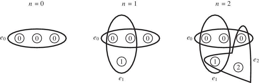
. Figure 1 illustrates the growth of a hyper-recursive tree at time
 $n=2$
. In this example
 $\theta = 3$
, and the hyperedge appearing at step i is labeled
 $e_i$
.
A hyper-recursive tree grown in two steps (
 $\theta =3$
).

Remark 1. For
 $\theta \ge 3$
, the hyper-recursive tree is not a tree at all. We call such a hypergraph by this name only to preserve the historic origin of these structures and frame them as a generalization of genuine recursive trees (
 $\theta=2$
).
2. Scope
Our interest is in a local profile of the level of containment for a vertex, which is the number of hyperedges containing it. Let
 $C_{n,k}^{(\theta)}$
be the number of hyperedges containing vertex
 $k\ge 1$
at time
 $n \ge 0$
. For instance, in the hyper-recursive tree in Figure 1, at
 $n=2$
, the vertex labeled 1 is at containment level 2, while the vertex labeled 2 is at containment level 1, and so
 $C_{2,1}^{(3)} =2$
and
 $C_{2,2}^{(3)} = 1$
. Each of the originators (all labeled with 0) may evolve differently and have different levels of containment at time n. However, the levels of these originators have the same distribution at time n, so we can choose a representative among them to include the case
 $k=0$
.
We later see that a vertex labeled
 $k = k(n)$
has an asymptotic distribution depending on the relation between k and n. Asymptotically, earlier vertices have Gaussian distributions and later vertices have shifted Poisson distributions (Theorem 3). The notions of ‘early’ and ‘late’ are made precise below, with nuances obtained from refinements into very early, early, intermediate, late, and very late vertices. We also discuss how the phases merge at the seam lines.
Moreover, we investigate a global profile of containment. Let
 $X_{n,i}^{(\theta)}$
be the number of vertices at containment level i, that is, the number of vertices contained in i edges after n evolutionary steps. For instance, in the example shown in Figure 1, we have
 $X_{2,1}^{(3)} = 1$
,
 $X_{2,2}^{(3)} = 4$
, and
 $X_{2,i} ^{(3)} = 0$
, for
 $i\ge 3$
. To get a glimpse into the interaction between different levels of containment, we compute the variance–covariance matrix of
 $(X_{n,1}^{(\theta)}, X_{n,2}^{(\theta)})$
in Theorem 4. Furthermore, we develop a Gaussian distribution for
 $X_{n,1}^{(\theta)}$
in Theorem 5.
As an outline for the rest the paper, Section 3 will cover some preliminaries and notation for later use. In Section 4 we set up a moment generating function for
 $C_{n,k}^{(\theta)}$
, from which we extract an exact distribution involving Stirling numbers of the first kind. The section contains a subsection where we portray the different phases in the asymptotic distribution.
Section 5 concerns the global containment profile. The derivation appears in incremental units. In Section 5.1 we set up a stochastic recurrence for
 $(X_{n,1}^{(\theta)}, X_{n,2}^{(\theta)})$
. In Section 5.2 we use that recurrence to find means, variances, and covariances of these two components. In Section 5.3, we quantify the asymptotic error in
 ${\mathcal{L}}_1$
, a necessary device for the martingale central limit theorem to go through. The variable
 $X_{n,1}^{(\theta)}$
is not a martingale per se: it is transformed into one in Section 5.4. The martingale central limit theorem is worked out in Section 5.5 to give a Gaussian law.
3. Notation
Let
 $\tau_n^{(\theta)}$
be the cardinality of the vertex set (size) of the hyper-recursive tree at time n (right after the insertion of vertex n). We sometimes refer to n as the age of the hyper-recursive tree. Note that
 \begin{equation}\tau_n^{(\theta)} = n + \theta.\end{equation}
The exact results are represented in terms of Pochhammer’s symbol for the rising factorial. The m-times rising factorial of a real number x is
 \begin{equation*}\langle x \rangle_m = x(x+1) \cdots (x+m-1),\end{equation*}
with the interpretation that
 $\langle x \rangle_0=1$
. We make use of such an expression in its form as a generating function of the signless Stirling numbers of the first kind, namely
 \begin{equation}\langle x \rangle_m = \sum_{i=1}^m \biggl[\begin{array}{c}m\\i\end{array}\biggr] x^i,\end{equation}
where
 $\big[\begin{array}{c}m\\[-3pt]i\end{array}\big]$
is the ith (signless) Stirling number of order m of the first kind, a count of the number of permutations of
 $\{1, 2, \ldots, m\}$
that have i cycles. For properties of Stirling numbers, we refer the reader to [Reference David and Barton1] and [Reference Graham, Knuth and Patashnik4].
Average values and variances contain generalized harmonic numbers. These are
 $H_n^{(s)} (x)$
 $= \sum_{k=1}^n 1/(k+x)^s$
, for integer
 $n\ge 0$
and real
 $s,x\ge 0$
. The superscript is often dropped when it is 1, and the number
 $H_n^{(1)}(0)$
is often written as
 $H_n$
; we follow this convention. It is well known that, for any fixed x, as
 $n \to\infty$
, we have
 \begin{align}H_n(x) = H_n^{(1)}(x) = \ln (n) - \psi(x) - \dfrac 1 x+{\mathrm{O}} \bigg(\dfrac 1 n\bigg), \end{align}
 \begin{align} H_n^{(2)}(x) = \psi(1, x+1) + {\mathrm{O}} \bigg(\dfrac 1 n\bigg),\qquad\qquad\qquad\quad\end{align}
where
 $\psi(\cdot)$
is the digamma function and
 $\psi(1,\cdot)$
is the trigamma function. Note that
 $- \psi(x) - {{1}/{x}} $
converges to Euler’s constant
 $\gamma$
, as
 $x\to 0$
.
In the asymptotic analysis, we utilize the Stirling approximation of the ratio of growing Gamma functions [Reference Tricomi and Erdélyi17]. Namely, for fixed a and b in
 $\mathbb R$
, we have
 \begin{equation}\dfrac{\Gamma(x+a)} {\Gamma(x+b)} \sim x^{a-b} \biggl(1 +\dfrac{(a-b)(a+b-1)}{2x}+ {\mathrm{O}} \biggl(\dfrac 1 {x^2} \biggr)\biggr) \quad \text{as } x \to\infty.\end{equation}
This approximation is applicable even if
 $a = a(x)$
and
 $b =b(x)$
grow slowly with x.
The sample taken at time n is drawn without replacement, and so the number of vertices in it at containment levels
 $1, \ldots, k$
have a (conditional) hypergeometric distribution. We use the notation
 $\operatorname{Hypergeo} (\tau, n_1,n_2, \ldots, n_r; s)$
for the multivariate hypergeometric random vector, in which the ith component is the number of balls of color i that appear in a sample of size s drawn from an urn containing
 $\tau$
balls, of which
 $n_i$
balls are of color i, for
 $i=1,\ldots, r$
. This multivariate hypergeometric distribution is standard and can be found in classical books on distribution theory, such as [Reference Kendall, Stuart and Ord9]. In particular, we need the mean, variances, and covariance for a bivariate marginal distribution. Suppose
 $Y_i$
is the number of balls of color i, for
 $i=1, \ldots, r$
, that appear in the sample. Then
 $(Y_i, Y_j, \tau-Y_i-Y_j)$
have a trivariate hypergeometric distribution like
 $\operatorname{Hypergeo} (\tau, n_i, n_j, \tau - n_i - n_j; s)$
, with
 $Y_i$
distributed like
 $\operatorname{Hypergeo} (\tau, n_i, \tau - n_i; s)$
. Later, we utilize the formulas
 \begin{align*}{\mathbb E}[Y_i] &= \dfrac {n_i} \tau \, s,\\\operatorname{Var}[Y_i] &= \dfrac {n_i(\tau-n_i)(\tau-s)} {\tau^2(\tau-1)} \, s,\\\operatorname{Cov}[Y_i, Y_j] &= - \dfrac {n_i n_j(\tau-s)} {\tau^2(\tau-1)} \, s;\end{align*}
see [Reference Kendall, Stuart and Ord9].
For two random variables X and Y, with induced measures
 $\mathbb P$
and
 $\mathbb Q$
, respectively, on the real line, we define the total variation distance between the two random variables (or rather between their measures) by
 \begin{equation*}d_{TV}(X,Y) =\sup_{A\in \mathcal{B}}\, \vert {\mathbb P}( A) -\mathbb Q(A) \vert, \end{equation*}
where A is an element of the Borel sigma algebra
 $\mathcal{B}$
on
 $\mathbb{R}$
. For a sequence of random variables in
 $\mathbb{N}_0$
, convergence in total variation distance is equivalent to convergence in distribution [Reference Gut5].
To derive limit distributions with rates of convergence, we use the following version of Chen–Stein approximation [Reference Ross13].
Theorem 1. Let
 $X_{1},\ldots,X_{n}$
be independent Bernoulli random variables with
 ${\mathbb P}( X_{i}=1) =p_{i}$
,
 $i=1,2,\ldots,n$
. Let
 $S_n$
be the sum
 $\sum_{i=1}^{n}X_{i}$
and
 $\lambda_n ={\mathbb E}[S_n] = \sum_{i=1}^{n}p_{i}$
. We then have
 \begin{equation*}d_{TV} (S_n,\operatorname{Poi} ( \lambda_n)) \le \min \biggl\{ 1,\dfrac{1}{\lambda_n}\biggr\} \sum_{i=1}^{n}p_{i}^{2}. \end{equation*}
A useful agent for proofs based on the Poisson approximation is the following.
Lemma 1. (See [Reference Lyon and Mahmoud10].) If
 $b>a$
and X and Y, respectively, are distributed like
 $ \operatorname{Poi}(b)$
and
 $\operatorname{Poi}(a)$
, then we have
 \begin{equation*}d_{TV}(X,Y) \le b-a. \end{equation*}
To develop martingale differences, we use the backward difference operator
 $\nabla$
. Acting on a function
 $h_n$
, this operator stands for
 $\nabla h_n = h_n- h_{n-1}$
.
4. Local containment profile
Let
 ${\mathbb I}_{n,k}^{(\theta)}$
be an indicator of the event that vertex n chooses vertex k in the hyperedge appearing at time n. The indicator
 ${\mathbb I}_{n,k}^{(\theta)}$
is a Bernoulli random variable that assumes the value 1 with probability
 \begin{equation*} \left(\begin{array}{c}\tau_{n-1}^{(\theta)}-1\\[3pt]{\theta -2}\end{array}\right)/\left(\begin{array}{c}\tau_{n-1}^{(\theta)}\\[3pt]{\theta -1}\end{array}\right) = (\theta-1)/\tau_{n-1}^{(\theta)}. \end{equation*}
This indicator has the moment generating function
 \begin{equation}\psi_{n,k}^{(\theta)} (t) \,:\!=\, {\mathbb E}\bigl[{\mathrm{e}}^{{\mathbb I}_{n,k}^{(\theta)}t}\bigr] = 1- \dfrac {\theta-1} {\tau_{n-1}^{(\theta)}} + \dfrac {(\theta-1) {\mathrm{e}}^t} {\tau_{n-1}^{(\theta)}}.\end{equation}
Adding the indicators’ contributions to
 $C_{n,k}$
across the various stages from when vertex k appears up to time n, we get the representation
 \begin{equation}C_{n,k}^{(\theta)} = 1 + {\mathbb I}_{k+1, k}^{(\theta)} + {\mathbb I}_{k+2,k} ^{(\theta)}+ \cdots+ {\mathbb I}_{n,k}^{(\theta)}\end{equation}
as independent (but not identically distributed) indicator random variables. Recall that when
 $k=0$
, we are tracking a chosen representative among the originators (all labeled with 0).
Proposition 1. Let
 $C_{n,k}^{(\theta)}$
be the containment level of the vertex labeled
 $k\ge 0$
in a hyper-recursive tree of edge size
 $\theta$
at age n. We have
 \begin{align*}{\mathbb E}\bigl[C_{n,k}^{(\theta)}\bigr] &= 1 + (\theta-1) (H_n (\theta-1) - H_k (\theta-1)) \\[5pt] &= \begin{cases}(\theta-1)\biggl(\!\ln (n) -\psi(\theta-1) - \dfrac 1 {\theta -1}\biggr) \\[13pt] \quad + 1 - (\theta-1) H_k (\theta-1) + {\mathrm{O}} \biggl(\dfrac 1 n\biggr) & if \ \text{$ k \ge 0 $}\ is\ fixed,\\[9pt] (\theta-1) \ln \biggl(\dfrac n k \biggr) + 1 + {\mathrm{O}} \biggl(\dfrac 1 k\biggr) & if \ \text{$n \ge k\to \infty$.}\end{cases}\end{align*}
and
 \begin{align*}\operatorname{Var}\bigl[C_{n,k}^{(\theta)}\bigr] &= (\theta-1) (H_n(\theta-1) - H_k (\theta-1) ) - (\theta-1)^2 (H_n^{(2)} (\theta-1) - H_k^{(2)} (\theta-1) ) \\ &= \begin{cases}(\theta-1) \ln (n) + {\mathrm{O}} (1) & if\ \text{$ k \ge 0 $}\ is\ fixed,\\[6pt] (\theta-1) \ln \biggl(\dfrac n k \biggr) + {\mathrm{O}} \biggl(\dfrac 1 k\biggr) & if\ \text{$ n\ge k\to \infty$.}\end{cases}\end{align*}
Proof. Taking expectations of (7), we find
 \begin{align*}{\mathbb E}\bigl[C_{n,k}^{(\theta)}\bigr] &= 1 + {\mathbb E}\bigl[{\mathbb I}_{k+1, k}^{(\theta)}\bigr] + {\mathbb E}\bigl[{\mathbb I}_{k+2,k}^{(\theta)}\bigr] + \cdots+ {\mathbb E}\bigl[{\mathbb I}_{n,k}^{(\theta)}\bigr]\\ &= 1 + \sum_{i=k+1}^n \dfrac {\theta-1} {\tau_{i-1}^{(\theta)}}\\ &= 1+ (\theta-1)\sum_{i=k+1}^n \dfrac 1 {i-1 + \theta}\\ &= 1 + (\theta-1) (H_n (\theta-1) - H_k (\theta-1)).\end{align*}
The asymptotic average follows from the approximation in (3).
By the independence of the indicators in (7), we similarly have
 \begin{align*}\operatorname{Var}\bigl[C_{n,k}^{(\theta)}\bigr] &= \sum_{i=k+1}^n \operatorname{Var}\bigl[{\mathbb I}_{n,k}^{(\theta)}\bigr] \\ &= \sum_{i=k+1}^n \dfrac {\theta-1} {i + \theta-1} - \sum_{i=k+1}^n \dfrac {(\theta-1)^2} {(i + \theta-1)^2}\\ &= (\theta-1)(H_n (\theta-1) - H_k (\theta-1)) - (\theta-1)^2 (H_n^{(2)}(\theta-1) - H_k^{(2)}(\theta-1)).\end{align*}
The asymptotic variance follows from the approximations in (3) and (4).
Lemma 2. The moment generating function
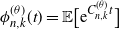 $\phi_{n,k}^{(\theta)}(t) = {\mathbb E}\bigl[{\mathrm{e}}^{C_{n,k}^{(\theta)}t}\bigr]$
of
 $C_{n,k}^{(\theta)}$
is given by
 \begin{equation*}\phi_{n,k}^{(\theta)} (t)= {\mathrm{e}}^t \prod_{i=k}^{n-1} \dfrac {i + 1 + (\theta-1){\mathrm{e}}^t}{i+\theta}. \end{equation*}
Proof. The representation (7) as a sum of independent random variables gives rise to
 \begin{align*}\phi_{n,k}^{(\theta)}(t) &= {\mathbb E}\bigl[{\mathrm{e}}^{C_{n,k}^{(\theta)}t}\bigr] \\ &= {\mathbb E}\bigl[{\mathrm{e}}^{( 1 + {\mathbb I}_{k+1, k}^{(\theta)} + {\mathbb I}_{k+2,k} ^{(\theta)} + \cdots+ {\mathbb I}_{n,k}^{(\theta)})t} \bigr]\\ &= {\mathrm{e}}^t \, \psi_{k+1, k}^{(\theta)}(t)\, \psi_{k+2, k}^{(\theta)}(t) \cdots \, \psi_{n, k}^{(\theta)}(t) \quad \text{(by independence)}.\end{align*}
Plug in (6) and the sizes of the hyper-recursive trees in (1), and the statement follows after simplification.
From Lemma 2, we develop an exact distribution.
Theorem 2. For
 $n\ge 1$
and
 $0\le k \le n$
, let
 $C_{n,k}^{(\theta)}$
be the level of containment of the vertex k in a hyper-recursive tree with edge size
 $\theta$
at age n. For
 $r\ge 1$
, we have
 \begin{equation*}{\mathbb P}(C_{n,k}^{(\theta)} = r) = \dfrac {(\theta-1)^{(r-1)}} {\langle k +\theta \rangle_{n-k}} \sum_{i=r-1}^{n-k} \biggl[\begin{array}{c}n-k\\i\end{array}\biggr] \left(\begin{array}{c}i\\r-1\end{array}\right) (k+1)^{i-r+1}.\end{equation*}
Proof. To obtain a probability generating function
 $\zeta_{n,k}^{(\theta)}(u) = \sum_{i=0}^\infty {\mathbb P}(C_{n,k}^{(\theta)} = i) u^i $
, we substitute
 $\ln(u)$
for t in the generating function of Lemma 2. We obtain
 \begin{align*}\zeta_{n,k}^{(\theta)} (u) &= u\, \dfrac { (k+1 + (\theta-1) u)\ldots( n + (\theta-1) u)} {(k+\theta) \cdots (n+\theta-1)} \\[5pt] &= u\, \dfrac {\langle k+1 +(\theta-1)u \rangle_{n-k}} {\langle k +\theta \rangle_{n-k}} .\end{align*}
Using the generating function (2), we write
 \begin{align*} \zeta_{n,k}^{(\theta)} (u) &= \dfrac u {\langle k +\theta \rangle_{n-k}} \sum_{i=0}^{n-k} \biggl[\begin{array}{c}n-k\\i\end{array}\biggr](k+ 1 + (\theta-1)u)^i \\ &= \dfrac u {\langle k +\theta \rangle_{n-k}} \sum_{i=0}^{n-k}\biggl[\begin{array}{c}n-k\\i\end{array}\biggr] \sum_{m=0}^i (k+ 1)^{i-m} (\theta-1)^m u^m \left(\begin{array}{c}i\\m\end{array}\right)\\ &= \dfrac u {\langle k +\theta \rangle_{n-k}} \sum_{m=0}^{n-k} (\theta-1)^m u ^m \sum_{i=m}^{n-k} \biggl[\begin{array}{c}n-k\\i\end{array}\biggr] \left(\begin{array}{c}i\\m\end{array}\right) (k+1)^{i-m} . \end{align*}
The exact distribution in the statement of the theorem follows upon extracting coefficients.
4.1. Phases in the local containment profile of a vertex
Proposition 1 shows that the mean and variance of
 $C_{n,k}^{(\theta)}$
experience a phase change, as k increases relative to n. For instance, for fixed k, the mean is asymptotic to
 $(\theta-1) \ln (n)$
, as
 $n\to \infty$
, and k can only alter lower-order asymptotics. However, a phase transition occurs when k grows to infinity with n but remains
 ${\mathrm{o}} (n)$
, such as the case
 $k = k(n) = \lceil 3 n^{{{3}/{4}} } + 2 \sqrt n - \pi \rceil$
. In this range, k provides essential leading-term asymptotics. The vertices that appear in the entire range in which
 $k = {\mathrm{o}} (n)$
are ‘early’.
For the linear ‘intermediate’ range,
 $k \sim \alpha n$
, for
 $0 < \alpha < 1$
, such as the case
 $\lceil \frac 5 7 n + 3\sqrt n + 6e\rceil$
, the asymptotic mean is
 $1 + (\theta-1) \ln ({{1}/{\alpha }} )$
. Vertices in the range
 $k \sim n$
are considered ‘late’. The asymptotic mean of late vertices is just 1, showing that the late arrivals, such as the case
 $k = \lfloor n - 5\ln (n+1) + 14\rfloor$
, have negligible probability of participating in the recruiting events.
It is possible to conceive of a bizarre relation between k and n, such as
 \begin{equation*}k= \biggl\lfloor \biggl(\dfrac 1 2+ \dfrac {(-1)^n} 3\biggr) n \biggr\rfloor,\end{equation*}
for which the mean containment level oscillates without settling on any asymptotic average. In these cases we have no convergence in the mean, variance, or distribution. Such an oscillating case is not likely to appear in practice.
Theorem 3. Let
 $0\le k \le n$
and let
 $C_{n,k}^{(\theta)}$
be the containment level of the vertex k in a hyper-recursive tree with edge size
 $\theta$
at age n. We have the following.
-
(i) For k fixed,
 \begin{equation*}\dfrac{C_{n,k}^{(\theta)} - (\theta-1) \ln (n)} {\sqrt {\ln (n)}} \ {\buildrel {\mathcal{D}} \over \longrightarrow}\ {\mathcal{N}} (0,\theta-1). \end{equation*}
-
(ii) For
$k\to \infty$
and
$k = {\mathrm{o}} (n)$
,
\begin{equation*}\dfrac{C_{n,k}^{(\theta)} - (\theta-1) \ln ({{n}/{k}} )} {\sqrt {\ln ({{n}/{k}} )}} \ {\buildrel {\mathcal{D}} \over \longrightarrow} \ {\mathcal{N}} (0,\theta-1). \end{equation*}
-
(iii) For
$k\sim \alpha n$
and
$0 < \alpha < 1$
,
\begin{equation*}C_{n,k}^{(\theta)} \ \ {\buildrel {\mathcal{D}} \over \longrightarrow}\ \ 1 + \operatorname{Poi} \biggl((\theta-1) \ln \biggl(\dfrac 1 \alpha\biggr)\biggr).\end{equation*}
-
(iv) For
$k = n- {\mathrm{o}} (n)$
,
\begin{equation*}C_{n,k}^{(\theta)} \ \buildrel {\mathcal{P}} \over \longrightarrow \ 1.\end{equation*}


Proof. With
 $k_n = {\mathrm{o}} (n)$
in parts (i) and (ii),
 $C_{n,k}^{(\theta)}-1$
is the sum of an increasing number of indicators (see (7)), and the variance of
 $C_{n,k}^{(\theta)}$
increases with n without bound. So
 $C_{n,k}^{(\theta)}$
is amenable to Lindeberg’s central limit theorem, as stated.
Part (iii) is amenable to Chen–Stein Poisson approximation. This line can also give us the rate of convergence in total variation distance, an added advantage. Consider the range
 $k_n \sim \alpha n$
, for
 $\alpha \in (0,1]$
. Set
 $\lambda = (\theta-1) \ln (1/\alpha)$
. In our context, we have
 \begin{equation}d_{TV}\bigl(C_{n,k}^{(\theta)} -1, \operatorname{Poi}(\lambda)\bigr) \le d_{TV}\bigl(C_{n,k}^{(\theta)}-1 , \operatorname{Poi}(\lambda_n)\bigr)+ d_{TV}\bigl(\operatorname{Poi}(\lambda_n) , \operatorname{Poi}(\lambda)\bigr).\end{equation}
Proposition 1 states that
 $\tau_n$
is of order
 $\ln n$
. We have
 $\tau_n \ge 1$
for all
 $n\ge 0$
. Theorem 1 and the asymptotic equivalent in (4) give us
 \begin{align*}d_{TV}\bigl(C_{n,k}^{(\theta)}-1 , \operatorname{Poi}(\lambda_n)\bigr) &\le\dfrac{1} {\lambda_n}\sum_{i=k}^{n-1} \dfrac {(\theta-1)^2} {(i+\theta)^2} = {\mathrm{O}} \biggl(\dfrac 1 {\ln n} \biggr) \times {\mathrm{O}} \biggl(\dfrac 1 n\biggr) = \biggl(\dfrac 1 {n\ln n}\biggr).\end{align*}
Lemma 1 asserts that
 \begin{equation*}d_{TV}(\operatorname{Poi}(\lambda_n), \operatorname{Poi}(\lambda)) \le |\lambda_n - \lambda| = \biggl|\sum_{i=k}^{n-1} \dfrac {\theta-1} {i +\theta} - (\theta-1)\ln \biggl(\dfrac 1 \alpha\biggr)\biggr|.\end{equation*}
The asymptotic approximation (3) simplifies this upper bound to
 \begin{equation*}d_{TV}(\operatorname{Poi}(\lambda_n) , \operatorname{Poi}(\lambda)) \le (\theta-1) \biggl|\ln(n)+ {\mathrm{O}} \biggl(\dfrac 1 n\biggr) - \biggl( \ln(k) + {\mathrm{O}} \biggl(\dfrac 1 k\biggr) \biggr) - \ln \biggl(\dfrac 1 \alpha\biggr)\biggr|,\end{equation*}
which is
 ${\mathrm{O}} (1/n)$
. The sum of the two terms on the right-hand side of (8) is
 ${\mathrm{O}} (1/n)$
. This establishes part (iii), with
 ${\mathrm{O}} (1/n)$
rate of convergence in total variation distance.
Then
 $C_{n,k}^{(\theta)}$
degenerates to a constant in the case
 $\alpha =1$
, where we get
 $C_{n,k}^{(\theta)} \ {\buildrel {\mathcal{D}} \over \longrightarrow}\ 1$
. Convergence in distribution to a constant implies convergence in probability, as stated in part (iv) of the theorem.
Remark 2. Phase changes of the type in Theorem 3 have been observed in [Reference Feng, Mahmoud and Panholzer3] and [Reference Mahmoud11].
Remark 3. At the seam lines between the phases, the change is not abrupt. In fact, the phases ‘flow into each other’ in a natural way, and the role of k is negligible, so long as
 $\ln (k) = {\mathrm{o}} (\sqrt{ \ln (n)}\,)$
. Past this threshold,
 $\ln (k)$
cannot be neglected relative to
 $\sqrt{ \ln (n)}$
, and k must be included in the convergence. Again, the limit in part (iii) converges to that in part (iv), as
 $\alpha \to 1$
.
We conclude this section by noting that Theorem 3 can be derived in a number of different ways. We systematically used the moment generating function to derive the exact distribution and all the parts of Theorem 3. Parts (i) and (ii) of Theorem 3 are amenable to Lindeberg’s central limit theorem, since all the indicators in (7) are bounded and the variance of
 $C_{n,k}^{(\theta)}$
increases with n without a bound.
Part (iii) is amenable to Chen–Stein Poisson approximation. This line can also give us the rate of convergence in total variation distance, an added advantage. We denote such a distance between the measures of X and Y by
 $d_{TV} (X,Y)$
. We outline this argument to find a
 ${\mathrm{O}} (1/n)$
rate.
5. Global containment profile
In this section we look at a profile of the hyper-recursive tree determined by a raw count of the number of vertices at a particular containment level. Such a profile is global, as it cannot be determined without looking at all the vertices in the entire hyper-recursive tree.
We defined
 $X_{n,i}^{(\theta)}$
to be the number of vertices contained in exactly i hyperedges. To discern how the different containment levels interact, we investigate the mean of the row vector
 $(X_{n,1}^{(\theta)}, X_{n,2}^{(\theta)})$
and its covariance matrix.
We start with stochastic recurrences, from which we proceed to a calculation of the exact mean and variances, which lead us to concentration laws. Finally we establish a central limit theorem for the vertices at the smallest level of containment, i.e. the vertices contained in one hyperedge.
5.1. Stochastic recurrences
We discuss here recurrence equations that hold on the stochastic path. Let
 $Q_{n,i}^{(\theta)}$
be the number of vertices at containment level
 $i=1,2$
that appear in the sample chosen to construct the nth hyperedge. The row vector
 \begin{equation*}\bigl(Q_{n,1}^{(\theta)}, Q_{n,2}^{(\theta)}, \tau_{n-1}^{(\theta)} - Q_{n,1}^{(\theta)}- Q_{n,2}^{(\theta)}\bigr)\end{equation*}
has a (conditional) trivariate hypergeometric distribution that selects a sample of size
 $\theta-1$
from among
 $\tau_{n-1}^{(\theta)}$
vertices, of which
 $X_{n,i}^{(\theta)}$
are at containment level i, for
 $i=1, 2$
. That is, the components of this row vector have the conditional joint distribution
 \begin{equation*}{\mathbb P}\bigl(Q_{n,1}^{(\theta)} =q_1, Q_{n,2}^{(\theta)}=q_2 \mid X_{n-1,1}^{(\theta)}, X_{n-1,2}^{(\theta)}\bigr) = \dfrac{\left(\begin{array}{c}X_{n-1,1}^{(\theta)}\\q_1\end{array}\right)\left(\begin{array}{c}X_{n-1,2}^{(\theta)}\\q_2\end{array}\right)\left(\begin{array}{c}\tau_{n-1}^{(\theta)} - X_{n-1,1}^{(\theta)} - X_{n-1,2}^{(\theta)} \\\theta -1 - q_1 - q_2\end{array}\right)}{\left(\begin{array}{c}\tau_{n-1}^{(\theta)} \\\theta-1\end{array}\right)}.\end{equation*}
The conditional means, variances, and covariance are specified in Section 3.
In the construction of the nth hyperedge, each vertex at containment level 1 in the sample upgrades to containment level 2, and the newly added vertex at step n is at containment level 1. Thus we have the stochastic recurrence
 \begin{equation}X_{n,1}^{(\theta)} = X_{n-1,1}^{(\theta)} - Q_{n,1}^{(\theta)} + 1.\end{equation}
Likewise, each vertex at containment level 2 in the sample upgrades to containment level 3. However, the
 $Q_{n,1}^{(\theta)}$
vertices at containment level 1 in the sample all move to containment level 2, giving rise to the stochastic recurrence
 \begin{equation}X_{n,2}^{(\theta)} = X_{n-1,2}^{(\theta)} - Q_{n,2} ^{(\theta)}+ Q_{n,1}^{(\theta)}.\end{equation}
5.2. The mean and covariance matrix
The pair of stochastic equations (9) and (10) is sufficient to determine the means exactly and the quadratic order moments asymptotically.
Proposition 2. Let
 $X_{n,i}^{(\theta)}$
be the number of vertices contained in exactly i hyperedges, for
 $i=1,2$
, of a recursive hyper-recursive tree of edge size
 $\theta$
. We have the mean vector
 \begin{align*}\begin{pmatrix} {\mathbb E}\bigl[X_{n,1}^{(\theta)}\bigr]\\[3pt] {\mathbb E}\bigl[X_{n,2}^{(\theta)}\bigr] \end{pmatrix} &= \begin{pmatrix} \displaystyle \dfrac 1 \theta\, n + 1 + (\theta-1) \, \Gamma (\theta) \dfrac {\Gamma(n+1)}{ \Gamma(n+\theta)} \\[10pt] \displaystyle \dfrac {(\theta-1)} {\theta^2} ( n + \theta) + \Gamma (\theta) \dfrac {\Gamma(n+1)}{ \Gamma(n+\theta)} \biggl((\theta-1)^2 H_n - \dfrac {\theta -1} \theta \biggr) \end{pmatrix} \\[6pt] &= \begin{pmatrix} \displaystyle \dfrac n \theta +1+ {\mathrm{O}} \biggl(\dfrac 1 {n^{\theta-1}} \biggr) \\[10pt] \displaystyle \dfrac {(\theta-1)} {\theta^2} ( n + \theta) + {\mathrm{O}} \biggl(\dfrac {\ln (n)} {n^{\theta-1}}\biggr) \end{pmatrix}\!.\end{align*}
Proof. Let
 ${\mathbb F}^{(\theta)}_n$
be the sigma field generated by the first n hyperedge additions. Conditioning the stochastic relations (9) and (10) on
 ${\mathbb F}^{(\theta)}_{n-1}$
, we obtain
 \begin{align*}{\mathbb E}\bigl[X_{n,1}^{(\theta)} \mid {\mathbb F}^{(\theta)}_{n-1}\bigr] \,=\,& X_{n-1,1} - {\mathbb E}\bigl[Q_{n,1}^{(\theta)} \mid {\mathbb F}^{(\theta)}_{n-1}\bigr] + 1,\\[5pt]{\mathbb E}\bigl[X_{n,2}^{(\theta)} \mid {\mathbb F}^{(\theta)}_{n-1}\bigr] \,=\,& X_{n-1,2}^{(\theta)} - {\mathbb E}\bigl[Q_{n,2}^{(\theta)} \mid {\mathbb F}^{(\theta)}_{n-1}\bigr] + {\mathbb E}\bigl[Q_{n,1}^{(\theta)} \mid {\mathbb F}^{(\theta)}_{n-1}\bigr].\end{align*}
As discussed, the random variables
 $Q_{n,1}^{(\theta)}$
,
 $Q_{n,2}^{(\theta)}$
, and
 $\tau_{n-1}^{(\theta)} - Q_{n,1}^{(\theta)} - Q_{n,2}^{(\theta)}$
have a (conditional) trivariate hypergeometric marginal distribution; the conditional expectations are
 \begin{align}{\mathbb E}\bigl[X_{n,1}^{(\theta)} \mid {\mathbb F}^{(\theta)}_{n-1}\bigr] &= X_{n-1,1}^{(\theta)} -\dfrac {X_{n-1,1}^{(\theta)}}{\tau_{n-1}^{(\theta)}} (\theta-1) +1, \qquad\qquad\end{align}
 \begin{align}{\mathbb E}\bigl[X_{n,2}^{(\theta)} \mid {\mathbb F}^{(\theta)}_{n-1}\bigr] &= X_{n-1,2}^{(\theta)} -\dfrac {X_{n-1,2}}{\tau_{n-1}^{(\theta)}} (\theta-1) + \dfrac {X_{n-1,1}^{(\theta)}}{\tau_{n-1}^{(\theta)}} (\theta-1);\notag\end{align}
see the formulas in Section 3. Taking an iterated average, simultaneous recurrences can be written as
 \begin{align}{\mathbb E}\bigl[X_{n,1}^{(\theta)}\bigr] &= \biggl(1- \dfrac {\theta-1} {\tau_{n-1}^{(\theta)}} \biggr) {\mathbb E}\bigl[X_{n-1,1}^{(\theta)}\bigr] +1 = \dfrac n {n+\theta-1} {\mathbb E}\bigl[X_{n-1,1}^{(\theta)}\bigr] +1,\end{align}
 \begin{align}{\mathbb E}\bigl[X_{n,2}^{(\theta)}\bigr] &= \biggl(1 -\dfrac {\theta-1} {\tau_{n-1}^{(\theta)}}\biggr) {\mathbb E}\bigl[X_{n-1,2}^{(\theta)}\bigr] + \dfrac {\theta-1}{\tau_{n-1}^{(\theta)}} {\mathbb E}\bigl[X_{n-1,1}^{(\theta)}\bigr] \notag\\[4pt] & = \dfrac n {n+\theta-1} {\mathbb E}\bigl[X_{n-1,2}^{(\theta)}\bigr] + \dfrac {\theta-1}{n + \theta-1} {\mathbb E}\bigl[X_{n-1,1}^{(\theta)}\bigr].\qquad\qquad\quad\end{align}
The first of these two equations is self-contained, while the second has to wait for the solution of the first to be bootstrapped into it. The first equation has the standard form
 \begin{equation}y_n = g_n y_{n-1} + h_n,\end{equation}
with solution
 \begin{equation*}y_n = \sum_{i=1}^n h_i\prod_{j=i+1}^n g_j + y_0 \prod_{j=1}^n g_j. \end{equation*}
We solve (12), with
 $g_n ={{n}/{(n+\theta-1)}}$
and
 $h_n =1$
, and obtain
 \begin{align*}{\mathbb E}\bigl[X_{n,1}^{(\theta)}\bigr] &= \sum_{i=1}^n \prod_{j=i+1}^n \dfrac j {j+\theta-1} + \theta \prod_{j=1}^n \dfrac j {j+\theta-1} \\ &= \dfrac {\Gamma(n+1)} {\Gamma(n+\theta)} \sum_{i=1}^n \dfrac {\Gamma(i+\theta)} {\Gamma(i+1)} + \dfrac {\theta\, \Gamma(\theta)\, \Gamma(n+1)} {\Gamma(n+\theta)}.\end{align*}
To simplify the sum, we use a known identity, which is namely
 \begin{align}\sum_{i=1}^n\dfrac{\Gamma(i+\alpha)}{\Gamma(i+\beta)}&= \dfrac{ \Gamma(n+\alpha+1)}{(\alpha-\beta +1)\Gamma(n+\beta)} - \dfrac{ \Gamma(\alpha+1)}{(\alpha-\beta +1)\Gamma(\beta)},\end{align}
for any given
 $\alpha, \beta \in \mathbb{R}^+$
, such that
 $\beta \not = \alpha+1$
. Applying this identity with
 $\alpha=\theta\ge 2$
and
 $\beta = 1$
, we obtain the stated result after some straightforward simplification.
The asymptotic formula given is a consequence of the Stirling approximation of the ratio of gamma functions (see (5)).
With
 ${\mathbb E}[X_{n,1}^{(\theta)}]$
in hand, we can bootstrap it into the recurrence for
 ${\mathbb E}[X_{n,2}^{(\theta)}]$
to put that recursion in the form (14) too. The solution follows similar steps to those used in solving the recurrence for
 ${\mathbb E}[X_{n,1}^{(\theta)}]$
, and we only highlight the chief steps. The recurrence (13) is
 \begin{align*} {\mathbb E} \bigl[X_{n,2}^{(\theta)} \bigr]&= \dfrac{n}{n+\theta-1} \,{\mathbb E} \bigl[X_{n-1,2}^{(\theta)} \bigr] + \biggl(\dfrac{\theta -1}{n+\theta-1} \biggr) \biggl(\dfrac{n-1}{\theta} +1+ \dfrac{(\theta-1) \, \Gamma(\theta)\, \Gamma(n)}{\Gamma(n+\theta-1)} \biggr) \notag \\&=\dfrac{n}{n+\theta-1} \, {\mathbb E} \bigl[X_{n-1,2}^{(\theta)} \bigr] + \biggl(\dfrac{\theta -1}{\theta}+ \dfrac{(\theta-1)^2\, \Gamma(\theta)\, \Gamma(n)}{\Gamma(n+\theta)} \biggr) .\end{align*}
which is in the form (14). An exact solution follows after simplification. The asymptotic formula given is a consequence of the Stirling approximation of the ratio of gamma functions (see (5)).
Theorem 4. Let
 $X_{n,i}^{(\theta)}$
be the number of vertices contained in exactly i hyperedges in a hyper-recursive tree with parameter
 $\theta$
at age n, for
 $i=1,2$
. Let
 ${\boldsymbol\Sigma}_n $
be the corresponding covariance matrix. Upon scaling by n, the covariance matrix converges (as
 $n\to\infty$
) as follows:
 \begin{equation*}\dfrac 1 n {\boldsymbol{\Sigma}_{\boldsymbol{n}}} \to \begin{pmatrix}\displaystyle \dfrac{(\theta-1)^2}{\theta^2(2\theta-1)} &\quad \displaystyle - \dfrac{(\theta-1)^2(\theta^2+2\theta-1)}{\theta^3(2\theta-1)^2}\\[15pt] \displaystyle - \dfrac{(\theta-1)^2(\theta^2+2\theta-1)}{\theta^3(2\theta-1)^2} &\quad \displaystyle \dfrac{(\theta-1)^2(6\theta^4-6\theta^3+8\theta^2-5\theta+1)}{\theta^4(2\theta-1)^3} \end{pmatrix}\!.\end{equation*}
Proof. It is folklore that variance computation is very lengthy, a phenomenon called the combinatorial explosion. We only highlight the salient points.
The starting point for variance–covariance computation is the pair of stochastic recurrences (9) and (10), from which we can get stochastic recurrence relations for the second-order moments. We take the square of each of these equations, as well as their product:
 \begin{align*}\bigl(X_{n,1}^{(\theta)}\bigr)^2 &= \bigl( X_{n-1,1}^{(\theta)}\bigr)^2 + \bigl(Q_{n,1}^{(\theta)}\bigr)^2 + 1 - 2 X_{n-1,1}^{(\theta)} Q_{n,1}^{(\theta)} + 2X_{n-1,1}^{(\theta)} - 2Q_{n,1}^{(\theta)},\\X_{n,1}^{(\theta)} X_{n,2}^{(\theta)}&= X_{n-1,1}^{(\theta)} X_{n-1,2}^{(\theta)} - X_{n-1,1}^{(\theta)} Q_{n,2}^{(\theta)} + X_{n-1,1}^{(\theta)} Q_{n,1}^{(\theta)}\\&\quad\, - X_{n-1,2}^{(\theta)} Q_{n,1}^{(\theta)} + Q_{n-1,1}^{(\theta)} Q_{n,2}^{(\theta)} - \bigl(Q_{n,1}^{(\theta)}\bigr)^2 \\&\quad\, +X_{n-1,2}^{(\theta)} -Q_{n,2}^{(\theta)} + Q_{n,1}^{(\theta)} ,\\\bigl(X_{n,2}^{(\theta)}\bigr)^2 &= \bigl(X_{n-1,2}^{(\theta)}\bigr)^2 + \bigl(Q_{n,2} ^{(\theta)}\bigr)^2+ \bigl(Q_{n,1} ^{(\theta)}\bigr)^2 - 2X_{n-1,1}^{(\theta)} Q_{n,2}^{(\theta)}\\ &\quad\, + 2X_{n-1,2}^{(\theta)} Q_{n,1}^{(\theta)} - 2Q_{n,1} ^{(\theta)} Q_{n,2}^{(\theta)}.\end{align*}
We next take the expectation (conditioned on
 ${\mathbb F}^{(\theta)}_{n-1}$
) and use the conditional trivariate hypergeometric distribution of
 $(Q_{n,1}^{(\theta)},Q_{n,2}^{(\theta)}, \tau_{n-1}^{(\theta)}- Q_{n,1}^{(\theta)}-Q_{n,2}^{(\theta)})$
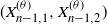
, which comes in terms of
 $(X_{n-1,1}^{(\theta)}, X_{n-1,2}^{(\theta)})$
. So an iterated expectation on each conditional recurrence gives us three unconditional recurrence equations in
 ${\mathbb E}\bigl[(X_{n,1}^{(\theta)})^2\bigr]$
,
 ${\mathbb E}\bigl[X_{n,1}^{(\theta)}X_{n,2}^{(\theta)}\bigr]$
, and
 ${\mathbb E}\bigl[(X_{n,2}^{(\theta)})^2\bigr]$
.
It is evident that we need a bootstrapping technique. The recurrence equation for
 ${\mathbb E}\bigl[(X_{n,1}^{(\theta)})^2\bigr]$
is self-contained, going back only to
 ${\mathbb E}\bigl[(X_{n-1,1}^{(\theta)})^2\bigr]$
, so we can start there. It has the form (14), with solution
 \begin{equation*}{\mathbb E}\bigl[\bigl(X_{n,1}^{(\theta)}\bigr)^2\bigr] = \dfrac {n^2}{\theta^2} +\dfrac {5\theta^2-4\theta+1}{\theta^2(2\theta-1)}\, n + {\mathrm{O}} (1).\end{equation*}
The recurrence equation for
 ${\mathbb E}\bigl[X_{n,1} ^{(\theta)} X_{n,2} ^{(\theta)}\bigr]$
involves
 ${\mathbb E}\bigl[\bigl(X_{n-1,1}^{(\theta)}\bigr)^2\bigr]$
, which is now available. So, after all, the equation is of the form (14) (with some of the terms in
 $h_n$
specified only asymptotically). We obtain the asymptotic solution
 \begin{equation*}{\mathbb E}\bigl[X_{n,1} ^{(\theta)} X_{n,2}^{(\theta)}\bigr] = \dfrac {\theta -1}{\theta^2}\, n^2 + \dfrac {7\theta^4-16\theta^3+14 \theta^2 -6\theta +1}{\theta^3(2\theta-1)^2}\, n + {\mathrm{O}} (\!\ln (n)).\end{equation*}
Similarly, the recurrence equation for
 ${\mathbb E}\bigl[(X_{n,2}^{(\theta)})^2\bigr]$
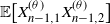
involves
 ${\mathbb E}\bigl[(X_{n-1,1}^{(\theta)})^2\bigr]$
and
 ${\mathbb E}\bigl[X_{n-1,1}^{(\theta)}X_{n-1,2}^{(\theta)}\bigr]$
, which are both available now. Again, the equation is of the form (14) (with
 $h_n$
specified only asymptotically). This gives the solution
 \begin{equation*}{\mathbb E}\bigl[(X_{n,2}^{(\theta)})^2\bigr] = \dfrac {(\theta -1)^2}{\theta^4}\,n^2 + \dfrac {(22\theta^4-30\theta^3 + 20 \theta^2 -7\theta +1)(\theta-1)^2}{\theta^4(2\theta-1)^3}\,n +{\mathrm{O}} (\!\ln (n)).\end{equation*}
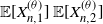
For the variance, from the second moments we subtract the expectations of the squares of the first moments, and for the covariance, we subtract
 ${\mathbb E}[X_{n,1}^{(\theta)}]\, {\mathbb E}[X_{n,2}^{(\theta)}]$
from the mixed moment. Huge cancelations take place, removing the
 $n^2$
-term from the expression and leaving the covariance matrix convergence as stated. A reader interested in checking out all the details can find them in the extended arXiv version [Reference Sparks, Balaji and Mahmoud16].
5.3. Concentration laws
We determine approximations of
 $X_{n,1}^{(\theta)}$
and
 $X_{n,2}^{(\theta)}$
by the leading asymptotic equivalents of their means. A sequence of random variables
 $Y_n$
is
 ${\mathrm{O}}_{{\mathcal{L}}_1} (g(n))$
when there exist a positive constant A and a positive integer
 $n_0$
, such that
 ${\mathbb E}[|Y_n|] \le A |g(n)|$
for all
 $n \ge n_0$
. Errors in the
 ${\mathrm{O}}_{{\mathcal{L}}_1}$
sense are of lower order.
Lemma 3. As
 $n\to\infty$
, we have the asymptotic approximation
 \begin{equation*}\begin{pmatrix} X_{n,1}^{(\theta)}\\[8pt] X_{n,2}^{(\theta)} \end{pmatrix} = \begin{pmatrix}\displaystyle \dfrac n \theta + {\mathrm{O}}_{{\mathcal{L}}_1} (\sqrt n)\\[12pt] \displaystyle \dfrac {(\theta-1) n} {\theta^2} + {\mathrm{O}}_{{\mathcal{L}}_1} (\sqrt n ) \end{pmatrix}\!.\end{equation*}
Proof. From the asymptotics of the mean and variance, as given in Proposition 2 and Theorem 4, we have
 \begin{align*} {\mathbb E}\biggl[\biggl(X_{n,1}^{(\theta)} - \dfrac n \theta \biggr)^2\biggr] &= {\mathbb E}\biggl[\biggl(\bigl(X_{n,1}^{(\theta)} - {\mathbb E}\bigl[X_{n,1}^{(\theta)}\bigr]\bigr) + \biggl({\mathbb E}\bigl[X_{n,1}^{(\theta)}\bigr] - \dfrac n \theta\biggr)\biggr) ^2\biggr]\\ &=\operatorname{Var}\bigl[X_{n,1}^{(\theta)}\bigr] + \biggl({\mathbb E}\bigl[X_{n,1}^{(\theta)}\bigr] -\dfrac n \theta \biggr)^2\\ &= {\mathrm{O}} (n). \end{align*}
So, by Jensen’s inequality
 \begin{equation*}{\mathbb E}\biggl[\biggl| X_{n,1}^{(\theta)} - \dfrac n \theta \biggr|\biggr] \le \sqrt {{\mathbb E}\biggl[\biggl(X_{n,1}^{(\theta)}- \dfrac n \theta \biggr)^2\biggr] } = {\mathrm{O}} (\sqrt n).\end{equation*}
It follows that
 \begin{equation*}X_{n,1}^{(\theta)} = \dfrac n \theta + {\mathrm{O}}_{{\mathcal{L}}_1} (\sqrt n).\end{equation*}
The proof of the asymptotic approximation for
 $X_{n,2}^{(\theta)}$
is quite similar.
5.4. Martingalization
We perform a martingale transform on
 $X_{n,1}^{(\theta)}$
. Let
 $M_n^{(\theta)} = r_n^{(\theta)} X_{n,1}^{(\theta)}+ s_n^{(\theta)}$
, for deterministic – but yet-to-be specified – factors
 $r_n^{(\theta)}$
and
 $s_n^{(\theta)}$
that render
 $M_n^{(\theta)}$
a martingale. For such martingalization, using (11), we write
 \begin{align*}{\mathbb E}\bigl[M_n^{(\theta)}\mid {\mathbb F}^{(\theta)}_{n-1}\bigr] &= {\mathbb E}\bigl[r_n^{(\theta)} X_{n,1}^{(\theta)} + s_n^{(\theta)}\mid {\mathbb F}^{(\theta)}_{n-1}\bigr] \\ &= \biggl(1-\dfrac{\theta-1}{\tau_{n-1}^{(\theta)}}\biggr) r_n ^{(\theta)} X_{n-1,1}^{(\theta)}+r_n ^{(\theta)}+ s_n ^{(\theta)}\\ &= M_{n-1}^{(\theta)}\\ &= r_{n-1}^{(\theta)} X_{n-1,1}^{(\theta)} + s_{n-1}^{(\theta)}.\end{align*}
This is possible if
 \begin{align*} r_{n-1}^{(\theta)} &= \biggl(1 - \dfrac{\theta-1} {\tau_{n-1}^{(\theta)}}\biggr) r_n^{(\theta)}, \\ s_{n-1} ^{(\theta)}&= r_n^{(\theta)} + s_n^{(\theta)}.\end{align*}
The factor
 $r_n^{(\theta)}$
should satisfy the recurrence
 \begin{equation*} r_n^{(\theta)} = \biggl(\dfrac {\tau_{n-1}^{(\theta)}} {\tau_{n-1}^{(\theta)} -\theta+1} \biggr) r_{n-1} = \biggl(\dfrac {n+\theta-1} n \biggr)r_{n-1}^{(\theta)} , \end{equation*}
which unwinds into
 \begin{equation*} r_n^{(\theta)} = \dfrac {(n+\theta-1) (n+\theta-2) \cdots \theta}{n(n-1)\times \cdots \times 1}\, r_0^{(\theta)} = \dfrac {\Gamma(n+\theta)} {\Gamma (\theta)\, \Gamma(n+1)}\, r_0^{(\theta)} \end{equation*}
for any arbitrary
 $r_0^{(\theta)}\in \mathbb R$
; for simplicity, we take
 $r_0^{(\theta)} =1$
.
The factor
 $s_n^{(\theta)}$
should satisfy the recurrence
 \begin{equation*}s_n^{(\theta)} = s_{n-1}^{(\theta)} - r_{n}^{(\theta)} ,\end{equation*}
which unwinds into
 \begin{equation*}s_n^{(\theta)} = s_0^{(\theta)}- \sum_{i=1}^{n} r_i^{(\theta)}\end{equation*}
for any arbitrary
 $s_0^{(\theta)} \in \mathbb R$
; we take
 $s_0^{(\theta)} = 0$
. Using the identity (15) once again, we simplify
 $s_n^{(\theta)}$
to
 \begin{equation*}s_n^{(\theta)} = - \dfrac { \Gamma(n+\theta+1)}{\theta\, \Gamma(\theta)\,\Gamma(n+1) } +1.\end{equation*}
Thus we deduce that
 \begin{equation*} M_n^{(\theta)} = \dfrac {\Gamma(n+\theta)} {\Gamma (\theta)\, \Gamma(n+1)} \, X_{n,1}^{(\theta)} - \dfrac {\Gamma(n+\theta+1)}{\theta\,\Gamma(\theta)\,\Gamma(n+1)} + 1\end{equation*}
is a martingale.
Asymptotics of
 $r_n^{(\theta)}$
,
 $s_n^{(\theta)}$
and their backward differences are useful in the ensuing analysis.
Lemma 4. As
 $n\to\infty$
, we have the asymptotics
 \begin{equation*} r_n^{(\theta)} \sim \dfrac {n^{\theta-1}} {\Gamma (\theta)}, \quad r_n^{(\theta)}-r_{n-1}^{(\theta)} = {\mathrm{O}} (n^{\theta-2}),\end{equation*}
 \begin{equation*} s_n^{(\theta)} \sim - \dfrac {n^\theta} {\theta \, \Gamma(\theta)}, \quad s_n^{(\theta)}-s_{n-1}^{(\theta)} = {\mathrm{O}} (n^{\theta-1}).\end{equation*}
Proof. Examine the forms of
 $r_n^{(\theta)}$
and
 $s_n^{(\theta)}$
. Their asymptotic equivalents follow from the Stirling approximation in (5).
Further, we have
 \begin{align*}r_n^{(\theta)} - r_{n-1}^{(\theta)} &= \dfrac {\Gamma(n+\theta)} {\Gamma (\theta)\, \Gamma(n+1)} - \dfrac {\Gamma(n-1+\theta)} {\Gamma (\theta)\, \Gamma(n)} \\[4pt] &= \dfrac {\Gamma(n-1+\theta)} {\Gamma (\theta)\, \Gamma(n)} \biggl(\dfrac{n-1+\theta} n -1\biggr)\\[4pt] &\sim \dfrac{\theta-1} {\Gamma (\theta)} \,n^{\theta-2} \end{align*}
and
 \begin{align*}s_n^{(\theta)} - s_{n-1}^{(\theta)} &= - \dfrac {\Gamma(n+\theta+1)} {\theta\,\Gamma(\theta)\,\Gamma(n+1)} + \dfrac { \Gamma(n+\theta)} {\theta \,\Gamma(\theta)\,\Gamma(n)} \\[4pt] &= -\dfrac {\Gamma(n+\theta)} {\theta\,\Gamma(\theta)\, \Gamma(n)} \biggl(\dfrac{n+\theta} {n} -1\biggr)\\[4pt] &= -\dfrac {\Gamma(n+\theta)} {\Gamma(\theta)\, \Gamma(n+1)}\\[4pt] &\sim \dfrac {n^{\theta-1}}{\Gamma(\theta)}. \end{align*}
Corollary 1. For large enough positive constants
 $K_1, K_2$
, and
 $K_3$
, we have
 \begin{equation*} r_n^{(\theta)} \le K_1 n^{\theta-1}, \quad r_n^{(\theta)}-r_{n-1}^{(\theta)} \le K_2 n^{\theta-2},\quad s_n^{(\theta)}-s_{n-1}^{(\theta)} = K_3n^{\theta-1}\end{equation*}
for all
 $n\ge 1$
.
5.5. Gaussian limit law
In this subsection we obtain an asymptotic Gaussian law for
 $X_{n,1}^{(\theta)}$
by verifying the conditions of the martingale central limit theorem for
 $M_n^{(\theta)}$
. We use the conditional Lindeberg condition and the conditional variance condition in [Reference Hall and Heyde6, pages 57–59].
The conditional Lindeberg condition requires that for some positive sequence
 $\xi_n^{(\theta)}$
and for any
 $\varepsilon>0$
we have
 \begin{equation*} U_n^{(\theta)} \,:\!=\, \sum_{j = 1}^{n}{\mathbb E} \biggl[ \biggl( \dfrac{\nabla M_j^{(\theta)}}{\xi_n^{(\theta)}} \biggr)^2 {\mathbb I}_ {\{|{{{\nabla M_j^{(\theta)}}}/{{\xi_n^{(\theta)}}}} | > \varepsilon\}} \Bigm| {\mathbb F}^{(\theta)}_{j - 1} \biggr] \buildrel {\mathcal{P}} \over \longrightarrow 0,\end{equation*}
and the conditional variance condition requires that, for some random variable
 $G_\theta \not \equiv 0$
, we have
 \begin{equation*}V_n^{(\theta)}\,:\!=\, \sum_{j = 1}^{n} {\mathbb E} \biggl[ \biggl( \dfrac{\nabla M_j^{(\theta)}}{\xi_n^{(\theta)}} \biggr)^2 \Bigm| {\mathbb F}^{(\theta)}_{j - 1} \biggr] \buildrel {\mathcal{P}} \over \longrightarrow G_\theta.\end{equation*}
When these conditions are satisfied, we get
 \begin{equation*}\dfrac {M_n^{(\theta)}} {\xi_n^{(\theta)}} \ {\buildrel {\mathcal{D}} \over \longrightarrow}\ {\mathcal{N}} (0, G_\theta),\end{equation*}
where the right-hand side is a mixture of normally distributed random variates, with mixing variance
 $G_\theta$
. In our case we find that
 $G_\theta$
is a constant, so the mixture has only one normal random variate in it, which has a deterministic variance. In the case of the number of vertices at containment level 1, it turns out that
 $\xi_n^{(\theta)}$
is
 $n^{\theta - {{1}/{2}}}$
.
The following uniform bound paves the way to the verification of the two conditions of the martingale central limit theorem.
Lemma 5. The absolute differences
 $|\nabla M_j^{(\theta)}|/ n^{\theta - 1}$
are uniformly bounded in
 $j = 1, \ldots, n$
.
Proof. By the construction of the martingale, for each
 $ 1 \le j \le n $
, we have
 \begin{align*}\bigl|\nabla M_j^{(\theta)}\bigr| &= \bigl|M_j^{(\theta)} - M_{j - 1}^{(\theta)}\bigr|\\[4pt] &= \bigl|\bigl(r_j^{(\theta)} X_{j,1}^{(\theta)} + s_j^{(\theta)}\bigr) - \bigl(r_{j - 1}^{(\theta)}X_{j-1,1}^{(\theta)} + s_{j - 1}^{(\theta)}\bigr)\bigr| \\[4pt] & \le \bigl|r_j^{(\theta)} \bigl(X_{j-1,1}^{(\theta)} - Q_{j,1}^{(\theta)} +1\bigr) - r_{j - 1}X_{j-1,1}^{(\theta)}\bigr| + \bigl| s_j^{(\theta)} - s_{j - 1}^{(\theta)}\bigr|\\[4pt] &\le \bigl|r_j^{(\theta)} -r_{j-1}^{(\theta)}\bigr|\, \tau_{j-1}^{(\theta)} + r_j ^{(\theta)} Q_{j,1}^{(\theta)} + r_j^{(\theta)} + \bigl| s_j^{(\theta)} - s_{j - 1}^{(\theta)}\bigr|. \end{align*}
Recall that
 $Q_{n,1}^{(\theta)}$
is a hypergeometric random variable representing the number of vertices at containment level 1 in a sample of size
 $\theta -1$
. Its maximum value is
 $\theta-1$
.
From the bounds in Corollary 1, we obtain
 \begin{align*} \biggl|\dfrac{\nabla M_j^{(\theta)}} {n^{\theta -1}}\biggr| &\le \dfrac 1 {n^{\theta - 1}} \bigl(K_2j^{\theta-2} \, \tau_{n-1}^{(\theta)} + (\theta-1) K_1 j^{\theta-1} + K_1 j^{\theta-1} + K_3n^{\theta -1} \bigr) \\ &\le \dfrac 1 {n^{\theta - 1}} \bigl(K_2n^{\theta-2} (n+\theta -1) + \theta K_1 n^{\theta -1} \bigr) + K_3\\ &= K_2 + \dfrac {(\theta-1)K_2}n+ \theta K_1 +K_3\\ & \le K_2 +(\theta-1)K_2+ \theta K_1 +K_3. \end{align*}
Lemma 6. For any
 $\varepsilon > 0$
, we have
 \begin{align*} U_n^{(\theta)} = \sum_{j = 1}^n {\mathbb E} \biggl[ \biggl( \dfrac{\nabla M_j^{(\theta)}} {n^{\theta - {{1}/{2}}}} \biggr)^2 {\mathbb I}_{\{|{{{\nabla M_j^{(\theta)}}}/{{n^{\theta-1/ 2 }}}} | > \varepsilon\}} \Bigm| {\mathbb F}^{(\theta)}_{j - 1} \biggr] \buildrel {\mathcal{P}} \over \longrightarrow 0. \end{align*}
Proof. By the uniform bound established in Lemma 5, for every
 $\varepsilon>0$
, there exists a natural number
 $n_0 (\varepsilon) $
, such that for all
 $ n \ge n_0 (\varepsilon)$
, the sets
 $\{|\nabla M_j^{(\theta)} | > \varepsilon {n^{\theta-{{1}/{2}}}} \}$
are empty, which implies that the sequence
 $U_n$
converges almost surely to 0. This almost-sure convergence is stronger than the required in-probability convergence.
Lemma 7.
 \begin{align*} V_n^{(\theta)} = \sum_{j = 1}^{n} {\mathbb E} \biggl[ \biggl( \dfrac{\nabla M_j^{(\theta)}}{n^{\theta -{{1}/{2}}}} \biggr)^2 \Bigm| {\mathbb F}^{(\theta)}_{j - 1} \biggr] \buildrel {\mathcal{P}} \over \longrightarrow \dfrac{\theta-1}{\theta^2(2\theta-1)\, \Gamma^2(\theta)} . \end{align*}
Proof. This is a rather lengthy calculation, but for the large part it goes in the same vein as the computations we encountered in the proof of Theorem 4. So we only outline the salient features in the long chain of calculations.
Write
 \begin{align*} V_n^{(\theta)} &= \dfrac{1}{n^{2\theta-1}}\sum_{j = 1}^{n} {\mathbb E} \bigl[\bigl(\nabla \bigl(r_j^{(\theta)} X_{j,1}^{(\theta)}\bigr) + \nabla s_j^{(\theta)}\bigr)^2\bigr] \mid {\mathbb F}^{(\theta)}_{j - 1} \bigr]\\ &= \dfrac{1}{n^{2\theta-1}} \sum_{j = 1}^{n} {\mathbb E} \bigl[\bigl(\nabla \bigl(r_j^{(\theta)} X_{j,1}^{(\theta)}\bigr)\bigr)^2 + 2 \bigl(\nabla \bigl(r_j^{(\theta)} X_{j,1}^{(\theta)}\bigr)\bigr) \nabla s_j^{(\theta)} + \bigl(\nabla s_j^{(\theta)}\bigr)^2 \mid {\mathbb F}^{(\theta)}_{j - 1} \bigr]\\ & :\!= \dfrac{1}{n^{2\theta-1}} \sum_{j = 1}^{n} \bigl(A_j^{(\theta)} + B_j^{(\theta)} + D_j^{(\theta)}\bigr). \end{align*}
We take up each part separately, starting with
 \begin{align*} A_j^{(\theta)} & \,:\!=\, {\mathbb E} \bigl[\bigl(\nabla \bigl(r_j^{(\theta)} X_{j,1}^{(\theta)}\bigr)\bigr)^2 \mid {\mathbb F}^{(\theta)}_{j - 1} \bigr] \\[4pt] &= {\mathbb E} \bigl[\bigl(r_j^{(\theta)} X_{j,1}^{(\theta)} - r_{j-1}^{(\theta)} X_{j-1,1}^{(\theta)}\bigr)^2 \mid {\mathbb F}^{(\theta)}_{j - 1} \bigr]\\[4pt] &= \bigl(r_j^{(\theta)}\bigr)^2\, {\mathbb E}\bigl[\bigl(X_{j,1}^{(\theta)}\bigr)^2 \mid {\mathbb F}^{(\theta)}_{j - 1}\bigr] + \bigl(r_{j - 1}^{(\theta)}\bigr)^2 \bigl(X_{j-1,1}^{(\theta)}\bigr)^2\\[4pt] &\quad\, - 2 r_j^{(\theta)} r_{j - 1}^{(\theta)} X_{j-1,1}^{(\theta)} \, {\mathbb E}\bigl[X_{j,1}^{(\theta)} \mid {\mathbb F}^{(\theta)}_{j - 1}\bigr]\\[4pt] &= \bigl(r_j^{(\theta)}\bigr)^2\, {\mathbb E}\bigl[\bigl(X_{j-1,1}^{(\theta)} - Q_{j,1}^{(\theta)} +1\bigr)^2 \mid {\mathbb F}^{(\theta)}_{j - 1}\bigr] +\bigl( r_{j - 1}^{(\theta)}\bigr)^2 \bigl(X_{j-1,1}^{(\theta)}\bigr)^2\\[4pt] & \quad\, - 2 r_j^{(\theta)} r_{j - 1} ^{(\theta)} X_{j-1,1}^{(\theta)} \, {\mathbb E}\bigl[X_{j-1,1}^{(\theta)} - Q_{j,1}^{(\theta)} +1 \mid {\mathbb F}^{(\theta)}_{j - 1}\bigr] , \end{align*}
where we substituted the right-hand side of (9) for
 $X_{j,1}^{(\theta)}$
. Upon expanding, we get conditional expectations (given
 ${\mathbb F}^{(\theta)}_{j-1}$
) of both
 $(Q_{j,1}^{(\theta)})^2$
and
 $Q_{j,1}^{(\theta)}$
. The variable
 $Q_{j,1}^{(\theta)}$
is
 \begin{equation*}\operatorname{Hypergeo} \bigl(\tau_{j-1}^{(\theta)}, X_{j-1,1}^{(\theta)}, \theta-1\bigr).\end{equation*}
The required conditional expectations are obtained from the hypergeometric distribution; see Section 3. The second part is
 \begin{align*}B_j ^{(\theta)} &= {\mathbb E} \bigl[2 \bigl(\nabla \bigl(r_j^{(\theta)} X_{j,1}^{(\theta)}\bigr)\bigr) \nabla s_j^{(\theta)} \mid {\mathbb F}^{(\theta)}_{j - 1} \bigr]\\ &= 2\, {\mathbb E} \bigl[ \bigl(r_j^{(\theta)} X_{j,1}^{(\theta)} - r_{j-1}^{(\theta)} X_{j-1,1}^{(\theta)}\bigr) \bigl(s_j^{(\theta)}-s_{j-1}^{(\theta)}\bigr) \mid {\mathbb F}^{(\theta)}_{j - 1} \bigr]\\ &= 2\, r_j^{(\theta)} \bigl(s_j^{(\theta)} - s_{j-1}^{(\theta)}\bigr) \, {\mathbb E}\bigl[X_{j,1}^{(\theta)} \mid {\mathbb F}^{(\theta)}_{j-1}\bigr] - 2 r_{j-1}^{(\theta)} \bigl(s_j^{(\theta)}-s_{j-1}^{(\theta)}\bigr) X_{j-1,1}^{(\theta)}. \end{align*}
The third part is
 \begin{equation*}D_j^{(\theta)} = {\mathbb E} \bigl[\bigl(\nabla s_j^{(\theta)}\bigr)^2 \mid {\mathbb F}^{(\theta)}_{j - 1} \bigr] = \bigl(s_j^{(\theta)}-s_{j-1}^{(\theta)}\bigr)^2.\end{equation*}
We now put the three parts together and get an expression for
 $V_n^{(\theta)}$
as a sum, in which the summand is in terms of
 $r_j^{(\theta)}$
and
 $s_j^{(\theta)}$
, and their backward differences, as well as
 $X_{j-1,1}^{(\theta)}$
. For simplified asymptotics, we use the asymptotic equivalents in Lemma 3 for
 $X_{j-1, 1}^{(\theta)}$
, and for
 $r_j^{(\theta)}$
,
 $s_j^{(\theta)}$
,
 $\nabla r_j^{(\theta)}$
,
 $\nabla s_j^{(\theta)}$
, we use the asymptotics in Lemma 4.
Huge cancelations take place, leaving
 \begin{align*} V_{n}^{(\theta)} &= \dfrac 1 {n^{2\theta - 1}} \biggl( \sum_{j=1}^n \dfrac{(\theta-1)^2}{\theta^2\, \Gamma^2(\theta)} j^{2\theta-2} + {\mathrm{O}}_{{\mathcal{L}}_1}(j^{2\theta-3})\biggr)\\ &= \dfrac{(\theta-1)^2}{\theta^2(2\theta-1)\, \Gamma^2(\theta)} + {\mathrm{O}}_{{\mathcal{L}}_1}\biggl(\dfrac 1 n\biggr)\\ &\buildrel {{\mathcal{L}}_1} \over \longrightarrow \dfrac{(\theta-1)^2}{\theta^2(2\theta-1)\, \Gamma^2(\theta)}. \end{align*}
This
 ${\mathcal{L}}_1$
convergence is stronger than the required in-probability convergence.
Theorem 5. Let
 $X_{n,1}^{(\theta)}$
be the number of vertices in hyper-recursive tree with hyperedges of size
 $\theta$
at age n. Then, as
 $n\to\infty$
, we have
 \begin{equation*}\dfrac {X_{n,1}^{(\theta)} - {{n}/{\theta}} } {\sqrt n}\ {\buildrel {\mathcal{D}} \over \longrightarrow}\ {\mathcal{N}} \biggl(0, \dfrac{(\theta-1)^2}{\theta^2(2\theta-1)} \biggr).\end{equation*}
Proof. Having checked the conditions for the martingale central limit theorem, we can ascertain that
 \begin{align*}\dfrac {M_n^{\theta}} {n^{\theta - {{1}/{2}}}} &=\dfrac { \frac {\Gamma(n+\theta)} {\Gamma (\theta)\, \Gamma(n+1)} \, X_{n,1}^{(\theta)} - \frac {\Gamma(n+\theta+1) }{\theta\,\Gamma(\theta)\,\Gamma(n+1)}+1} {n^{\theta - {{1}/{2}}}} \\[4pt]&= \dfrac { \frac {\Gamma(n+\theta)} {\Gamma (\theta)\, \Gamma(n+1)} \, X_{n,1}^{(\theta)} - \frac {\Gamma(n+\theta)} {\Gamma(\theta) \, \Gamma(n+1)}\bigl(\frac{n}{\theta}\bigr)- \frac {\Gamma(n+\theta) }{\Gamma(\theta)\,\Gamma(n+1))}+1} {n^{\theta - {{1}/{2}}}} \\[4pt] & {\buildrel {\mathcal{D}} \over \longrightarrow}\ {\mathcal{N}} \biggl(0, \dfrac{(\theta-1)^2}{\theta^2(2\theta-1)\, \Gamma^2(\theta)} \biggr).\end{align*}
We have
 \begin{equation*}\biggl(- \dfrac {\Gamma(n+\theta) }{\,\Gamma(n+1)\Gamma(\theta)}+1\biggr) ( n^{{{1}/{2}} -\theta } )\to 0,\end{equation*}
and so an application of Slutsky’s theorem [Reference Slutsky14] allows us to remove this term. By the Stirling approximation in (5), we have
 \begin{equation*} \dfrac {n^{\theta-1}\Gamma(n+1)} {\Gamma(n+\theta)}\to 1.\end{equation*}
An application of Slutsky’s theorem [Reference Slutsky14] yields
 \begin{equation*}\dfrac { \frac 1 {\Gamma (\theta)} \,( X_{n,1}^{(\theta)} - \frac n \theta)} {\sqrt n} {\buildrel {\mathcal{D}} \over \longrightarrow}\ N \biggl(0, \dfrac{(\theta-1)^2} {\theta^2(2\theta-1)\, \Gamma^2(\theta)} \biggr),\end{equation*}
which is an equivalent statement to the one given in the theorem.
Remark 4. In the very special case
 $\theta=2$
, the hyper-recursive tree is the standard uniform recursive tree. In this case
 $X_{n,1}^{(2)}$
is just a count of the leaves in the tree. Theorem 5 recovers the result in [Reference Mahmoud and Smythe12] and generalizes it.
Acknowledgements
We wish to thank the referees for suggesting a redirection of the proof that led to a finer presentation.
Funding information
There are no funding bodies to thank relating to this creation of this article.
Competing interests
There were no competing interests to declare which arose during the preparation or publication process of this article.