Nomenclature

LCO

limit cycle oscillation

SDRE

state-dependent Riccati equation

DoF

degree of freedom

AFS

active flutter suppression

a

non-dimensional distance from wing mid- chord to elastic axis

b

wing semi-chord

c

non-dimensional distance from wing mid- chord to the control surface hinge line

disp.

displacement

def.

deflection

$ {c}_{i}$

Wagner function coefficients, i = 0, 1, 2, 3, 4

h

plunge displacement

$ {c}_{{\mathrm{k}}_{\mathrm{\alpha }}}$

reduced stiffness coefficient

$ {I}_{\alpha }$

mass moment of inertia of wing-flap about a

$ {I}_{\beta }$

mass moment of inertia of flap about c

$ {k}_{h}$

stiffness in deflection

$ {k}_{\beta }$

stiffness in flap rotation

l

wing span

L

lift force

M

aerodynamic pitching moment about elastic axis

$ {m}_{a}$

mass of flap

m

total mass of wing-flap (per unit span)

$ {m}_{sup}$

mass of support blocks

$ {m}_{t}$

total mass of wing-flap and support blocks (per unit span)

$ {m}_{w}$

mass of wing

$ {r}_{\alpha }$

reduced radius of gyration of the wing-flap divided by b

$ {r}_{\beta }$

reduced radius of gyration of the flap divided by b

T

aerodynamic hinge moment about flap hinge line

$ {x}_{\alpha }$

non-dimensional distance from wing elastic axis to centre of mass

$ {x}_{\beta }$

non-dimensional distance from flap hinge line to centre of mass

$ {G}_{\alpha}\!\left(\alpha \right)$

cubic nonlinear function to represent the nonlinear torsional stiffness effects

Greek symbol

α

pitch about elastic axis

β

flap deflection about the hinge axis

β_c

commanded deflection or control input

$ \gamma $

nonlinear parameter in pitch stiffness

$ \delta $

total angular size of the freeplay region

$ {\rho }_{a}$

air density

$ {\zeta }_{1}$

modal damping ratio of plunge

$ {\zeta }_{2}$

modal damping ratio of pitch

$ {\zeta }_{3}$

modal damping ratio of flap

2.0 Mathematical modeling of an aeroelastic wing

A three DoF wing section elastically supported by a linear plunge spring and a nonlinear torsional spring is illustrated in Fig. 1. This wing section is equipped with a control surface which is constrained with another nonlinear torsional spring. Three DoF of the wing and flap are modeled with three springs, one compression spring (for plunging motion and stiffness in deflection) and two torsional springs (for stiffness in pitch and flap rotation).

Figure 1.

Aeroelastic model with freeplay nonlinearity in the control surface.

The nonlinearity associated with the control surface – due to worn hinge or loose attachments – is called freeplay [Reference Dhital and Han6]. It means that spring stiffness will be a nonlinear function of angle of torsion. Hence, torsional spring (connection of the control surface to the wing) cannot carry forces for some angles of control surface’s displacement [Reference Jafari, Feizarefi and Majidi Pishkenari11]. The freeplay nonlinearity in the aeroelastic system is modeled using a set of linear piecewise functions, which is represented by $ {G}_{\beta}(\beta)$ . The piecewise restoring torque for the flap motions is defined as:

(1) \begin{align} {k}_{\beta }{G}_{\beta}\!\left(\beta \right)=\left\{\begin{array}{c}\begin{array}{c@{\quad}c}{k}_{\beta }\left(\beta -\delta \right),& \beta \gt \delta ,\end{array}\\[5pt] \begin{array}{c@{\quad}c}0, &-\delta \le \beta \end{array}\le \delta ,\\[5pt] \begin{array}{c@{\quad}c}{k}_{\beta }\left(\beta +\delta \right), &\beta \leftarrow \delta \end{array}\end{array}\right.\end{align}

The model is permitted to have three freedoms: to plunge, h; to pitch, α about an elastic axis; and flap deflection β about the hinge axis. The non-dimensional form of governing equations [Reference Li, Guo and Xiang13] for structural dynamics of wing section with control surface is given as:

(2) \begin{align}\begin{cases}\displaystyle \hspace{54pt}{{{{m_t}} \over {mb}}\ddot h + {x_\alpha }\ddot \alpha + {x_\beta }\ddot \beta + {{{k_h}} \over {mb}}{G_h}\left( h \right) = {L \over {mb}}} \\[12pt] \displaystyle {{{{x_\alpha }} \over b}\ddot h + {{{I_\alpha }} \over {m{b^2}}}\ddot \alpha + {c_{{k_\alpha }}}{{{k_\alpha }} \over {m{b^2}}}{G_\alpha }\left( \alpha \right) + \left[ {{{{I_\beta }} \over {m{b^2}}} + \left( {c - a} \right){x_\beta }} \right]\ddot \beta = {M \over {m{b^2}}}} \\[12pt] \displaystyle {\left[ {{{{I_\beta }} \over {m{b^2}}} + \left( {c - a} \right){x_\beta }} \right]\ddot \alpha + {{{x_\beta }} \over b}\ddot h + {{{I_\beta }} \over {m{b^2}}}\ddot \beta + {{{k_\beta }} \over {m{b^2}}}\left( {{G_\beta }\left( \beta \right) - {\beta _c}} \right) = {T \over {m{b^2}}}} \end{cases} \end{align}

In this paper, the existence of damage on the wing section is dynamically modeled through its effects. That is, the damage is modeled with using a stiffness reduction coefficient on the cubic nonlinear pitch spring. The $ {c}_{{k}_{\alpha }}$ denotes reduced stiffness coefficient; when $ {c}_{{k}_{\alpha }}$ is equal to one, it means there is no damage. By defining new variables and assuming that plunge stiffness is linear and considering a cubic nonlinear spring in pitch, the following new parameters are introduced:

(3) \begin{align} \mathrm{\xi }=\frac{h}{b},{\omega }_{\xi }=\sqrt{\frac{{k}_{\xi }}{m}},{G}_{h}\left(h\right)=h,\frac{{I}_{\alpha }}{m{b}^{2}}={{r}_{\alpha }}^{2},\frac{{k}_{\alpha }}{m{b}^{2}}={{\omega }_{\alpha }}^{2}{{r}_{\alpha }}^{2},\frac{{I}_{\beta }}{m{b}^{2}}={{r}_{\beta }}^{2},\frac{{k}_{\beta }}{m{b}^{2}}={{\omega }_{\beta }}^{2}{{r}_{\beta }}^{2},{G}_{\alpha }=\alpha +\gamma {\alpha }^{3}\end{align}

Using new parameters introduced in Equation (3), the Equation (2) may be reformatted as:

(4) \begin{align}\left\{\begin{array}{c}\displaystyle \frac{{m}_{t}}{m}\ddot{\xi }+{x}_{\alpha }\ddot{\alpha }+{x}_{\beta }\ddot{\beta }+{{\omega }_{\xi }}^{2}\xi =\frac{L}{mb}\\[12pt] \displaystyle {x}_{\alpha }\ddot{\xi }+{{r}_{\alpha }}^{2}\ddot{\alpha }+{c}_{{k}_{\alpha }}{{\omega }_{\alpha }}^{2}{{r}_{\alpha }}^{2}\frac{{G}_{\alpha}\!\left(\alpha \right)}{\alpha }\alpha +\left[{{r}_{\beta }}^{2}+\left(c-a\right){x}_{\beta }\right]\ddot{\beta }=\frac{M}{m{b}^{2}}\\[12pt] \displaystyle \left[{{r}_{\beta }}^{2}+\left(c-a\right){x}_{\beta }\right]\ddot{\alpha }+{x}_{\beta }\ddot{\xi }+{{r}_{\beta }}^{2}\ddot{\beta }+{{\omega }_{\beta }}^{2}{{r}_{\beta }}^{2}\frac{\left({G}_{\beta}\!\left(\beta \right)-{\beta }_{c}\right)}{\beta }\beta =\frac{T}{m{b}^{2}}\end{array}\right.\end{align}

Thus, the cubic term related to pitch stiffness ( $ {G}_{\alpha}\!\left(\alpha \right)$ ), is scaled using the scalar parameter ( $ {c}_{{k}_{\alpha }}$ ). This implies that, pitch spring is always nonlinear and its influence on the system, due to existence of damage, is being modified. The matrix form of these equations is obtained as:

(5) \begin{align} {M}_{s}\ddot{\mathit{x}}+{K}_{s}\mathit{x}={F}_{a}\end{align}

where:

(6) \begin{align} {M}_{s}=\left[\begin{array}{c@{\quad}c@{\quad}c}\displaystyle\frac{{m}_{t}}{m}& {x}_{\alpha }& {x}_{\beta }\\[8pt] {x}_{\alpha }& {{r}_{\alpha }}^{2} &\left[{{r}_{\beta }}^{2}+\left(c-a\right){x}_{\beta }\right]\\[8pt] {x}_{\beta}& \left[{{r}_{\beta }}^{2}+\left(c-a\right){x}_{\beta}\right]& {{r}_{\beta }}^{2}\end{array}\right],\mathit{x}=\left\{\begin{array}{c}\xi \\[8pt] \alpha \\[8pt] \beta \end{array}\right\}\end{align}

(7) \begin{align} {K}_{s}=\left[\begin{array}{c@{\quad}c@{\quad}c}\displaystyle{{\omega }_{\xi }}^{2}& 0& 0\\[12pt] 0& {c}_{{k}_{\alpha }}{{\omega }_{\alpha }}^{2}{{r}_{\alpha }}^{2}{G}_{\alpha}\!\left(\alpha \right)/\alpha& 0\\[12pt] 0& 0& {{\omega }_{\beta }}^{2}{{r}_{\beta }}^{2}\left({G}_{\beta}\!\left(\beta \right)-{\beta }_{c}\right)/\beta \end{array}\right],{F}_{a}=\left\{\begin{array}{c}\displaystyle\frac{L}{mb}\\[12pt] \displaystyle\frac{M}{m{b}^{2}}\\[12pt] \displaystyle\frac{T}{m{b}^{2}}\end{array}\right\}\end{align}

By including structural damping, Equation (5) is modified and represented into this short form:

(8) \begin{align} {M}_{s}\ddot{x}+{B}_{s}\dot{x}+{K}_{s}x={F}_{a}\end{align}

The parameter $ {B}_{s}$ is the structural damping matrix and is defined by Liu & Dowell [Reference Liu and Dowell14]:

(9) \begin{align} {B}_{s}={\left({\unicode{x1D6EC} }^{T}\right)}^{-1}{B}_{mod}{\left(\unicode{x1D6EC} \right)}^{-1},{B}_{mod}=\left[\begin{array}{c@{\quad}c@{\quad}c}2{m}_{1}{\omega }_{1}{\zeta }_{1}& 0 &0\\[8pt] 0& 2{m}_{2}{\omega }_{2}{\zeta }_{2}& 0\\[8pt] 0& 0& 2{m}_{3}{\omega }_{3}{\zeta }_{3}\end{array}\right]\end{align}

where $ {\zeta }_{i}$ are measured damping ratios, $ {m}_{i}$ denotes modal mass and $ {\omega }_{i}$ represents coupled natural frequencies. To determine modal masses and natural frequencies, first, the eigenvalues $ {\lambda }_{i}$ and eigenvectors $ \mathrm{\Lambda }$ are calculated from the system: $ {M}_{s}\ddot{\mathit{x}}+{K}_{s}\mathit{x}=0$ . Then, $ {\omega }_{i}=\sqrt{{\lambda }_{i}}$ . Finally $ {m}_{i}$ are the values at the diagonal entries of $ {M}_{mod}$ , where ( $ {M}_{mod}={\mathrm{\Lambda }}^{T}{M}_{s}\mathrm{\Lambda }$ ). The lift, pitching moment, and hinge moment are obtained by Liu & Dowell [Reference Liu and Dowell14]:

(10) \begin{align} \begin{aligned}L&=-\rho {b}^{2}\left(\pi U\dot{\alpha }+\pi \ddot{h}-\pi ba\ddot{\alpha }-U{T}_{4}\dot{\beta}-b{T}_{1}\ddot{\beta }\right)\\[5pt]&\quad-2\pi \rho UbC\left(k\right)\left(U\alpha +\dot{h}+b\left(\frac{1}{2}-a\right)\dot{\alpha }+\frac{1}{\pi }{T}_{10}U\beta +\frac{b}{2\pi }{T}_{11}\dot{\beta }\right)\end{aligned}\end{align}

(11) \begin{align}\begin{aligned}T&=-\rho {b}^{2}\left\{\left[-2{T}_{9}-{T}_{1}+{T}_{4}\left(a-\frac{1}{2}\right)\right]Ub\dot{\alpha }+2{T}_{13}{b}^{2}\ddot{\alpha }+\frac{1}{\pi }{U}^{2}\beta \left({T}_{5}-{T}_{4}{T}_{10}\right)-\frac{1}{2\pi }Ub\dot{\beta }{T}_{4}{T}_{11}\right.\\[5pt]&\quad\left.\kern-1pt-\frac{1}{\pi }{T}_{3}{b}^{2}\ddot{\beta }-{T}_{1}b\ddot{h}\right\}-\rho U{b}^{2}{T}_{12}C\left(k\right)\left[U\alpha +\dot{h}+b\left(\frac{1}{2}-a\right)\dot{\alpha }+\frac{1}{\pi }U{T}_{10}\beta +\frac{b}{2\pi }{T}_{11}\dot{\beta }\right]\\[-18pt]\end{aligned}\end{align}

(12) \begin{align}\begin{aligned} M&=-\rho {b}^{2}\left\{\pi \left(\frac{1}{2}-a\right)Ub\dot{\alpha }+\pi {b}^{2}\left(\frac{1}{8}+{a}^{2}\right)\ddot{\alpha }+\left({T}_{4}+{T}_{10}\right){U}^{2}\beta\right. \\[5pt]&\quad\left.\kern-1pt+\left[{T}_{1}-{T}_{8}-\left(c-a\right){T}_{4}+\frac{1}{2}{T}_{11}\right]Ub\dot{\beta }-\left[{T}_{7}+\left(c-a\right){T}_{1}\right]{b}^{2}\ddot{\beta }-a\pi b\ddot{h}\right\}\\[5pt]&\quad+2\rho U{b}^{2}\pi \left(\frac{1}{2}+a\right)C\left(k\right)\left\{U\alpha +\dot{h}+b\left(\frac{1}{2}-a\right)\dot{\alpha }+\frac{1}{\pi }U{T}_{10}\beta +\frac{b}{2\pi }{T}_{11}\dot{\beta }\right\}\end{aligned}\end{align}

$ {T}_{i}$ are Theodorsen constants, $C(k)$ is the generalised Theodorsen function and $ k$ is the reduced frequency of oscillation, $ k=\omega b/U$ . Due to a limit in number of pages, Theodorsen constants are not provided in the paper, but are defined in [Reference Dhital and Han6]. In order to simulate arbitrary motion of the wing, when restricted to simple harmonic motion, the aerodynamic loading associated with Theodorsen’s function in the time domain is replaced by the Duhamel’s formulation as:

(13) \begin{align} {L}_{c}=C\left(k\right)f\!\left(t\right)=f\!\left(0\right)\phi\!\left(\tau \right)+{\int }_{0}^{\tau }\frac{\partial f\!\left(\sigma \right)}{\partial \sigma }\phi\!\left(\tau -\sigma \right)d\sigma \end{align}

where $ \phi\!\left(\tau\right)$ is Wagner function and $ f\!\left(t\right)$ is:

(14) \begin{align} \mathit{f}\!\left(\mathit{t}\right)=\mathit{U}\mathit{\alpha }+\dot{\mathit{h}}+\mathit{b}\left(\frac{1}{2}-\mathit{a}\right)\dot{\mathit{\alpha }}+\frac{1}{\mathit{\pi }}\mathit{U}{\mathit{T}}_{10}\mathit{\beta }+\frac{\mathit{b}}{2\mathit{\pi }}{\mathit{T}}_{11}\dot{\mathit{\beta }}\end{align}

Here, Jones’s approximation is used to simplify the mathematical expression for Theodorsen’s function, while maintaining the physical characteristics as [Reference Liu and Dowell14]:

(15) \begin{align} \mathrm{\phi}\!\left(\mathrm{\tau }\right)\approx {\mathrm{c}}_{0}-{\mathrm{c}}_{1}{\mathrm{e}}^{{-\mathrm{c}}_{2}\mathrm{\tau }}-{\mathrm{c}}_{3}{\mathrm{e}}^{-{\mathrm{c}}_{4}\mathrm{\tau }}\end{align}

Using partial integration technique, Duhamel’s integral is rewritten as:

(16) \begin{align} {L}_{c}=\left({c}_{0}-{c}_{1}-{c}_{3}\right)f\!\left(\tau \right)-{\int^{\tau}_{0}} f\!\left(\sigma \right)\frac{\partial \phi\!\left(\tau -\sigma \right)}{\partial \sigma }d\sigma \end{align}

By introducing an augmented variable $ \stackrel{-}{x}$ , and using the state space method, Equation (16) may be expressed as:

(17) \begin{align} {L}_{c}=\left({c}_{0}-{c}_{1}-{c}_{3}\right)f\!\left(t\right)+{c}_{2}{c}_{4}\left({c}_{1}+{c}_{3}\right)\left(\frac{{U}^{2}}{b}\right)\stackrel{-}{x}+\left({c}_{1}{c}_{2}+{c}_{3}{c}_{4}\right)U\stackrel{\dot{-}}{x}\end{align}

Using Equation (17), the non-dimensional form of aerodynamic force and moments equations are reformatted as:

(18) \begin{align} \begin{aligned}\frac{L}{mb}&=-\frac{\rho b}{m}\left(\pi U\dot{\alpha }+\pi \ddot{h}-\pi ba\ddot{\alpha }-U{T}_{4}\dot{\beta }-b{T}_{1}\ddot{\beta }\right)\\[5pt]&\quad-\frac{2\pi \rho U}{m}\left(\left({c}_{0}-{c}_{1}-{c}_{3}\right)\left(U\alpha +\dot{h}+b\left(\frac{1}{2}-a\right)\dot{\alpha }+\frac{1}{\pi }{T}_{10}U\beta +\frac{b}{2\pi }{T}_{11}\dot{\beta }\right)\right.\\[5pt]&\quad\left.\kern-1pt+{c}_{2}{c}_{4}\left({c}_{1}+{c}_{3}\right)\left(\frac{{U}^{2}}{b}\right)\stackrel{-}{x}+\left({c}_{1}{c}_{2}+{c}_{3}{c}_{4}\right)U\stackrel{\dot{-}}{x}\right)\end{aligned}\end{align}

(19) \begin{align} \begin{aligned}\frac{M}{m{b}^{2}}&=-\frac{\rho }{m}\left\{\pi \left(\frac{1}{2}-a\right)Ub\dot{\alpha }+\pi {b}^{2}\left(\frac{1}{8}+{a}^{2}\right)\ddot{\alpha }+\left({T}_{4}+{T}_{10}\right){U}^{2}\beta\right.\\[5pt] &\quad\left.\kern-1pt+\left[{T}_{1}-{T}_{8}-\left(c-a\right){T}_{4}+\frac{1}{2}{T}_{11}\right]Ub\dot{\beta }-\left[{T}_{7}+\left(c-a\right){T}_{1}\right]{b}^{2}\ddot{\beta }-a\pi b\ddot{h}\right\}+\frac{2\pi \rho U}{m}\left(\frac{1}{2}+a\right)\\[5pt]&\qquad\times \left(\left({c}_{0}-{c}_{1}-{c}_{3}\right)\left(U\alpha +\dot{h}+b\left(\frac{1}{2}-a\right)\dot{\alpha }+\frac{1}{\pi }{T}_{10}U\beta +\frac{b}{2\pi }{T}_{11}\dot{\beta }\right)\right.\\[-2pt]&\qquad\quad\left.+{c}_{2}{c}_{4}\left({c}_{1}+{c}_{3}\right)\left(\frac{{U}^{2}}{b}\right)\stackrel{-}{x}+\left({c}_{1}{c}_{2}+{c}_{3}{c}_{4}\right)U\stackrel{\dot{-}}{x}\right)\\[-18pt]\end{aligned}\end{align}

(20) \begin{align} \begin{aligned}\frac{T}{m{b}^{2}}&=\frac{-\rho }{m}\left\{\left[-2{T}_{9}-{T}_{1}+{T}_{4}\left(a-\frac{1}{2}\right)\right]Ub\dot{\alpha }+2{T}_{13}{b}^{2}\ddot{\alpha }+\frac{1}{\pi }{U}^{2}\left({T}_{5}-{T}_{4}{T}_{10}\right)\beta -\frac{1}{2\pi }Ub\dot{\beta }{T}_{4}{T}_{11}\right.\\[8pt]&\quad\left.\kern-1pt-\frac{1}{\pi }{T}_{3}{b}^{2}\ddot{\beta }-{T}_{1}b\ddot{h}\right\}\\[8pt]&\quad-\frac{\rho U{T}_{12}}{m}\left\{\left({c}_{0}-{c}_{1}-{c}_{3}\right)\left(U\alpha +\dot{h}+b\left(\frac{1}{2}-a\right)\dot{\alpha }+\frac{1}{\pi }U{T}_{10}\beta +\frac{b}{2\pi }{T}_{11}\dot{\beta }\right)\right.\\[8pt]&\quad\left.\kern-1pt+{c}_{2}{c}_{4}\left({c}_{1}+{c}_{3}\right)\left(\frac{{U}^{2}}{b}\right)\stackrel{-}{x}+\left({c}_{1}{c}_{2}+{c}_{3}{c}_{4}\right)U\stackrel{\dot{-}}{x}\right\}\\[-18pt]\end{aligned}\end{align}

By introducing an augmented variable $ \stackrel{-}{x}$ , and using the state space method, the non-dimensional form of aerodynamic force and moments equations are reformatted. By defining vector variables as $ \mathit{x}={\{\begin{array}{c@{\quad}c@{\quad}c}\xi & \alpha & \beta \end{array}\}}^{T}$ and ${\mathit{x}}_{\mathit{a}}={\{\begin{array}{c@{\quad}c}\stackrel{-}{x} {}& \stackrel{\dot{-}}{x}\end{array}\}}^{\mathit{T}}$ and using the matrix form of aeroelastic equations – including structural damping (Equation (9)), we will derive the state space form of aeroelastic equations:

(21) \begin{align} \begin{aligned}\left\{\begin{array}{c}\ddot{\xi }\\[5pt] \ddot{\alpha }\\[5pt] \ddot{\beta }\end{array}\right\}&=-{{M}_{t}}^{-1}{B}_{t}\left\{\begin{array}{c}\dot{\xi }\\[5pt] \dot{\alpha }\\[5pt] \dot{\beta }\end{array}\right\}-{{M}_{t}}^{-1}{K}_{t}\left\{\begin{array}{c}\xi \\[5pt] \alpha \\[5pt] \beta \end{array}\right\}+{{M}_{t}}^{-1}G{\beta }_{c}+{{M}_{t}}^{-1}D\left\{\begin{array}{c}\stackrel{-}{x}\\[5pt] \stackrel{\dot{-}}{x}\end{array}\right\},\\[5pt]&\quad H\mathit{x}=\left[\begin{array}{c@{\quad}c@{\quad}c}0& 0& 0\\[5pt] 0& 0& 0\\[5pt] 0& 0& {{\omega }_{\beta }}^{2}{{r}_{\beta }}^{2}{\beta }_{c}/\beta \end{array}\right]\left\{\begin{array}{c}\xi \\[5pt] \alpha \\[5pt] \beta \end{array}\right\}=\underbrace{\left\{\begin{array}{c}0\\[5pt] 0\\[5pt] {{\omega }_{\beta }}^{2}{{r}_{\beta }}^{2}\end{array}\right\}}_G{\beta }_{c}\end{aligned}\end{align}

The structural and aerodynamic matrices are defined in the appendix. The state space form of the aeroelastic equations is:

(22) \begin{align} \dot{X}=A\!\left(x\right)X+Bu,A\!\left(x\right)=\left[\begin{array}{c@{\quad}c@{\quad}c}{0}_{3\times 3}& {I}_{3\times 3}& {0}_{3\times 2}\\[5pt] -{{M}_{t}}^{-1}{K}_{t}& -{{M}_{t}}^{-1}{B}_{t}& -{{M}_{t}}^{-1}D\\[5pt] {E}_{1}& {E}_{2}& F\end{array}\right],\mathit{B}=\left\{\begin{array}{c}{0}_{3\times 1}\\[5pt] {{M}_{t}}^{-1}G\\[5pt] {0}_{2\times 1}\end{array}\right\}\end{align}

where the state vector $ \mathit{X}$ and its elements are $ \mathit{X}={\{\begin{array}{c@{\quad}c@{\quad}c}\begin{array}{c@{\quad}c}\!\xi & \alpha \end{array} {}& \begin{array}{c@{\quad}c@{\quad}c}\beta & \dot{\xi } {}& \dot{\alpha }\end{array} & {}\begin{array}{c@{\quad}c@{\quad}c}\dot{\beta } {}& \stackrel{-}{x} {}& \stackrel{\dot{-}}{x}\end{array}\end{array}\}}^{T}$ and the control variable is $ u={\beta }_{c}$ , or control surface (here, flap) deflection. It should be noted that the states $ {x}_{7}=\stackrel{-}{x}$ and $ {x}_{8}=\;\stackrel{\dot{-}}{x}$ were augmented variables related to unsteady aerodynamic for describing the effects of wing wake. These states are related to other states using following differential equation [Reference Vasconcellos, Abdelkefi, Marques and Hajj25].

(23) \begin{align}\begin{aligned}\stackrel{\ddot{-}}{x}&=\left\{\!\begin{array}{c@{\quad}c}-{c}_{2}{c}_{4}\left(\dfrac{{U}^{2}}{b}\right) -\left({c}_{2}+{c}_{4}\right)\dfrac{U}{b}\end{array}\!\!\!\!\!\right\}{\mathit{x}}_{\mathit{a}}+\dfrac{1}{b}{S}_{1}\mathit{x}+\dfrac{1}{b}{S}_{2}\dot{\mathit{x}}=\left\{\!\begin{array}{c@{\quad}c}-{c}_{2}{c}_{4}\left(\dfrac{{U}^{2}}{b}\right) -\left({c}_{2}+{c}_{4}\right)\dfrac{U}{b}\end{array}\!\!\!\!\!\right\}\left\{\begin{array}{c}\stackrel{-}{x}\\[5pt] \stackrel{\dot{-}}{x}\end{array}\right\}\\[3pt]&\quad+\dfrac{1}{b}\left\{\!\begin{array}{c@{\quad}c@{\quad}c}0& U& \dfrac{{T}_{10}U}{\pi}\end{array}\!\right\}\left\{\begin{array}{c}\xi \\[5pt] \alpha \\[5pt] \beta \end{array}\right\}+\dfrac{1}{b}\left\{\!\begin{array}{c@{\quad}c@{\quad}c}b& b\left(\dfrac{1}{2}-a\right)& \dfrac{b{T}_{11}}{2\pi}\end{array}\!\right\}\left\{\begin{array}{c}\dot{\xi }\\[5pt] \dot{\alpha }\\[5pt] \dot{\beta }\end{array}\right\}\\[3pt]&=-{c}_{2}{c}_{4}\left(\dfrac{{U}^{2}}{b}\right)\stackrel{-}{x}-\left({c}_{2}+{c}_{4}\right)\dfrac{U}{b}\stackrel{\dot{-}}{x}+\dfrac{U\alpha }{b}+\dfrac{{T}_{10}U}{b\pi }\beta +\dot{\xi }+\left(\dfrac{1}{2}-a\right)\dot{\alpha }+\dfrac{{T}_{11}}{2\pi }\dot{\beta }\end{aligned}\end{align}

Other elements of aerodynamic force and moments and matrices of the state-space model (i.e., constants $ {T}_{i}$ ) are presented in Jafari et al. [Reference Jafari, Feizarefi and Majidi Pishkenari11].

3.0 State-dependent riccati equation for an aeroelastic wing

There are multiple techniques to design a nonlinear controller such as feedback linearisation technique and SDRE. Researchers have examined the stability of the zero dynamics only for the variations in U and a, and revealed that the system is non-minimum phase for a set of values of the U and a. Moreover, for the choice of plunge displacement, an extremely nonlinear zero dynamics is obtained which have multiple equilibrium points and thus, have complex behaviour [Reference Singh and Yim21]. Thus, there is a need to design a control system for the flutter suppression of aeroelastic systems, which may be a non-minimum phase.

The proposed method for controller design of minimum as well as non-minimum phase systems is the SDRE technique. The SDRE technique is a general design method that provides a systematic and effective means of designing nonlinear controllers, observers and filters [Reference Cloutier4]. Moreover, this method provides flexibility in shaping the response characteristics of the pitch angle and as well as the plunge displacement trajectories. To consider an optimal control problem, the performance index for the nonlinear system is defined as:

(24) \begin{align} J=\frac{1}{2}{\int^{\infty }_{0}}\left({X}^{T}Q\!\left(x\right)X+R\!\left(\mathit{x}\right){\beta }_{c}^{2}\right)dt\end{align}

where $ Q\!\left(\mathit{x}\right)$ is a positive definite symmetric matrix and $ R\!\left(\boldsymbol{x}\right)\gt \boldsymbol{0}$ for all $ \boldsymbol{X}$ , and $ J$ must be minimised. The weighting matrix Q and the scalar function R(x) are properly selected for obtaining desirable responses in the closed-loop system. According to the controllability definition, the pair {A( $ x$ ), B} is pointwise controllable, when the controllability matrix $C\!\left(x\right)$ has rank 8 for all $ X$ .

(25) \begin{align} C\!\left(x\right)=\left[\begin{array}{c@{\quad}c@{\quad}c@{\quad}c@{\quad}c} B, & A\!\left(x\right)B, & {A}^{2}\left(x\right)B, {}& \cdots {}& {A}^{7}\left(x\right)B\end{array}\right]\end{align}

A suboptimal control law is designed, where the SDRE is given by:

(26) \begin{align} {A}^{T}\!\left(x\right)P\!\left(x\right)+P\!\left(x\right)A\!\left(x\right)-P\!\left(x\right)B{R}^{-1} B^{T}P\!\left(x\right)+Q\!\left(x\right)=0\end{align}

the nonlinear feedback control law is given by:

(27) \begin{align} u\!\left(x\right)={\beta }_{c}\!\left(x\right)= -{R}^{-1} B^{T} P\!\left(x\right)X\end{align}

substitution of Equation (27) into Equation (22) yields:

(28) \begin{align} \dot{X}=\stackrel{-}{A}\!\left(x\right)X, \stackrel{-}{A}\!\left(x\right)=A\!\left(x\right)-BR^{-1} B^{T} P\!\left(x\right)\end{align}

where $\stackrel{-}{\boldsymbol{A}}\left(x\right)$ is a closed-loop matrix. For solving the SDRE given by Equation (26), three approaches have been investigated [Reference Hałas, Krysiak, Hałas and Stępień10]: (1) combination of the Hamiltonian matrix and the Schur method, (2) Kleinman–Newton and (3) discrete time transformations. In this study, the first method was adopted due to its simplicity and less computational time.

4.0 Controller design using the hamiltonian matrix

The main objective of the controller design is to suppress structural instability such as flutter and LCO, and to keep the system stable over a wide range of velocities. The block diagram of the SDRE feedback control system – with major elements – for an aeroelastic wing structure is shown in Fig. 2. The flap actuator is modeled with a first order transfer function with a time constant of 1/a. An accelerometer is utilised to measure the vertical acceleration and then, by a dual integration, the vertical displacement (h) is measured. Two rate gyroscopes are employed to measure the rate of change of two angles and then, by an integration, the pitch angle ( $ \alpha $ ) and flap deflection ( $ \beta $ ) are measured.

Figure 2.

Block diagram of the SDRE control system for aeroelastic system.

The solution of SDRE of order n (Equation (26)) can be obtained in terms of the solution of a linear Hamiltonian equation of order 2n. In this technique, two distinct steps are involved in the Schur decomposition approach. The first step is the reduction of a $ 2n\times 2n$ Hamiltonian matrix to an ordered real Schur form; and the second is the solution of a $ n\times n$ linear matrix equation [Reference Cloutier4]. The Hamiltonian matrix corresponding to the algebraic matrix Riccati equation is defined as:

(29) \begin{align} Z=\left[\begin{array}{c@{\quad}c}A& -B{R}^{-1}{B}^{T}\\[5pt] -Q& -{A}^{T}\end{array}\right]\end{align}

The Hamiltonian matrix satisfies the condition:

(30) \begin{align} Z=J{Z}^{T}J=-J{Z}^{T}{J}^{-1},\mathrm{where}\ J=\left[\begin{array}{c@{\quad}c}0 {}& I\\[5pt] -I {}& 0\end{array}\right]\end{align}

Assuming $ Z$ have no imaginary eigenvalues, $ \lambda $ and $ -\lambda $ are eigenvalues of the Hamiltonian matrix. Thus, there exists a real W as:

(31) \begin{align} {W}^{-1}ZW=\left[\begin{array}{c@{\quad}c}\unicode{x1D6EC}_{1}& 0\\[5pt] 0& {\Lambda }_{2}\end{array}\right]\end{align}

and $ \unicode{x1D6EC}_{1}$ , $ \unicode{x1D6EC}_{2}$ are real Jordan matrices in a way that the real parts of all eigenvalues of the Hamiltonian matrix are respectively negative and positive. Under these assumptions, the solution to the SDRE can be written as:

(32) \begin{align} P={W}_{21}{W}_{11}^{-1}\end{align}

where the eigenvalues of $ \unicode{x1D6EC}_{1}$ represent the closed loop system modes, since $ A-B{R}^{-1}{B}^{T}P=-{W}_{11}\unicode{x1D6EC}_{1}{{W}_{11}}^{-1}$ . The matrix $ W=\left[\begin{array}{c@{\quad}c@{\quad}c}{W}_{11}& \begin{array}{c@{\quad}c}{W}_{12}; &{W}_{21}\end{array}& {W}_{22}\end{array}\right]$ consists of the eigenvectors of the Hamiltonian matrix $ Z$ . The Schur form of Hamiltonian matrix $ Z$ is:

(33) \begin{align} Z={U}^{T}\left[\begin{array}{c@{\quad}c}{L}_{11}& {L}_{12}\\[5pt] 0 {}& {L}_{22}\end{array}\right]U\end{align}

where L is a Schur form of $ Z$ with $ {L}_{11}$ holding all negative real part eigenvalues and the matrix U is orthogonal. Then, the solution to the SDRE is given by:

(34) \begin{align} P={U}_{12}^{T}{\left({U}_{11}^{-1}\right)}^{T}\end{align}

where the eigenvalues of $ {L}_{11}$ represent the closed loop system modes, because $ A-B{R}^{-1}{B}^{T}P=-{U}_{11}^{T}{L}_{11}{\left({U}_{11}^{T}\right)}^{-1}$ .

5.0 Simulation and results

Two sets of structural dynamic simulations are conducted to demonstrate the efficacy of the proposed algorithm and the controller: open-loop (i.e., no feedback, no controller) simulation; and closed-loop (i.e., with the controller) simulation. The numerical results and plots are generated by multiple Matlab codes. In the first simulation, the response of an aeroelastic wing with three DoF (i.e., plunge, pitch and flap deflection) and eight states under longitudinal aerodynamic loads are considered. In the closed loop code, a feedback is included, while the SDRE controller and the actuator (flap) are activated.

The simulation results are grouped into four sections: open-loop simulation – effect of freeplay; open-loop simulation – effect of damage or reduced stiffness of torsional spring; closed-loop simulation – effect of freeplay; and closed-loop simulation – effect of damage or reduced stiffness of torsional spring.

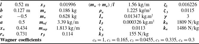
Physical characteristics and dynamic parameters of the wing section (e.g., wing and flap masses, wing and flap geometries, as well as their mass moments of inertia) for aeroelastic simulation are given in Table 1.

Table 1.

Characteristics and physical parameters of the wing section

5.1 Open loop simulation – effect of freeplay

In the open loop simulation, a wing and control surface with/without freeplay at three angles (0, 1 and 2 deg) at three airspeeds (20, 23 and 25 m/sec) and for three motions (plunge, pitch and flap deflection), including/excluding a cubic nonlinear spring in pitch are studied. Both time domain and frequency domain analysis are simulated. The simulation results are illustrated in Fig. 3 through Fig. 18.

Figure 3.

Open loop aeroelastic wing structural response for three motion modes and three airspeeds – with nonlinearity in pitch stiffness and no freeplay.

Figure 3 shows three plots representing the open-loop aeroelastic wing structural response without freeplay in three speeds and for three modes of plunge, pitch and flap deflection. The open-loop simulation result demonstrates that oscillation amplitudes are increased with increasing airspeed.

Based on the results (shown in Figs. 3 and 4) and also from Fig. 11 through Fig. 18, it is concluded that, the flutter speed of this model is roughly 23 m/s. This result has been verified by comparison with another reference [Reference Conner, Tang, Dowell and Virgin5]. Active flutter suppression, geometric control systems and real-time computational methods based on SRDE technique present by [Reference Menon, Lam, Crawford and Cheng17]. Figure 4 illustrates the time histories of open-loop aeroelastic system with freeplay 0, 1 and 2 deg at the airspeed 20 m/sec and for three modes of plunge, pitch and flap deflection. It is observed that LCO is created due to the existence of freeplay, and oscillation amplitude is increased with increasing freeplay amount.

Figure 4.

Open loop response in three modes for three freeplay cases with nonlinearity in pitch stiffness – airspeed 20 m/s.

Also, open loop aeroelastic wing structural response at the airspeed 25 m/sec and for three modes of plunge, pitch and flap deflection with control surface freeplay of 0, 1, and 2 deg are plotted in Fig. 5. It is observed that LCO phenomena are created for two cases with and without freeplay after the flutter speed.

Figure 5.

Open loop response in three modes for three freeplay cases with nonlinearity in pitch stiffness – airspeed 25 m/s.

In the Figs. 6, 7 and 8, phase planes are plotted for airspeeds 20, 23 and 25 m/s for both with and without freeplay. It can be seen from Fig. 6 (sub-flutter case), that the system states are executing LCOs for the nonlinear case ( $ \delta =2\mathrm{d}\mathrm{e}\mathrm{g}$ ). From Fig. 7 (post-flutter case), in comparison with Fig. 6, it can be seen that the amplitude of LCOs (pitch and plunge velocities) is much higher. From Fig. 8 (flutter case), it can be seen that system states are executing LCOs for both without freeplay ( $ \delta =0$ ) and with freeplay ( $ \delta =2\mathrm{d}\mathrm{e}\mathrm{g}$ ) cases.

Figure 6.

Phase plane plot for open loop response for airspeed 20 m/s.

Figure 7.

Phase plane plot for open loop response for airspeed 25 m/s.

Figure 8.

Phase plane plot for open loop response for airspeed 23 m/s.

The effect of control surface freeplay on the open loop wing structural response including a cubic nonlinear spring in pitch is illustrated in Fig. 9 through Fig. 12. As indicated, freeplay existence leads to LCO at the airspeeds under flutter speed. Also, these figures show a power spectral density (PSD) (i.e., magnitude plot) of the flap deflection which illustrate the amount of system energy at any frequency.

Figure 9.

Open loop response and power spectral density at the airspeed 20 m/s without freeplay and with a cubic nonlinear spring in pitch $(\boldsymbol{\gamma = 3})$ .

Figure 10.

Open loop response and power spectral density at the airspeed 20 m/s with freeplay and a cubic nonlinear spring in pitch $(\boldsymbol{\gamma = 3})$ .

Figure 11.

Open loop response and power spectral density at the airspeed 25 m/s without freeplay and with a cubic nonlinear spring in pitch $(\boldsymbol{\gamma = 3})$ .

Figure 12.

Open loop response and power spectral density at the airspeed 25 m/s with freeplay and a cubic nonlinear spring in pitch $(\boldsymbol{\gamma = 3})$ .

Figure 9 illustrates that, despite the non-linearity in the pitch DoF and the absence of freeplay in the flap, the flap response is slightly noisy, while the pitch response is smooth. In this special case, it seems that the flap is slightly affected by the nonlinearity of the pitch.

A comparison between Figs. 9 and 10 shows that LCO phenomena in sub-flutter responses is mainly due to flap freeplay, rather than due to cubic nonlinear spring effect. This also stands to reason, because the pitch LCO response is too small to significantly excite the cubic nonlinearity ( $ \alpha $ >> $ \gamma {\alpha }^{3}$ for alpha in radians), whereas the flap LCO response is of the same order as the freeplay gap. Cubic nonlinear spring effect in post-flutter speed on responses is illustrated in Fig. 11. Also, Fig. 12 demonstrates hybrid effect of the flap freeplay in conjunction with cubic nonlinear spring on response in post-flutter speeds. The effect of control surface freeplay on the open loop wing structural response excluding a cubic nonlinear spring in pitch is illustrated in Figs. 13 through 18.

Figure 13.

Open loop response and power spectral density at the airspeed 20 m/s without freeplay and without cubic nonlinear spring in pitch $(\boldsymbol{\gamma = 0})$ .

At sub-flutter speeds, a comparison of Fig. 13 with Fig. 16 indicates that, when control surface freeplay is included, time responses are non-convergence and LCOs are developed. Moreover, the magnitude of power spectrum density is increased. At flutter and post flutter speeds, a comparison of Fig. 14 with Fig. 17 and Fig. 15 with Fig. 18, indicates that, response modes are divergence. But, when control surface freeplay is included, the amplitudes of time response modes are increased. Furthermore, the magnitude of power spectrum density is increased.

Figure 14.

Open loop response and power spectral density at the airspeed 23 m/s without freeplay and without cubic nonlinear spring in pitch $(\boldsymbol{\gamma = 0})$ .

Figure 15.

Open loop response and power spectral density at the airspeed 25 m/s without freeplay and without cubic nonlinear spring in pitch $(\boldsymbol{\gamma = 0})$ .

Figure 16.

Open loop response and power spectral density at the airspeed 20 m/s with freeplay and without cubic nonlinear spring in pitch $(\boldsymbol{\gamma = 0})$ .

Figure 17.

Open loop response and power spectral density at the airspeed 23 m/s with freeplay and without cubic nonlinear spring in pitch $(\boldsymbol{\gamma = 0})$ .

5.2 Open loop simulation – effect of damage or reduced stiffness

In this section, the open loop response for the wing and control surface with a reduced pitch stiffness of torsional spring (due to damage), and with and without freeplay at the airspeed of 20 m/sec for three motions (plunge, pitch and flap deflection) are simulated and studied. For modeling reduced pitch stiffness, a parameter is defined as c_kα , which is reduced pitch stiffness coefficient. When c_kα is equal to one, it implies that, there is no damage. However, when c_kα is equal to 0.5, this means that stiffness of torsional spring under effects of damage is reduced to half. The effects of reduced pitch stiffness on the open loop response in two cases (i.e., with and without freeplay) for sub-flutter speed are illustrated in Fig.19 and Fig. 20, respectively.

Figure 18.

Open loop response and power spectral density at the airspeed 25 m/s with freeplay and without cubic nonlinear spring in pitch $(\boldsymbol{\gamma = 0})$ .

Figure 19.

Open loop response with reduced pitch stiffness in the case of without freeplay $(\boldsymbol{\delta = \gamma = 0})$ .

Figure 20.

Open loop response with reduced pitch stiffness in the case of with freeplay $(\boldsymbol{\delta = 2}\; {\boldsymbol{deg}},\boldsymbol{\gamma = 3})$ .

As shown in Fig. 19, due to a reduced pitch stiffness, the initial converging time responses were converted to diverging time responses. Furthermore, in Fig. 20, due to a reduced pitch stiffness, the amplitude of LCOs is considerably increased.

5.3 Closed loop simulation results – regular wing

In the closed loop simulation, the structural dynamics of the wing and control surface is studied for four cases: for a post-flutter airspeed (25 m/s) without freeplay; for a post-flutter airspeed (25 m/s) with freeplay; for a sub-flutter airspeed (20 m/s) without freeplay; and for a sub-flutter airspeed (20 m/s) with freeplay. In all four studies, time histories of three responses (plunge, pitch and flap deflection) as well as the variations of control input are plotted. The simulation results are illustrated in Figs. 21 through 24.

Figure 21.

Closed loop responses and control input for post-flutter speed without freeplay.

For the closed loop simulation, the state weighting coefficients are selected to be $ Q=\mathrm{diag}\left[\begin{array}{c@{\quad}c@{\quad}c@{\quad}c@{\quad}c@{\quad}c@{\quad}c@{\quad}c}1 {}& 10&1& 10& 1& 10& 1& 10\end{array}\right]$ and weighting factor for control input is selected to be $ $ $ R=1000$ . In SDRE, the parameter $ Q$ is the symmetric, positive semi-definite weighting matrix for states, and $ R$ is the symmetric, positive semi-definite weighting matrix for control input [Reference Hałas, Krysiak, Hałas and Stępień10].

The state dependent weighting matrices Q(x) and R(x) can be chosen to realise the desired performance objectives. In order to ensure local stability, the matrix Q(x) is required to be positive semi-definite for all x and the matrix R(x) is required to be positive definite for all x. First, weighting matrices are selected based on previous studies, and then, if performance objectives are not being met, their values are changed accordingly.

Figure 21 indicates the effectiveness of designed controller for linear aeroelastic system at the post flutter speed. Furthermore, Fig. 22 indicates the effectiveness of designed controller for nonlinear system with freeplay at the post flutter speed. All three responses are effectively controlled and damped out with a minimal control effort in about two seconds.

Figure 22.

Closed loop responses and control input for post-flutter speed with freeplay.

Comparisons between open loop and closed loop nonlinear systems for sub-flutter airspeed (20 m/s) in cases of with and without freeplay are plotted in Figs. 23 and 24, respectively. Moreover, in Figs. 25 and 26, a comparison between nonlinear open loop and closed loop responses for post-flutter airspeed (25 m/s) in cases of with and without freeplay are illustrated.

Figure 23.

A comparison between open-loop and closed-loop responses and control inputs for sub-flutter airspeed and without freeplay.

As shown in Fig. 23, in the case of without freeplay at a sub-flutter airspeed, the undamped oscillations in responses of open-loop system are damped out in the closed-loop system. The effectiveness of designed controller is more noticed, when a reduction in overshoot and a short damping time is provided.

Figure 24.

A comparison between open-loop and closed-loop responses for a sub-flutter speed and with freeplay.

As shown in Fig. 24, in the case of with freeplay at a sub-flutter airspeed, the undamped oscillations and LCOs in responses of open-loop system are damped out in the closed-loop system. The effectiveness of designed controller in an increase in the flutter speed and the suppression of the LCOs (even if it is with a higher amplitude). It is also noticed that, when the freeplay is present, the flutter speed is reduced.

Figure 25.

A comparison between open-loop and closed-loop responses for a post-flutter speed and without freeplay.

As shown in Fig. 25, in the case of without freeplay at a post-flutter airspeed, the undamped oscillations in responses of open-loop system are damped out in the closed-loop system. The effectiveness of designed controller is more noticed, when a reduction in overshoot and a short damping time is provided. The effectiveness of designed controller for LCOs suppression is very well. In this case, LCOs with more amplitudes than previous case are observed, which is due to post flutter speed.

Figure 26.

A comparison between open-loop and closed-loop responses for a post-flutter speed and with freeplay.

As shown in Fig. 26, in the case of with freeplay at a post-flutter airspeed, the undamped oscillations and LCOs in responses of open-loop system are damped out in the closed-loop system. The effectiveness of designed controller in an increase in the flutter speed and the suppression of the LCOs (even if it is with a higher amplitude). LCOs with more amplitudes than previous case are observed, which is the effect of existence of freeplay and due to post flutter speed.

5.4 Closed loop simulation results – wing with reduced stiffness

In this closed loop simulation, the structural dynamics of the wing and control surface is studied for a sub-flutter airspeed (20 m/s) in four cases; without freeplay and without a reduced pitch stiffness; without freeplay and with a reduced pitch stiffness; with freeplay and without a reduced pitch stiffness; and with freeplay and with a reduced pitch stiffness. In all four studies, time histories of three responses (plunge, pitch and flap deflection) as well as the variations of control input are plotted. As before, the reduced pitch stiffness of torsional spring is due to a damage (i.e., when c_kα = 0.5). The simulation results are illustrated and compared in Figs. 27 and 28. The effects of reduced pitch stiffness on the open loop response in two cases (i.e., with and without freeplay) are illustrated in Figs. 27 and 28, respectively.

Figure 27.

Closed loop response of the system with and without reduced pitch stiffness in the case of without freeplay.

Figure 28.

Closed loop response of the system with and without reduced pitch stiffness in the case of with freeplay.

When the pitch stiffness is reduced, the responses will experience more oscillations, as expected. However, as shown in Figs. 27 and 28, in all cases, the oscillations in responses are damped out with the application of a feedback and a controller.

Simulation results show that in the closed-loop system, the designed controller is effective in flutter suppression and a well control of motion responses. It is also shown that the control surface freeplay leads to an LCO at speeds less than linear flutter speed. Moreover, the simulation results show that the damage existence, when modeled as a reduced stiffness in torsional spring, leads to an increase in oscillation amplitudes, but does not affect the performance of designed controller. The controller is effective in suppressing the wing structural instabilities such as flutter and LCO and to keep the structure stable over a wide range of velocities.

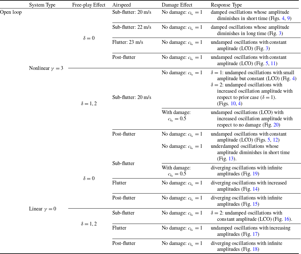
In the first and second sections of simulation – open loop – time responses are plotted based on changes on $ \delta $ , $ \gamma ,{c}_{{k}_{\alpha }}$ and airspeed. The results are summarised in Table 2.

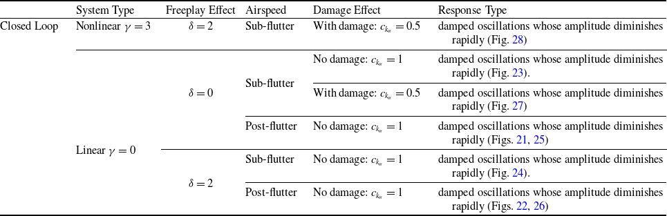
In the third and fourth sections of simulation, closed loop time responses are plotted based on changes at $ \delta $ , $ \gamma ,{c}_{{k}_{\alpha }}$ and airspeed. The results are summarised in Table 3.