1 Introduction
Electrospraying in the cone-jet mode is an atomization technique known for its ability to produce fine sprays of droplets with controllable diameters, ranging from hundreds of microns to a few nanometres (Gañán-Calvo et al.
Reference Gañán-Calvo, López-Herrera, Herrada, Ramos and Montanero2018; Rosell-Llompart, Grifoll & Loscertales Reference Rosell-Llompart, Grifoll and Loscertales2018). Typically, a liquid is fed to the tip of a capillary emitter held at high potential, and facing a grounded electrode. The liquid meniscus then becomes conical, and a jet forms at its apex from which charged droplets are emitted. The average diameter of the droplets is a function of the physical properties of the fluid and the imposed liquid flow rate
 $Q$
, and is well approximated by the characteristic scale
 $r_{c}=(\unicode[STIX]{x1D70C}\unicode[STIX]{x1D700}_{o}Q^{3}/\unicode[STIX]{x1D6FE}K)^{1/6}$
derived by Gañán-Calvo (Reference Gañán-Calvo1997);
 $\unicode[STIX]{x1D70C}$
,
 $K$
and
 $\unicode[STIX]{x1D6FE}$
stand for the density, electrical conductivity and surface tension of the liquid, and
 $\unicode[STIX]{x1D700}_{o}$
is the permittivity of the vacuum. The size distribution is narrow due to the steadiness of the jet and the capillary instability producing the droplets. The formation of the jet requires strong stresses to both balance the capillary pressure and accelerate the fluid. These forces result from the interaction of the electric field with the free and polarization charges in the fluid. Cone jets were systematically investigated for the first time by Zeleny (Reference Zeleny1914), and the conical shape of the meniscus was explained by Taylor (Reference Taylor1964). Although electrosprays can operate in a variety of regimes (Cloupeau & Prunet-Foch Reference Cloupeau and Prunet-Foch1990), the cone-jet mode (Cloupeau & Prunet-Foch Reference Cloupeau and Prunet-Foch1989) is of special interest and has been studied in great detail (Fernández de la Mora Reference Fernández de la Mora2007).
The flow rate is a key parameter in cone jets. It is adjusted to control the average diameter and charge of the droplets, the structure of the spray, the electric current, etc. The flow rate can be varied within a range, outside of which stable operation is not possible: beyond a maximum value the cone-jet mode transitions to unsteady regimes due to either the high level of charge on the surface of the jet or the inability of the jet to evacuate larger flow rates (Gañán-Calvo et al.
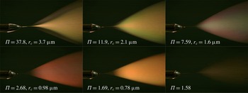
Reference Gañán-Calvo, López-Herrera, Herrada, Ramos and Montanero2018); and at sufficiently low flow rates the cone jet becomes unstable, turning on and off periodically. The goal of this article is to investigate the instability mechanism that causes the minimum flow rate. This knowledge is important because most applications benefit from operation at low flow rates: the spray is most monodisperse at this point and, as the flow increases, evolves first to a regime with two distinct populations, main and satellite droplets, followed by a regime with much broader distributions caused by the onset of lateral oscillations in the jet (Rosell-Llompart & Fernández de la Mora Reference Rosell-Llompart and Fernández de la Mora1994; Gamero-Castaño & Hruby Reference Gamero-Castaño and Hruby2002). The minimum flow rate of some fluids is so high that their cone jets can only operate in the broader regime (Gamero-Castaño Reference Gamero-Castaño2008), and understanding what triggers the instability may help solving this problem. The photographs of electrosprays in figure 1 illustrate the increasing monodispersity of the droplets at decreasing flow rate, for a solution of tributyl phosphate with an electrical conductivity of
 $100~\unicode[STIX]{x03BC}\text{S}~\text{m}^{-1}$
;
 $\unicode[STIX]{x1D6F1}$
stands for the dimensionless flow rate,
 $\unicode[STIX]{x1D6F1}=\unicode[STIX]{x1D70C}KQ/\unicode[STIX]{x1D6FE}\unicode[STIX]{x1D700}_{o}$
. For reference, note that
 $Q_{o}=\unicode[STIX]{x1D6FE}\unicode[STIX]{x1D700}_{o}/\unicode[STIX]{x1D70C}K=2.46\times 10^{-12}~\text{m}^{3}~\text{s}^{-1}$
. The average diameter of the droplets, approximately
 $1.5\cdot r_{c}$
(Gamero-Castaño Reference Gamero-Castaño2010), varies from
 $5.5~\unicode[STIX]{x03BC}\text{m}$
at the higher flow rate to
 $1.1~\unicode[STIX]{x03BC}\text{m}$
for
 $\unicode[STIX]{x1D6F1}=1.69$
. Mie scattering in this diameter range is characterized by strong scattering resonances, which expose the variation of droplet sizes through changes of colour in the spray. At the highest flow rate,
 $\unicode[STIX]{x1D6F1}=37.8$
, the spray is formed by two coaxial cones, the outer one made of the smaller satellite droplets while the inner cone carries the larger main droplets. These two populations coexist down to a flow rate
 $\unicode[STIX]{x1D6F1}=11.9$
. At lower flow rates the satellite droplets disappear. Note also the angular variation of colours in the spray for
 $\unicode[STIX]{x1D6F1}=7.59$
, which is indicative of a segregation by size of main droplets within the spray, while the droplet distribution at
 $\unicode[STIX]{x1D6F1}=2.68$
is much more monodisperse, as indicated by the homogeneous reddish hue. The two last pictures are for flow rates on both sides of the instability point,
 $\unicode[STIX]{x1D6F1}=1.69$
and
 $\unicode[STIX]{x1D6F1}=1.58$
. Monodisperse sprays are desirable for most applications, but is not the only benefit associated with low flow rate operation. For example, electrospray thrusters benefit from low flow rates not only because of improvements on thrusting efficiency associated with the monodispersity of the droplets’ charge to mass ratio
 $q/m$
, but more importantly because of increased specific impulse
 $I_{sp}$
(proportional to the exhaust velocity of the droplets), which scales with the charge to mass ratio and therefore with the flow rate as
 $I_{sp}\propto (q/m)^{1/2}\propto Q^{-1/4}$
(Gamero-Castaño & Hruby Reference Gamero-Castaño and Hruby2001).
Electrosprays of a tributyl phosphate solution with a conductivity of
 $100~\unicode[STIX]{x03BC}\text{S}~\text{m}^{-1}$
, illustrating the higher spray complexity and droplet size dispersion at increasing flow rate. The legends provide the dimensionless flow rate
 $\unicode[STIX]{x1D6F1}$
and the characteristic radius of the base of the jet
 $r_{c}$
.

An interesting feature of a cone jet is its universality, i.e. its characteristics only depend on the physical properties of the liquid and its flow rate, and are independent of geometric and electrostatic variables such as the diameter and gap between electrodes, and potential differences. This universality requires the diameter of the jet to be orders of magnitude smaller than the characteristic dimensions of the electrodes, so that the electric stress in the transition between cone and jet is largely determined by the local distribution of charge, which is effectively decoupled from the electrodes by a sufficiently large and quasi-invariant conical meniscus. In the absence of a large geometric disparity the minimum flow rate depends on the size of the emitter, the smaller the emitter the more stable the cone jet and the lower its minimum flow rate (Scheideler & Chen Reference Scheideler and Chen2014). This article focuses on the minimum flow rate condition for universal operation. In this case all non-dimensional characteristics of the cone jet are functions of three dimensionless parameters, the most common choice being the dimensionless flow rate
 $\unicode[STIX]{x1D6F1}$
, the Reynolds number
 $Re=(\unicode[STIX]{x1D70C}\unicode[STIX]{x1D700}_{o}\unicode[STIX]{x1D6FE}^{2}/\unicode[STIX]{x1D707}^{3}K)^{1/3}$
and the dielectric constant
 $\unicode[STIX]{x1D700}$
. The general dependency for the minimum flow rate is then
 $\unicode[STIX]{x1D6F1}_{min}(Re,\unicode[STIX]{x1D700})$
, and several relationships have been proposed. For example, Fernández de la Mora & Loscertales (Reference Fernández de la Mora and Loscertales1994) justify the criterion
 $$\begin{eqnarray}\displaystyle \unicode[STIX]{x1D6F1}_{min}\approx \unicode[STIX]{x1D700} & & \displaystyle\end{eqnarray}$$
on the basis of current and flow rate measurements of a number of liquids. Gañán-Calvo, Dávila & Barrero (Reference Gañán-Calvo, Dávila and Barrero1997) proposed a variation of this law,
 $$\begin{eqnarray}\displaystyle \unicode[STIX]{x1D6F1}_{min}\approx (\unicode[STIX]{x1D700}-1)^{2}, & & \displaystyle\end{eqnarray}$$
based on the hypothesis that the surface charge must be relaxed everywhere for the cone jet to be stable. Gañán-Calvo, Rebollo-Muñóz & Montanero (Reference Gañán-Calvo, Rebollo-Muñóz and Montanero2013) have proposed that a balance of opposing stresses triggers the instability. They argue that, at decreasing flow rate, the dominant force accelerating the fluid (postulated to be the pressure gradient driven by the component of the electric stress normal to the surface) is increasingly balanced by either the impeding polarization force or the impeding viscous force, depending on whether the product
 $\unicode[STIX]{x1D700}Re$
is larger or smaller than one respectively. This balance combined with scaling laws for the forces (Gañán-Calvo et al.
Reference Gañán-Calvo, Rebollo-Muñóz and Montanero2013) yield the following criterion:
 $$\begin{eqnarray}\displaystyle & \displaystyle \unicode[STIX]{x1D6F1}_{min}\approx \unicode[STIX]{x1D700},\quad \text{for }\unicode[STIX]{x1D700}Re\gg 1, & \displaystyle\end{eqnarray}$$
 $$\begin{eqnarray}\displaystyle & \displaystyle \unicode[STIX]{x1D6F1}_{min}\approx Re^{-1},\quad \text{for }\unicode[STIX]{x1D700}Re\ll 1. & \displaystyle\end{eqnarray}$$
Higuera (Reference Higuera2017) has identified the minimum flow rate condition as the characteristic flow that the electric shear stress can pull when balanced by either inertia or viscous stresses, in the presence of important relaxation effects. Higuera derives the criteria
 $$\begin{eqnarray}\displaystyle & \displaystyle \unicode[STIX]{x1D6F1}_{min}\approx \unicode[STIX]{x1D700},\quad \text{for }\unicode[STIX]{x1D700}Re\gtrsim 1, & \displaystyle\end{eqnarray}$$
 $$\begin{eqnarray}\displaystyle & \displaystyle \unicode[STIX]{x1D6F1}_{min}\approx \unicode[STIX]{x1D700}^{4}Re^{3},\quad \text{for }(\unicode[STIX]{x1D700}Re)^{3}\ll 1 & \displaystyle\end{eqnarray}$$
for polar liquids (large dielectric constant), and
 $$\begin{eqnarray}\displaystyle & \displaystyle \unicode[STIX]{x1D6F1}_{min}\approx 1,\quad \text{for }(Re/\unicode[STIX]{x1D700})^{1/3}\gtrsim 1, & \displaystyle\end{eqnarray}$$
 $$\begin{eqnarray}\displaystyle & \displaystyle \unicode[STIX]{x1D6F1}_{min}\approx \unicode[STIX]{x1D700}^{-1}Re^{3},\quad \text{for }\unicode[STIX]{x1D700}^{-1}Re^{3}\ll 1 & \displaystyle\end{eqnarray}$$
for apolar liquids (dielectric constant near one). In a recent numerical work Ponce-Torres et al. (Reference Ponce-Torres, Rebollo-Muñóz, Herrada, Gañán-Calvo and Montanero2018) determine the minimum flow rate of cone jets by performing a linear instability analysis on the solution for the base flow. This study confirms that an emitter with a small diameter helps stabilize the cone jet, and quotes a ratio of 80 between the diameters of the emitter and the jet as sufficient to eliminate the dependency of the minimum flow rate on the geometry of the electrodes. It also finds that the main instability mode develops in the transition region of the cone jet, which is consistent with the fact that other characteristics are determined by processes taking place in this local region. Ponce-Torres et al. (Reference Ponce-Torres, Rebollo-Muñóz, Herrada, Gañán-Calvo and Montanero2018) support the criterion (1.3)–(1.4).
Following this introduction, § 2 describes the experimental set-up and the methodology for measuring minimum flow rates. Two liquids with very different dielectric constants are investigated in a wide range of Reynolds numbers. The experimental
 $\unicode[STIX]{x1D6F1}_{min}(Re,\unicode[STIX]{x1D700})$
dependency highlights the importance of viscosity, and cannot be explained by criteria (1.1)–(1.5). To understand the discrepancy and find an alternative explanation the velocity, pressure, surface charge and electric fields in the cone jet are computed numerically with the continuum model described in § 3. Section 4 analyses the numerical solution, and elaborates a hypothesis for the instability mechanism based on a balance between the work done by electric stresses and the mechanical energy removed by viscous dissipation. Finally, § 5 summarizes the main findings.
2 Experimental characterization
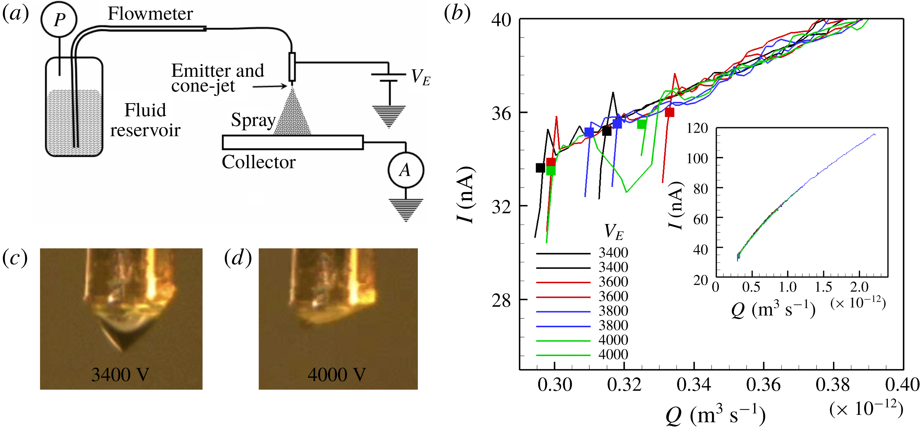
(a) Sketch of the experimental set-up. (b) Typical current versus flow rate measurements, down to the minimum stable flow rate, for a propylene carbonate solution with
 $K=0.0282~\text{S}~\text{m}^{-1}$
; each series is taken at constant emitter potential. (c,d) Geometry of the cone jet near the minimum flow rate for emitter potentials of 3400 V and 4000 V.

Figure 2 illustrates the experimental set-up and the methodology for measuring minimum flow rates. The liquid is stored in a reservoir, and fed to the emission site through two fused silica tubes connected in series by means of a zero-volume interface. The free end of the second tube is made electrically conducting with sputtered iridium and, upon applying a potential difference
 $V_{E}$
with respect to a facing collector disk, anchors the base of the cone jet, see figure 2(c,d). The outer diameter of this tube,
 $360~\unicode[STIX]{x03BC}\text{m}$
in all experiments, is also the diameter of the base of the cone jet. The flow rate is controlled by applying a known pressure to the reservoir, while the emission site is open to the atmosphere. For accurate flow rate measurement this pressure difference
 $\unicode[STIX]{x0394}P$
needs to be sufficiently high throughout the range of flow rates, which covers many orders of magnitude for the solutions investigated. To accommodate this we take advantage of the strong dependence of the flow rate on the inner diameter of the tube,
 $Q\sim D^{-4}$
, and select capillary tubes with different inner diameters depending on the solution that is electrosprayed. The fused silica tube with its free end inserted in the fluid reservoir has an inner diameter of
 $230~\unicode[STIX]{x03BC}\text{m}$
, its contribution to the overall hydraulic resistance is insignificant, and works as a flowmeter: to obtain the
 $Q(\unicode[STIX]{x0394}P)$
calibration of the line we insert air and measure the velocity at which the liquid–air interface moves at fixed
 $\unicode[STIX]{x0394}P$
. The electrospray current is measured at the collector with an electrometer, and the pressure of the reservoir with an MKS Baratron pressure transducer. Their analogue outputs are recorded with a data acquisition card, a computer and a LabView application. Figure 2(b) illustrates the characterization of the minimum flow rate for a solution of propylene carbonate with a conductivity of
 $0.0282~\text{S}~\text{m}^{-1}$
: in a typical run the emitter voltage is fixed and the reservoir pressurized to make the flow rate a few times larger than the minimum; the pressure is then slowly released through a needle valve, while recording it together with the current (see inset in figure 2
b); the recording is stopped once the electrosprays becomes unstable, as identified by the collapse of the electrospray current; these steps are repeated at several emitter potentials, and at least twice for each potential. Figure 2(b) shows current versus flow rate curves near the minimum flow rate for eight independent runs, taken at four different emitter potentials. Square symbols are indicative of the point at which the current collapses. The average of the eight minimum flow rates is
 $3.10\times 10^{-12}~\text{m}^{3}~\text{s}^{-1}$
and the relative standard deviation is 4.3 %. This narrow dispersion suggests the average value to be a deterministic output. In particular, there is no trend between the minimum flow rate of each run and the potential of the emitter. Note also that, as illustrated by figures 2(c) and 2(d), the geometry and volume of the meniscus change significantly with the emitter potential: near the instability condition the meniscus at
 $V_{E}=3400$
V remains symmetric, conical, and with an aspect ratio near one, while the meniscus at
 $V_{E}=4000$
V is highly stressed, flatter, and its apex is far from the axis of the emitter. The independency between the minimum flow rate and the geometry and size of the meniscus is to be expected from the large ratio between the radii of the emitter and the jet. The characteristic radius of the jet at the minimum flow rate is
 $r_{c}=0.080~\unicode[STIX]{x03BC}\text{m}$
, i.e. the ratio between the radii is 2250. Under these conditions the minimum flow rate is a function of the physical properties of the fluid only, and does not depend on the volume of the meniscus or the potential of the emitter.
We have measured the minimum flow rate of solutions of tributyl phosphate (TBP) and propylene carbonate (PC). The values of the density, surface tension, viscosity and dielectric constant at
 $25\,^{\circ }\text{C}$
are
 $976~\text{kg}~\text{m}^{-3}$
,
 $0.0271~\text{N}~\text{m}^{-1}$
, 0.00339 Pa s and 8.91 for tributyl phosphate, and
 $1195~\text{kg}~\text{m}^{-3}$
,
 $0.0414~\text{N}~\text{m}^{-1}$
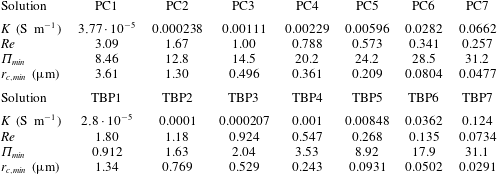
, 0.00253 Pa s and 64.9 for propylene carbonate (Riddick, Bunger & Sakano Reference Riddick, Bunger and Sakano1986). The very different dielectric constants make it possible to evaluate the effect of this parameter on the minimum flow rate. Table 1 lists the electrical conductivity of each solution (the pure liquids are doped with an ionic liquid to obtain the desired conductivity), together with the Reynolds number, the dimensionless minimum flow rate
 $\unicode[STIX]{x1D6F1}_{min}$
and the characteristic radius of the base of the jet
 $r_{c,min}$
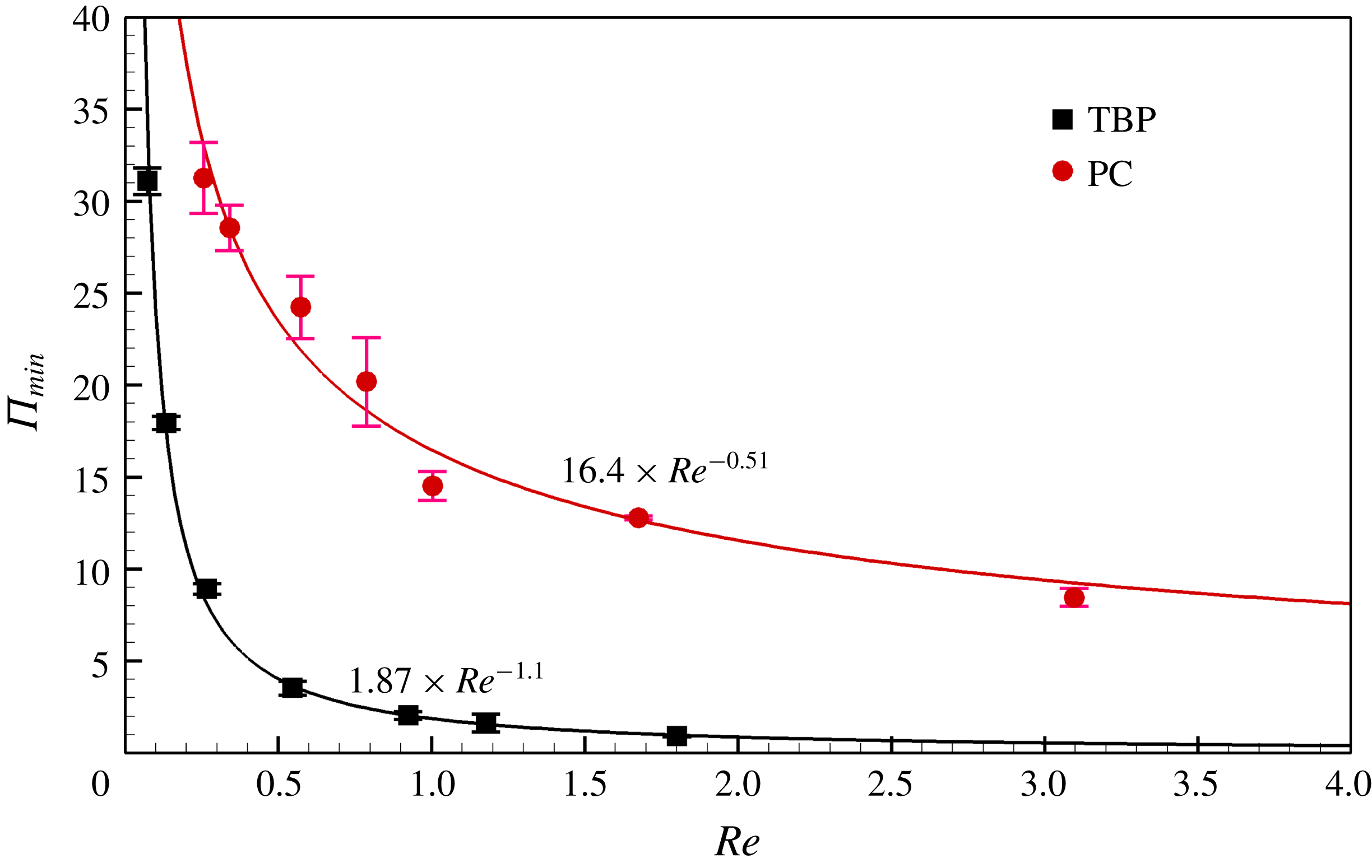
at this point. The first obvious observation is that the minimum dimensionless flow rate for both liquids increases significantly with the electrical conductivity, contrary to the predictions of every criterion except for (1.4). Figure 3 plots the minimum flow rate versus the Reynolds number. The height of the error bar is twice the standard deviation of the measurements. The minimum flow rate increases at decreasing Reynolds number for both liquids. At fixed Reynolds number propylene carbonate exhibits a significantly larger minimum flow rate than tributyl phosphate. The experimental data are incompatible with laws (1.1) and (1.2), which do not depend on the Reynolds number. The experimental data used by Fernández de la Mora & Loscertales (Reference Fernández de la Mora and Loscertales1994) and Gañán-Calvo et al. (Reference Gañán-Calvo, Dávila and Barrero1997) to justify (1.1) and (1.2) only support them as approximate criteria. For example figure 9 in Fernández de la Mora & Loscertales (Reference Fernández de la Mora and Loscertales1994) shows measurements for water at varying conductivity suggesting that
 $\unicode[STIX]{x1D6F1}_{min}$
increases at decreasing Reynolds number, similarly to what we observe in our experiments. Figure 9 in Chen, Pui & Kaufman (Reference Chen, Pui and Kaufman1995), also for water solutions at varying conductivity, suggests that
 $\unicode[STIX]{x1D6F1}_{min}$
is constant for water. However the Reynolds numbers for these solutions are between 1.28 and 3.4, i.e. they fall in the flatter section of the
 $\unicode[STIX]{x1D6F1}_{min}(Re)$
curves shown in figure 3 where
 $\unicode[STIX]{x1D6F1}_{min}$
does not change substantially. Note also that
 $\unicode[STIX]{x1D700}Re$
in figure 3 ranges between 16.0 and 0.654 for tributyl phosphate, and between 200.9 and 22.1 for propylene carbonate. Thus, the minimum flow rate criteria proposed by Gañán-Calvo et al. (Reference Gañán-Calvo, Rebollo-Muñóz and Montanero2013) and Higuera (Reference Higuera2017) seem unable to explain the experimental relationship because most investigated solutions have large
 $\unicode[STIX]{x1D700}Re$
values and would need to follow the Reynolds-independent laws (1.3) and (1.5) respectively. The disagreement is especially prominent for the propylene carbonate solutions due to their very large
 $\unicode[STIX]{x1D700}Re$
: for these very large values of
 $\unicode[STIX]{x1D700}Re$
the viscous stress should be much smaller than the polarization force in the case of Gañán-Calvo’s criterion, much smaller than inertia in Higuera’s criterion, and the Reynolds number should drop from the
 $\unicode[STIX]{x1D6F1}_{min}(Re,\unicode[STIX]{x1D700})$
relationship contrary to the experimental data in figure 3. A possible explanation of the apparent disagreement with Gañán-Calvo et al. (Reference Gañán-Calvo, Rebollo-Muñóz and Montanero2013) and Higuera (Reference Higuera2017) is that the
 $\unicode[STIX]{x1D700}Re$
values investigated may not be large enough for the inviscid limits (1.3) and (1.5) to apply. Furthermore, the Reynolds number for these solutions (and probably for most electrosprayable solutions) is never too large or too small, which limits the accuracy that can be expected from asymptotic estimations for very large or very small Reynolds numbers. Finally, we note that a second important observation from figure 3 is that the dependency on the Reynolds number requires the viscous stress to play an important role in the determination of the minimum flow rate.
Dimensionless flow rate versus Reynolds number for solutions of propylene carbonate and tributyl phosphate. The height of the error bar is twice the standard deviation of the measurement.

Electrical conductivity, Reynolds number, dimensionless minimum flow rate and characteristic radius of the base of the jet of the propylene carbonate (PC) and tributyl phosphate (TBP) solutions characterized in experiments.

3 Numerical model
We next summarize the leaky dielectric model particularized to cone jets. A detailed description of the model and the numerical algorithm can be found in Gamero-Castaño & Magnani (Reference Gamero-Castaño and Magnani2019). The variables of the model are the velocity
 $\boldsymbol{v}(\boldsymbol{x})$
and pressure
 $p(\boldsymbol{x})$
fields in the liquid, the position of the free surface
 $R(x)$
, the surface charge
 $\unicode[STIX]{x1D70E}(x)$
and the potential fields inside
 $\unicode[STIX]{x1D719}^{i}(\boldsymbol{x})$
and outside
 $\unicode[STIX]{x1D719}^{o}(\boldsymbol{x})$
the liquid. The electric field is given by
 $\boldsymbol{E}=-\unicode[STIX]{x1D735}\unicode[STIX]{x1D719}$
. The equations are expressed in dimensionless form using the scales
 $r_{c}$
,
 $v_{c}=Q/(\unicode[STIX]{x03C0}r_{c}^{2})$
,
 $p_{c}=\unicode[STIX]{x1D6FE}/r_{c}$
,
 $I_{c}=(\unicode[STIX]{x1D6FE}KQ)^{1/2}$
,
 $E_{c}=I_{c}/(\unicode[STIX]{x03C0}r_{c}^{2}K)$
,
 $\unicode[STIX]{x1D719}_{c}=r_{c}E_{c}$
and
 $\unicode[STIX]{x1D70E}_{c}=I_{c}/(2\unicode[STIX]{x03C0}r_{c}v_{c})$
. Henceforth symbols capped with a tilde will designate dimensional variables. The leaky dielectric model with constant fluid properties includes the equations of conservation of mass, Navier–Stokes and conservation of charge at the surface and the Laplace equation for the electrical potential (Melcher & Taylor Reference Melcher and Taylor1969; Saville Reference Saville1997; Higuera Reference Higuera2003):
 $$\begin{eqnarray}\displaystyle & \displaystyle \unicode[STIX]{x1D735}\boldsymbol{\cdot }\boldsymbol{v}=0,\quad \boldsymbol{v}\boldsymbol{\cdot }\unicode[STIX]{x1D735}\boldsymbol{v}=-\frac{\unicode[STIX]{x03C0}^{2}}{\unicode[STIX]{x1D6F1}^{1/2}}\unicode[STIX]{x1D735}p+\frac{\unicode[STIX]{x03C0}}{\unicode[STIX]{x1D6F1}^{1/2}Re}\unicode[STIX]{x1D6FB}^{2}\boldsymbol{v}, & \displaystyle\end{eqnarray}$$
 $$\begin{eqnarray}\displaystyle & \displaystyle \frac{\text{d}}{\text{d}x}(Rv_{s}\unicode[STIX]{x1D70E})=2RE_{n}^{i}(1+R^{\prime 2})^{1/2}, & \displaystyle\end{eqnarray}$$
 $$\begin{eqnarray}\displaystyle & \displaystyle \unicode[STIX]{x1D6FB}^{2}\unicode[STIX]{x1D719}^{i,o}=0, & \displaystyle\end{eqnarray}$$
where
 $v_{s}$
stands for the velocity at the surface,
 $E_{n}$
and
 $E_{t}$
for the components of the electric field normal and tangential to the surface and
 $x$
and
 $r$
for the axial and radial cylindrical coordinates. Additional constraints include the balance of stresses on the surface along the normal
 $\boldsymbol{n}$
and tangential
 $\boldsymbol{t}$
directions
 $$\begin{eqnarray}\displaystyle & \displaystyle p=\unicode[STIX]{x1D735}\boldsymbol{\cdot }\boldsymbol{n}-\frac{2}{\unicode[STIX]{x03C0}Re}\boldsymbol{n}\boldsymbol{\cdot }\unicode[STIX]{x1D70F}_{\unicode[STIX]{x1D707}}\boldsymbol{\cdot }\boldsymbol{n}-\frac{1}{2\unicode[STIX]{x03C0}^{2}\unicode[STIX]{x1D6F1}^{1/2}}[E_{n}^{o2}-\unicode[STIX]{x1D700}E_{n}^{i2}+(\unicode[STIX]{x1D700}-1)E_{t}^{2}], & \displaystyle\end{eqnarray}$$
 $$\begin{eqnarray}\displaystyle & \displaystyle \boldsymbol{t}\boldsymbol{\cdot }\unicode[STIX]{x1D70F}_{\unicode[STIX]{x1D707}}\boldsymbol{\cdot }\boldsymbol{n}=\frac{Re}{2}\unicode[STIX]{x1D70E}E_{t}, & \displaystyle\end{eqnarray}$$
(
 $\unicode[STIX]{x1D749}_{\unicode[STIX]{x1D707}}$
is the viscous stress tensor), the kinematic velocity condition and the jump of the normal component of the electric field at the surface
 $$\begin{eqnarray}\displaystyle \boldsymbol{v}\boldsymbol{\cdot }\boldsymbol{n}=0,\quad \unicode[STIX]{x1D70E}=\frac{2}{\unicode[STIX]{x03C0}\unicode[STIX]{x1D6F1}^{1/2}}(E_{n}^{o}-\unicode[STIX]{x1D700}E_{n}^{i}). & & \displaystyle\end{eqnarray}$$
A velocity field is prescribed at the inlet boundary (we use a homogeneous normal velocity component injecting a flow rate
 $Q$
), while the Taylor potential is imposed as the electrostatic far-field boundary condition (Taylor Reference Taylor1964; Gañán-Calvo Reference Gañán-Calvo1997; Higuera Reference Higuera2003):
 $$\begin{eqnarray}\displaystyle \unicode[STIX]{x1D719}_{T}(x,r)=-4.23\unicode[STIX]{x1D6F1}^{1/4}(x^{2}+r^{2})^{1/4}P_{1/2}\left(\frac{x}{\sqrt{x^{2}+r^{2}}}\right). & & \displaystyle\end{eqnarray}$$
Here,
 $P_{1/2}$
is the Legendre function of the first kind of degree
 $\frac{1}{2}$
. The electrostatic boundary condition is imposed on a circumference centred at the apparent vertex of the meniscus, with a dimensionless radius of
 $200\cdot \unicode[STIX]{x1D700}^{1/6}$
. The operational conditions simulated include the dielectric constants of tributyl phosphate and propylene carbonate, 8.91 and 64.9; two Reynolds numbers for each dielectric constant (0.290 and 1.12 for
 $\unicode[STIX]{x1D700}=8.91$
, and 0.396 and 0.740 for
 $\unicode[STIX]{x1D700}=64.9$
); and a wide range of flow rates for each Reynolds number, down to the minimum observed in experiments.
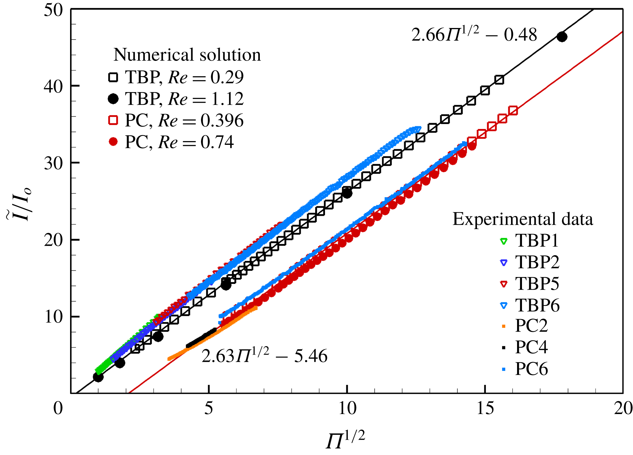
Figure 4 compares the current obtained from the model with experimental data for several solutions in table 1. The total current
 $\tilde{I}$
is the sum of the bulk conduction current
 $\tilde{I} _{B}(\tilde{x})=\int _{0}^{\tilde{R}}K\tilde{E}_{x}^{i}2\unicode[STIX]{x03C0}\tilde{r}\,\text{d}\tilde{r}$
, and the surface current
 $\tilde{I} _{S}(\tilde{x})=2\unicode[STIX]{x03C0}\tilde{R}\tilde{\unicode[STIX]{x1D70E}}\tilde{v}_{s}$
. The total current is constant along the axial coordinate due to conservation of charge. We use the scale
 $I_{o}=(\unicode[STIX]{x1D700}_{o}\unicode[STIX]{x1D6FE}^{2}/\unicode[STIX]{x1D70C})^{1/2}$
to illustrate the scaling law
 $\tilde{I} /I_{o}\propto \unicode[STIX]{x1D6F1}^{1/2}$
, which can be justified as an asymptote for large
 $\unicode[STIX]{x1D6F1}$
(Fernández de la Mora & Loscertales Reference Fernández de la Mora and Loscertales1994; Gañán-Calvo et al.
Reference Gañán-Calvo, Dávila and Barrero1997; Higuera Reference Higuera2003). The numerical results and the experimental data compare well for both liquids, supporting the validity of the model. A similar comparison by Gamero-Castaño & Magnani (Reference Gamero-Castaño and Magnani2019) yielded a good but inferior match, probably because in this case the electrosprays were operated under vacuum (Gamero-Castaño Reference Gamero-Castaño2010), with flow rates indirectly measured via time of flight. This technique is affected by uncertainties associated with the spreading of the beam and losses of mechanical energy in the cone jet (Grustan-Gutierrez & Gamero-Castaño Reference Grustan-Gutierrez and Gamero-Castaño2017), and is less reliable than the direct flow rate measurement employed in this work. The numerical solution is well fitted by the linear functions
 $\tilde{I} /I_{o}=2.66\unicode[STIX]{x1D6F1}^{1/2}-0.48$
for tributyl phosphate, and
 $\tilde{I} /I_{o}=2.63\unicode[STIX]{x1D6F1}^{1/2}-5.46$
for propylene carbonate. The Reynolds number is the weakest contributor in the
 $I(\unicode[STIX]{x1D6F1},Re,\unicode[STIX]{x1D700})$
relationship, to the point that the current of a cone jet is generally regarded as independent of the viscosity of the liquid. On the other hand the current does depend on the dielectric constant, e.g. in the
 $\tilde{I} /I_{o}\propto \unicode[STIX]{x1D6F1}^{1/2}$
scaling law this dependency appears in the form of a negative
 $y$
-intercept that becomes more significant at increasing dielectric constant.
Current versus flow rate, comparison between numerical solution and experiments. The data follow the scaling law
 $\tilde{I} /I_{o}\sim \unicode[STIX]{x1D6F1}^{1/2}$
, with
 $I_{o}=(\unicode[STIX]{x1D700}_{o}\unicode[STIX]{x1D6FE}^{2}/\unicode[STIX]{x1D70C})^{1/2}$
. The linear fits are for the numerical data.

4 Analysis of the numerical solution and discussion
We next analyse mechanisms that may cause the minimum flow rate, starting with the hypothesis that forces impeding the flow become dominant at decreasing flow rate. We will show that the algorithm is able to find numerical solutions at flow rates below the experimental minimum, especially in the case of the less polar liquid tributyl phosphate. Therefore the evidence for positive identification of the mechanism will be indirect and the theoretical conclusions somewhat speculative. The order of the analysis is reduced by using the following differential balance between jet kinetic power, pressure flow work, viscous stress flow work and the linear powers injected by the tangential electric stress on the surface and removed by viscous dissipation from the bulk (see appendix A for its derivation),
 $$\begin{eqnarray}\displaystyle \frac{\unicode[STIX]{x1D70C}Q}{2}\frac{\text{d}\langle \tilde{v}^{2}\rangle }{\text{d}\tilde{x}} & = & \displaystyle \sqrt{1+\tilde{R}^{\prime 2}}\tilde{I} _{S}\tilde{E}_{t}-Q\frac{\text{d}\langle \tilde{p}\rangle }{\text{d}\,\tilde{x}}\nonumber\\ \displaystyle & & \displaystyle +\,\frac{\text{d}}{\text{d}\,\tilde{x}}\int _{0}^{\tilde{R}}(\tilde{\unicode[STIX]{x1D70F}}_{\unicode[STIX]{x1D707}}\boldsymbol{\cdot }\boldsymbol{i}_{x})\boldsymbol{\cdot }\tilde{\boldsymbol{v}}2\unicode[STIX]{x03C0}\tilde{r}\,\text{d}\tilde{r}-\int _{0}^{\tilde{R}}(\tilde{\unicode[STIX]{x1D70F}}_{\unicode[STIX]{x1D707}}:\unicode[STIX]{x1D735}\tilde{\boldsymbol{v}})2\unicode[STIX]{x03C0}\tilde{r}\,\text{d}\tilde{r}.\end{eqnarray}$$
The averages stand for variables integrated in the cross-section of the cone jet and weighted with the axial component of the velocity, e.g.
 $\langle \tilde{p}\rangle =(1/Q)\int _{0}^{\tilde{R}}\tilde{p}\tilde{v}_{x}2\unicode[STIX]{x03C0}\tilde{r}\,\text{d}\tilde{r}$
. The dimensionless form of equation (4.1) is
 $$\begin{eqnarray}\displaystyle \underbrace{\frac{\unicode[STIX]{x1D6F1}_{Q}^{1/2}}{2\unicode[STIX]{x03C0}^{2}}\frac{\text{d}\langle v^{2}\rangle }{\text{d}x}}_{T1} & = & \displaystyle \underbrace{\sqrt{1+R^{\prime 2}}I_{s}E_{t}}_{T2}\underbrace{-\frac{\text{d}\langle p\rangle }{\text{d}x}}_{T3}\nonumber\\ \displaystyle & & \displaystyle \underbrace{+\frac{1}{\unicode[STIX]{x03C0}Re}\frac{\text{d}}{\text{d}x}\int _{0}^{R}(\unicode[STIX]{x1D70F}_{\unicode[STIX]{x1D707}}\boldsymbol{\cdot }\boldsymbol{i}_{x})\boldsymbol{\cdot }\boldsymbol{v}2\unicode[STIX]{x03C0}r\,\text{d}r}_{T4}\underbrace{-\frac{1}{\unicode[STIX]{x03C0}Re}\int _{0}^{R}(\unicode[STIX]{x1D70F}_{\unicode[STIX]{x1D707}}\boldsymbol{ : }\unicode[STIX]{x1D735}\boldsymbol{v})2\unicode[STIX]{x03C0}r\,\text{d}r}_{T5}.\end{eqnarray}$$
Strictly a power balance, (4.2) can also be interpreted as a balance of the average of forces projected on the direction of the flow. As the cone jet becomes slender (4.2) reduces to the one-dimensional momentum equation derived by Gañán-Calvo (Reference Gañán-Calvo1999) and used by Ponce-Torres et al. (Reference Ponce-Torres, Rebollo-Muñóz, Herrada, Gañán-Calvo and Montanero2018) to analyse their numerical solutions.
Numerical solution for
 $\unicode[STIX]{x1D700}=8.91$
(tributyl phosphate),
 $Re=0.29$
and two flow rates,
 $\unicode[STIX]{x1D6F1}=5.44,31.6$
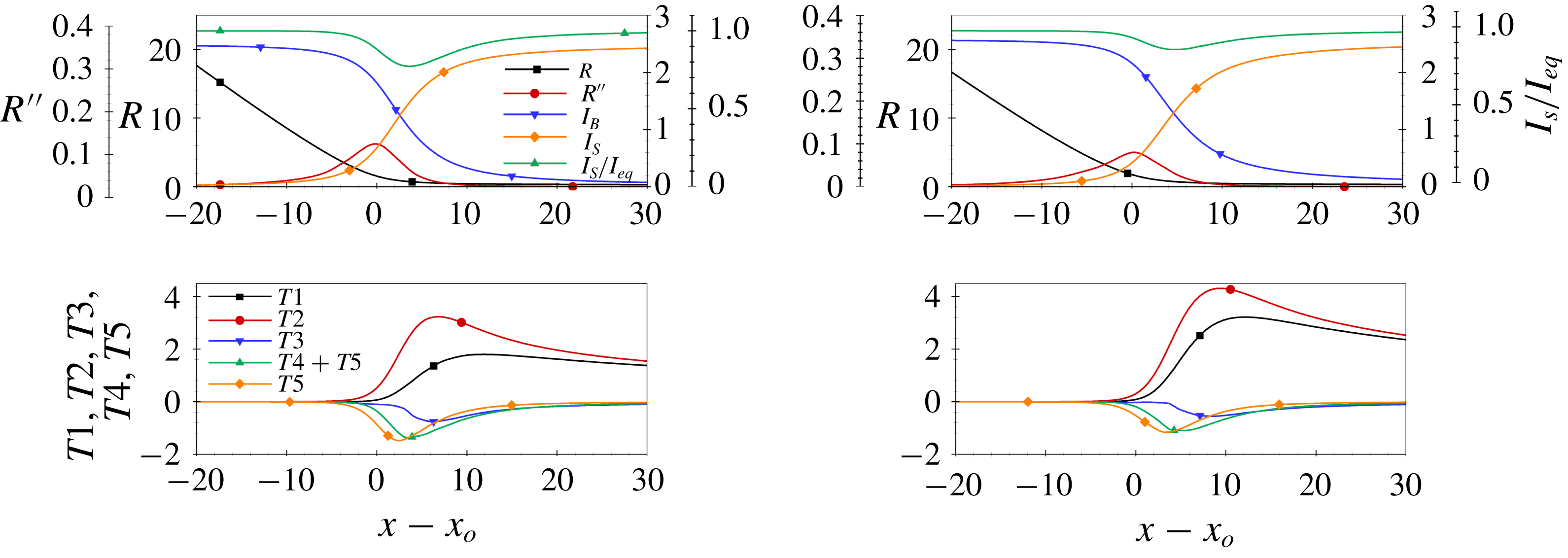
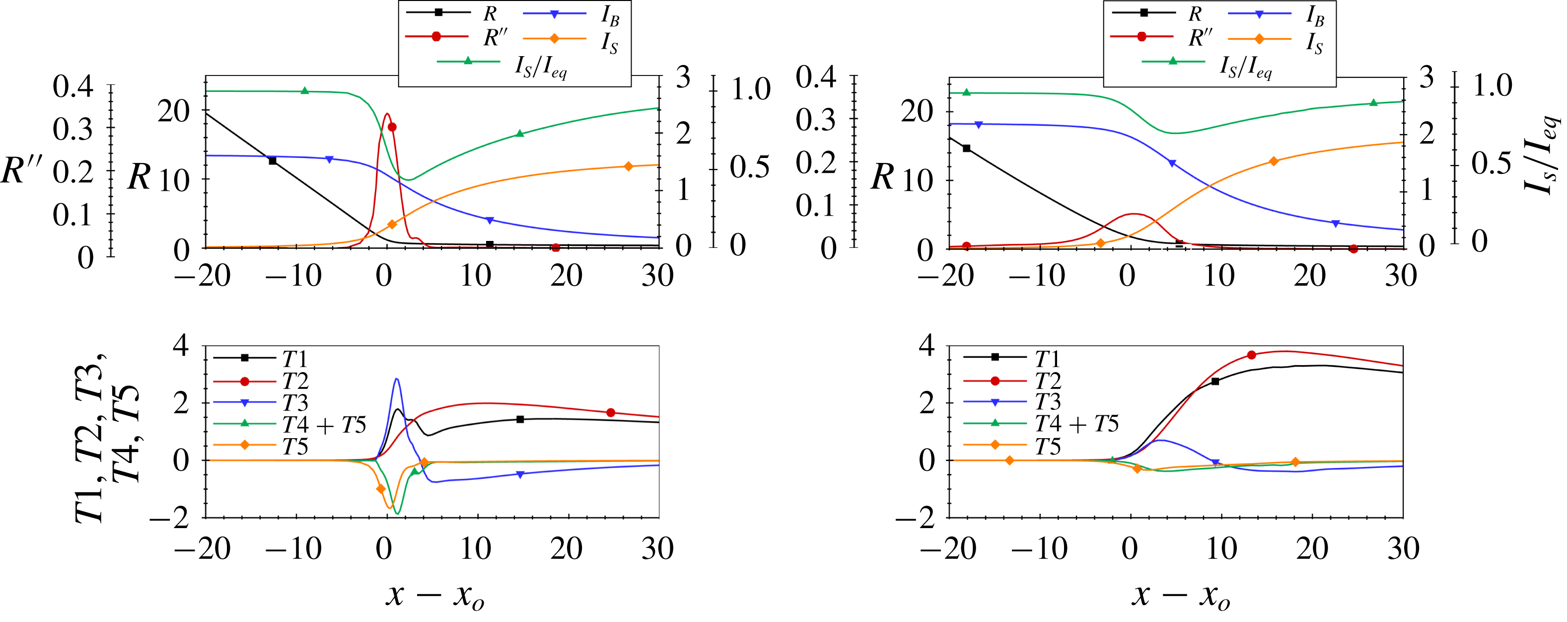
. The top charts plot the position of the surface, its second derivative, the conduction and surface currents and the ratio between the surface current and its value in equilibrium. The bottom charts plot the components of the balance (4.2).

Figure 5 illustrates the numerical solution for tributyl phosphate, a Reynolds number of 0.29 and two flow rates,
 $\unicode[STIX]{x1D6F1}=5.44$
and
 $31.6$
. The lower value is slightly smaller than the experimental minimum at this Reynolds number,
 $\unicode[STIX]{x1D6F1}_{min}=7.30$
. The top charts show the position of the surface, its second derivative
 $R^{\prime \prime }(x)$
, the bulk conduction current, the surface current and the ratio between the surface current and its value if the surface charge were in equilibrium,
 $I_{S}/I_{S,eq}=1-\unicode[STIX]{x1D700}E_{n}^{i}/E_{n}^{o}$
. In equilibrium no charge is injected on the surface from the bulk, i.e.
 $E_{n}^{i}=0$
and
 $\unicode[STIX]{x1D70E}_{eq}=2E_{n}^{o}/(\unicode[STIX]{x03C0}\unicode[STIX]{x1D6F1}^{1/2})$
. The bottom charts plot the components of the balance (4.2). The conical surface turns into a jet in an interval centred at the maximum of
 $R^{\prime \prime }$
, and using its position
 $x_{o}$
as origin of the axial coordinate helps comparing the solutions for different
 $\{\unicode[STIX]{x1D6F1},Re,\unicode[STIX]{x1D700}\}$
states. In the cone, as the liquid moves downstream the increasing surface velocity reduces the surface charge below its equilibrium value, and an electric field
 $E_{n}^{i}$
develops to inject charge on the surface and reduce the imbalance. Consequently
 $I_{B}$
decreases and
 $I_{S}$
increases in equal amounts (the total current
 $I_{B}(x)+I_{S}(x)$
remains constant). The two currents become equal at the cross-over point
 $x_{c}$
, located a few units downstream of
 $x_{o}$
. The interval within which the conduction and surface currents significantly reverse their values defines the transition region of the cone jet. In addition we define the shorter geometry transition as the interval where the cone evolves into a jet; identifiable by the significant value of
 $R^{\prime \prime }$
, it occupies the initial section of the transition region. The transition region is characterized by the absence of surface charge equilibrium (see
 $I_{S}/I_{S,eq}$
curves), to a degree that depends on the ratio between the electric relaxation time and the fluid residence time. This ratio can be cast in the form
 $\unicode[STIX]{x1D700}/\sqrt{\unicode[STIX]{x1D6F1}}$
(Gamero-Castaño & Magnani Reference Gamero-Castaño and Magnani2019), which naturally arises when rewriting equation (3.2) in terms of the surface current and the equilibrium surface current (Fernández de la Mora & Loscertales Reference Fernández de la Mora and Loscertales1994)
 $$\begin{eqnarray}\displaystyle \frac{\unicode[STIX]{x1D700}}{\unicode[STIX]{x03C0}\unicode[STIX]{x1D6F1}^{1/2}}\frac{\text{d}I_{S}}{\text{d}t}=I_{S,eq}-I_{S}, & & \displaystyle\end{eqnarray}$$
with
 $\text{d}t=\sqrt{1+R^{\prime 2}}(\text{d}x/v_{s})$
. The departure from equilibrium increases with
 $\unicode[STIX]{x1D700}/\sqrt{\unicode[STIX]{x1D6F1}}$
, so that for a liquid with low dielectric constant like tributyl phosphate the departure from full relaxation is small for most flow rates realized experimentally, and relatively significant near the minimum flow rate. The absence of charge relaxation at flow rates that are stable in experiments invalidates the hypothesis behind the criterion (1.2) for the minimum flow rate. The bottom charts in figure 5 show that the tangential electric stress and viscous stress are the dominant forces accelerating and impeding the flow respectively. The pressure increases monotonically in the direction of the flow, also impeding the motion for both flow rates. Only at very high flow rates, e.g.
 $\unicode[STIX]{x1D6F1}\gtrsim 66.5$
for
 $Re=0.290$
, the pressure develops a negative peak in the geometry transition, followed by a gradual increase to positive values. This is due to the increasing importance of the electrostatic pull, i.e. the
 $-E_{n}^{o2}/(2\unicode[STIX]{x03C0}^{2}\unicode[STIX]{x1D6F1}^{1/2})$
term in equation (3.4), and the scaling
 $E_{n}^{o}\sim \unicode[STIX]{x1D6F1}^{1/2}$
near the current cross-over point (Gañán-Calvo Reference Gañán-Calvo2004; Gamero-Castaño & Magnani Reference Gamero-Castaño and Magnani2019). The derivative of the jet kinetic power, and therefore the fluid’s acceleration, is positive throughout the transition region and increases monotonically downstream for both flow rates. Thus the average acceleration profile does not provide an indication that the flow is decelerating, much less stopping, which could make the flow unstable.
Linear electric power accelerating the flow (
 $T2$
) and total linear viscous power impeding the flow (
 $T4+T5$
) as a function of the flow rate, computed at both the current cross-over point
 $x_{c}$
and the geometry transition centre
 $x_{o}$
. Calculations are for
 $\unicode[STIX]{x1D700}=8.91$
(tributyl phosphate),
 $Re=0.29$
and
 $Re=1.12$
.

The acceleration of the flow increases monotonically downstream for all simulated flow rates of tributyl phosphate, including those below the minimum, and stays positive throughout the transition region. However the acceleration profiles do become lower at decreasing flow rate. Since a sufficiently low value of the acceleration, rather than zero, may be triggering the instability responsible for the minimum flow rate, a balance between opposing stresses could still yield the experimental dependency
 $\unicode[STIX]{x1D6F1}_{min}(Re)$
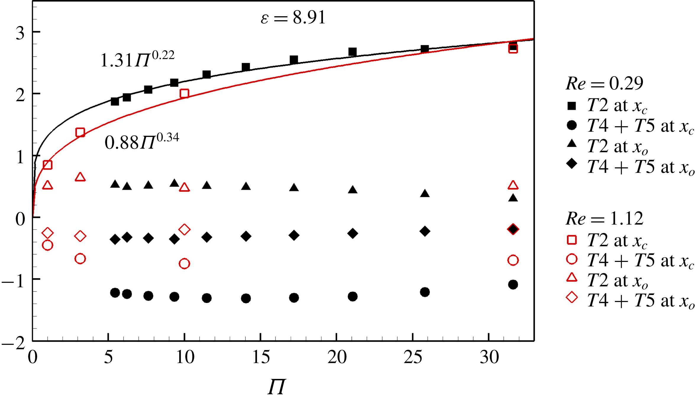
observed in figure 3. Figure 6 tests this hypothesis by plotting the linear electric power
 $T2$
accelerating the fluid and the net linear viscous power impeding it,
 $T4+T5$
, at two representative axial locations, the maximum of
 $R^{\prime \prime }$
and the current cross-over point, i.e. in the initial section of the transition region and at its centre. The data are for tributyl phosphate and two Reynolds numbers, 0.290 and 1.12. The impediment to the flow by viscous stresses is larger at
 $x_{o}$
than at
 $x_{c}$
, and remains approximately constant with flow rate. On the other hand the accelerating electric power at
 $x_{c}$
scales as
 $\unicode[STIX]{x1D6F1}_{Q}^{0.22}$
for
 $Re=0.290$
and
 $\unicode[STIX]{x1D6F1}_{Q}^{0.34}$
for
 $Re=1.12$
, while it is smaller and remains relatively constant at
 $x_{o}$
. Thus, a balance of the two dominant terms at
 $x_{o}$
suggests that it has no effect on the stability of the flow, while the balance at
 $x_{c}$
suggests the law
 $\unicode[STIX]{x1D6F1}_{min}\propto Re^{-a}$
with
 $a$
between 2.9 and 4.5. Both scenarios differ significantly from the experimental law
 $\unicode[STIX]{x1D6F1}_{min}\propto Re^{-1.1}$
.
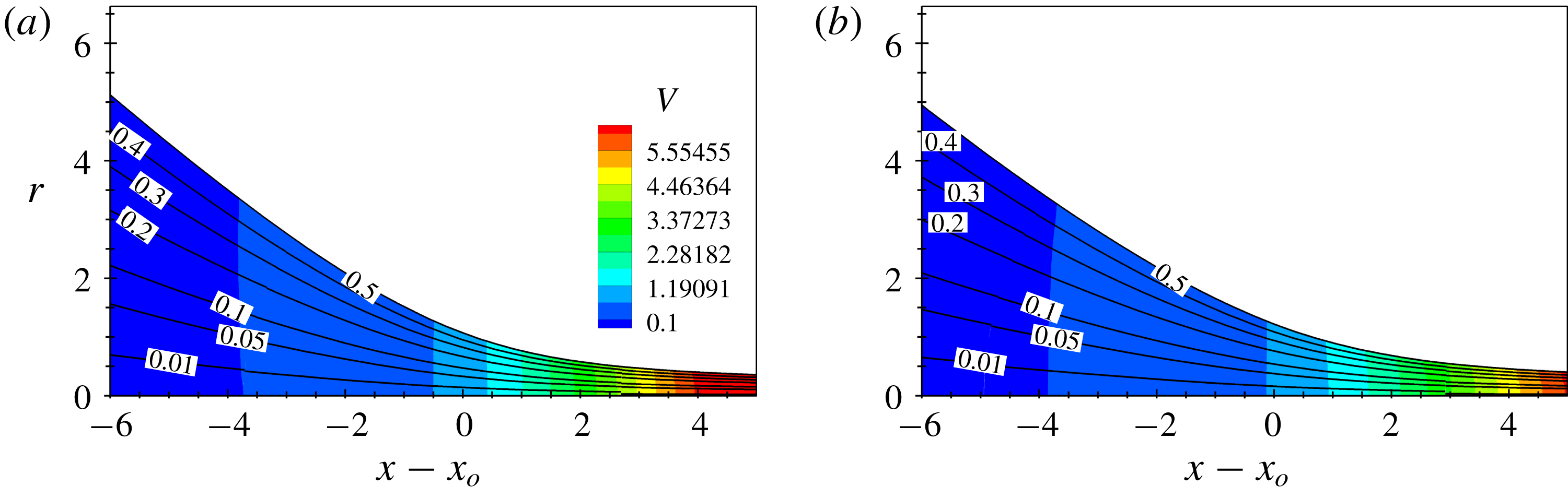
Streamlines (with values of the streamfunction) and contour map of the norm of the velocity for
 $\unicode[STIX]{x1D700}=8.91$
(tributyl phosphate),
 $Re=0.29$
and two flow rates,
 $\unicode[STIX]{x1D6F1}=5.44$
and
 $\unicode[STIX]{x1D6F1}=31.6$
.

The previous analysis suggests that the minimum flow rate is not determined by a near balance between opposing stresses. Because the integration of the variables leading to (4.2) may be suppressing two-dimensional features associated with flow deceleration and instability, figure 7 provides details of the flow field including streamlines (the streamfunction varies from 0 at the axis to
 $1/2$
at the free surface), and a contour map of the norm of the velocity. The plots extend upstream to areas where the terms in (4.2) are negligible compared to their maximum values. The streamlines are similar for both flow rates and nearly parallel to the free surface, while the norm of the velocity is almost constant at fixed
 $x$
. Thus, the flow field in the transition region is quasi-unidirectional (parallel to the free surface), changes little with the flow rate and there is no local flow deceleration nor indication that the flow may become unstable. Note also that the constant velocity norm at fixed
 $x$
everywhere in the transition region, including areas where the geometry is not slender, increases the accuracy of one-dimensional jet models like that of Gañán-Calvo (Reference Gañán-Calvo1999).
Numerical solution for
 $\unicode[STIX]{x1D700}=64.9$
(propylene carbonate),
 $Re=0.74$
and two flow rates,
 $\unicode[STIX]{x1D6F1}=30.7,200.8$
. The top charts plot the position of the surface, its second derivative, the conduction and surface currents and the ratio between the surface current and its value in equilibrium. The bottom charts plot the components of the balance (4.2).

Figure 8 shows the main features of the transition region for propylene carbonate, a Reynolds number of 0.740 and dimensionless flow rates 30.7 and 200.8. The lower flow rate is near the minimum experimental one,
 $\unicode[STIX]{x1D6F1}_{min}=19.1$
. The much larger dielectric constant of propylene carbonate has important consequences in the transition region. First, because of the larger ratio between the electric relaxation and the fluid residence times it takes a longer distance for the surface charge to equilibrate, making the transition region longer; and the surface charge falls further from equilibrium (compare the
 $I_{S}/I_{S,eq}$
profiles of both liquids), making it possible for the conical shape to extend farther towards the axis before turning into a jet. Consequently the profile of the geometry transition is much sharper, i.e. the second derivative
 $R^{\prime \prime }$
exhibits a higher peak and is narrower for large values of
 $\unicode[STIX]{x1D700}/\sqrt{\unicode[STIX]{x1D6F1}}$
(see
 $R^{\prime \prime }$
profile for
 $\unicode[STIX]{x1D6F1}=30.7$
). Second, at low flow rates the pressure gradient in (4.2) becomes the dominant accelerating term in the geometry transition, and rapidly switches to an impeding role near the current cross-over point. This is due to the
 $-(\unicode[STIX]{x1D700}-1)E_{t}^{2}/(2\unicode[STIX]{x03C0}^{2}\unicode[STIX]{x1D6F1}^{1/2})$
component of the electrostatic stress in equation (3.4) and the scaling
 $E_{t}\sim \text{constant}$
near the current cross-over point. Both combined cause a large negative pressure peak near the current cross-over at high values of
 $\unicode[STIX]{x1D700}/\sqrt{\unicode[STIX]{x1D6F1}}$
. The viscous stress remains the dominant impeding force in the geometry transition, while the electrostatic tangential stress becomes the dominant accelerating force downstream. Similarly to tributyl phosphate the acceleration of the fluid is always positive in the transition region, although at low flow rates the profile is not monotonic due to the rapid sign reversal of the pressure gradient. A balance of dominant forces at the current cross-over point cannot explain the dependence of the minimum flow rate on viscosity, because the dominant balance is between the electric tangential stress and the pressure gradient and does not include the viscous stress. Such balance could occur upstream in the geometry transition region where the viscous stress is the dominant impeding force, but in this area the accelerating pressure gradient is most intense, the acceleration of the flow exhibits a local maximum, and it is unlikely that the instability develops under the most favourable flow condition. In summary, the numerical solution suggests that the experimental dependence of the minimum flow rate on viscosity is not associated with a balance of stresses.
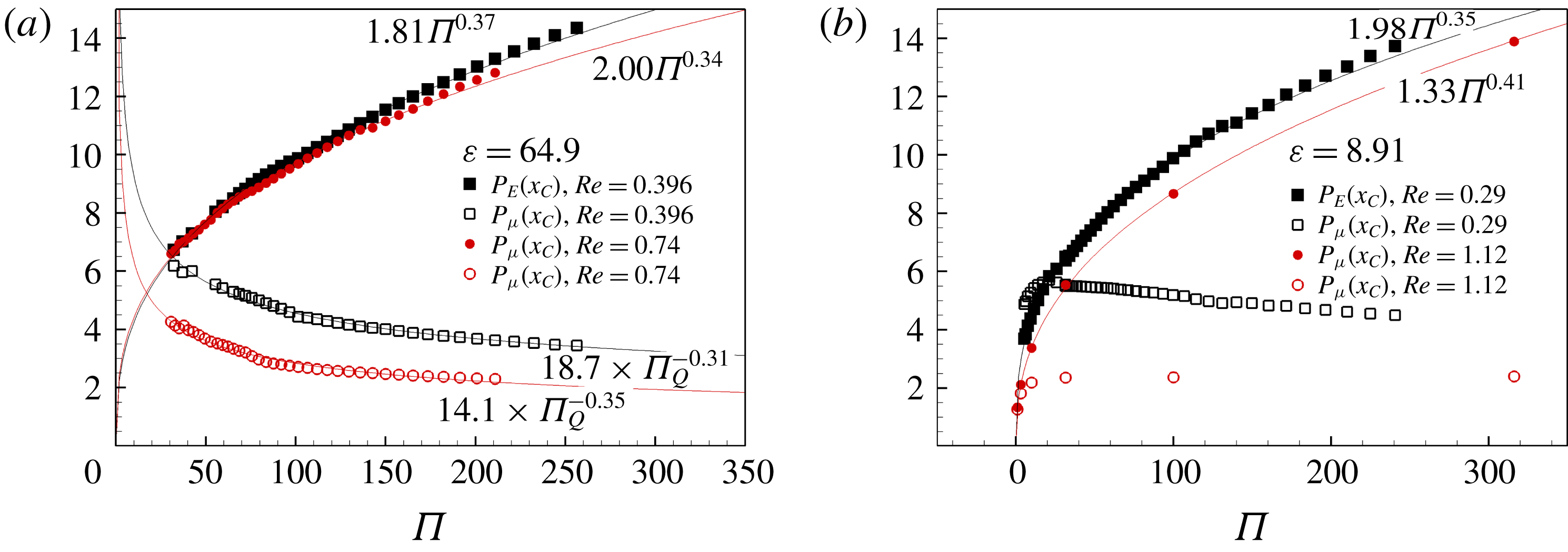
Power dissipated (
 $P_{\unicode[STIX]{x1D707}}$
) and power injected by the tangential electric stress (
 $P_{E}$
) up to the current cross-over point, as a function of the flow rate. (a) Propylene carbonate,
 $Re=0.396$
and
 $Re=0.74$
; (b) tributyl phosphate,
 $Re=0.29$
and
 $Re=1.12$
.

The dependence of the minimum flow rate on the Reynolds number requires an alternative instability mechanism with the participation of the viscous stress. The profiles in figures 5 and 8 hint at one possibility: viscous dissipation, which predominantly takes place in the geometry transition, first becomes significant upstream of the work done by the electric stress. Since the tangential electric stress is the only external force doing work on the system, it must couple with the pressure and velocity fields so that the energy that needs to be dissipated can be transferred upstream. Note also that the viscous dissipation is directly related to the geometry of the cone jet: for this quasi-one-directional flow
 $\unicode[STIX]{x2202}u/\unicode[STIX]{x2202}x$
is the larger component of the stress tensor,
 $u\approx 1/R^{2}$
, and
 $T5\approx -(1/Re)(8R^{\prime 2}/R^{4})$
. Figure 9 explores the relationship between the minimum flow rate and the injection and dissipation of mechanical energy. It shows the power dissipated up to the current cross-over point,
 $P_{\unicode[STIX]{x1D707}}(x_{c})=-\int _{-\infty }^{x_{c}}T5\,\text{d}x$
, and the power injected by the tangential electric stress,
 $P_{E}(x_{c})=\int _{-\infty }^{x_{c}}T2\,\text{d}x$
, as functions of the dimensionless flow rate. Figure 9(a) is for tributyl phosphate and
 $Re=0.290,1.12$
, and figure 9(b) is for propylene carbonate and
 $Re=0.396,0.740$
. The location of the current cross-over is significant for this analysis because it approximately bounds the region where the tangential electric stress, the viscous stress and the pressure gradient in the case of large
 $\unicode[STIX]{x1D700}/\sqrt{\unicode[STIX]{x1D6F1}}$
are comparable. Farther downstream
 $R^{\prime }$
decays rapidly decreasing the viscous dissipation density, while the bulk conduction current becomes small compared to the surface current. Both trends increase the conversion of the electric work into kinetic energy. At high flow rates the power injected up to
 $x_{c}$
, i.e. within the geometry transition, is much larger than the power dissipated. However as the flow rate decreases the difference becomes smaller and the two functions intersect at a flow rate that is comparable to the minimum one: e.g. the tributyl phosphate curves intersect at
 $\unicode[STIX]{x1D6F1}=20.1$
for
 $Re=0.290$
and
 $\unicode[STIX]{x1D6F1}=3.1$
for
 $Re=1.12$
, while the minimum flow rates are 7.3 and 1.7 respectively; and the intersection for propylene carbonate is at
 $\unicode[STIX]{x1D6F1}=31.0$
for
 $Re=0.396$
and
 $\unicode[STIX]{x1D6F1}=17.0$
for
 $Re=0.740$
, while the minimum flow rates are 26.2 and 19.1 respectively. Thus, figure 9 shows that as the flow rate decreases a larger fraction of the energy that is dissipated is being injected into the system farther downstream. The choice of
 $x_{c}$
is somewhat arbitrary, and the fitting parameters of the curves in figure 9 depend on this choice. Thus, we do not expect these fitting parameters to reproduce accurately the experimental dependency between the minimum flow rate and the Reynolds number. Furthermore a fraction of the work done by the electric stress is converted into kinetic energy. Despite this, the intersections of
 $P_{E}(x_{c})$
and
 $P_{\unicode[STIX]{x1D707}}(x_{c})$
yield
 $\unicode[STIX]{x1D6F1}_{min}=3.6Re^{-1.4}$
for tributyl phosphate and
 $\unicode[STIX]{x1D6F1}_{min}=12.7Re^{-0.96}$
for propylene carbonate, which are not very different from the experimental relationships in figure 3 and reproduce the trend of a minimum flow rate increasing with dielectric constant. The separation between the regions where power is injected and dissipated could be the mechanism making the flow unstable, as a perturbation of the flow between these two regions will alter the transfer of energy that must be dissipated, and which is fixed by the position of the surface in the geometry transition. Furthermore, the instability of the system is likely to increase with both the amount of energy that needs to be transferred and with the transfer distance, i.e. the instability is likely to increase at decreasing flow rate.
Gamero-Castaño (Reference Gamero-Castaño2019) has analysed both the ohmic and viscous dissipation taking place in cone jets to find the conditions under which self-heating is important and isothermal operation breaks down. The scaling law
 $P_{\unicode[STIX]{x1D6FA}}\cong 7.30\unicode[STIX]{x1D6F1}^{0.41}$
fits well the total ohmic dissipation in the transition region for both tributyl phosphate and propylene carbonate. The total viscous dissipation exhibits a weaker dependence on the minimum flow rate (see figure 9), and is linear in
 $Re^{-1}$
:
 $P_{\unicode[STIX]{x1D707}}\cong 2.47Re^{-1}+2.61$
for tributyl phosphate at
 $\unicode[STIX]{x1D6F1}=31.6$
, and
 $P_{\unicode[STIX]{x1D707}}\cong 1.84Re^{-1}+1.77$
for propylene carbonate at
 $\unicode[STIX]{x1D6F1}=101$
. Although the ohmic dissipation exceeds the viscous dissipation under the conditions investigated in this article, it has no effect in the balance of mechanical energy used in figure 9 because none of the mechanical work done by the electric stress is dissipated ohmically. Instead, ohmic dissipation is directly associated with the energy injected by the electric field to drive conduction current in the bulk of the liquid, none of which is transferred in the form of mechanical work (see appendix A).
We have adopted throughout the article the point of view that the minimum flow rate is triggered by a hypothetical flow instability. This is supported by the work of Ponce-Torres et al. (Reference Ponce-Torres, Rebollo-Muñóz, Herrada, Gañán-Calvo and Montanero2018) who obtain numerical solutions of the leaky dielectric model at flow rates below the minimum one, and which upon further investigation are found to be unstable. A similar inference results from our simulations of tributyl phosphate, for which we find solutions at flow rates below the minimum experimental one. On the other hand Higuera (Reference Higuera2017) argues that the minimum flow rate is an intrinsic value that the electric shear stress can pull under important charge relaxation effects, and that no solution may exist at lower flow rates. In this regard we note that convergence in our algorithm becomes increasingly difficult at decreasing flow rate near the minimum one, especially for the more polar liquid propylene carbonate. For example we have been unable to obtain solutions down to the minimum flow rate for propylene carbonate at
 $Re=0.74$
. However convergence depends on the initial shape of the profile, and it is not possible for us to say whether solutions cease to exist below a critical flow rate.
5 Conclusions
The minimum flow rate of the cone jets studied in this work is a function of the physical properties of the liquid and its flow rate, and does not depend on the potential and size of the electrodes, nor on the volume occupied by the liquid. This is due to the large disparity between the diameters of the emitter and the jet. Dimensional analysis then requires the minimum flow rate
 $\unicode[STIX]{x1D6F1}_{min}$
to be a function of at most two dimensionless parameters, the Reynolds number
 $Re$
and the dielectric constant
 $\unicode[STIX]{x1D700}$
being the typical choices. We study the function
 $\unicode[STIX]{x1D6F1}_{min}(Re,\unicode[STIX]{x1D700})$
with tributyl phosphate (
 $\unicode[STIX]{x1D700}=8.91$
) and propylene carbonate (
 $\unicode[STIX]{x1D700}=64.9$
), and vary their electrical conductivities to cover a wide range of Reynolds numbers. Contrary to existing theories (Fernández de la Mora & Loscertales Reference Fernández de la Mora and Loscertales1994; Gañán-Calvo et al.
Reference Gañán-Calvo, Dávila and Barrero1997, Reference Gañán-Calvo, Rebollo-Muñóz and Montanero2013; Higuera Reference Higuera2017), the dimensionless minimum flow rate for either liquid is not constant but increases with the electrical conductivity. In terms of the Reynolds number, the experimental data are well fitted by the power laws
 $\unicode[STIX]{x1D6F1}_{min}=1.87Re^{-1.1}$
for tributyl phosphate and
 $\unicode[STIX]{x1D6F1}_{min}=16.4Re^{-0.51}$
for propylene carbonate. Thus, the minimum flow rate increases at decreasing
 $Re$
for both liquids, and increases with the dielectric constant at fixed
 $Re$
. The dependence on the Reynolds number indicates that viscous phenomena are a key factor in the minimum flow rate condition.
The numerical solution of the leaky dielectric model (Gamero-Castaño & Magnani Reference Gamero-Castaño and Magnani2019) does not suggest that a balance of opposing forces including the viscous stress is the mechanism causing the minimum flow rate. In the case of tributyl phosphate the tangential electric stress on the surface and the viscous volumetric force are always the dominant accelerating and impeding forces respectively, but the balance yields an acceleration of the fluid that is always positive and increases monotonically along the transition region, even at flow rates below the experimental minimum. The flow field for propylene carbonate is more complicated due to its large dielectric constant which, through the polarization component of the electrostatic stress, induces a strong negative pressure peak at low flow rates. However, in the region where the viscous stress is the dominant impeding force the acceleration exhibits a local maximum, and therefore a balance based on this stress, as required by the experimental
 $\unicode[STIX]{x1D6F1}_{min}(Re,\unicode[STIX]{x1D700})$
dependence, is unlikely to make the flow unstable. An alternative instability mechanism involving the viscous stress is the significant viscous dissipation occurring in the transition from cone to jet, and which at low flow rates is not matched by the work done in the same region by the tangential electric stress. Viscous dissipation takes place predominantly in the geometry transition, immediately upstream of the current cross-over point. At high flow rates the power injected in this upstream region by the tangential electric stress, which is the only external force doing work on the cone jet, is much larger than the power dissipated; but as the flow rate decreases the difference is reduced and becomes zero at flow rates near the experimental minima. Thus, as the flow rate is reduced energy injected downstream of the current cross-over point must be increasingly transferred upstream to fulfil the dissipation required by the geometry of the cone-to-jet transition. We hypothesize that perturbations to the flow upsetting the coupling between the variables involved in the energy transfer will grow once the transferred power exceeds a threshold, i.e. at sufficiently low flow rates.
Acknowledgement
This research was supported by NASA’s Space Technology Research Early Stage Innovations program, grant NNX17AD01G.
Appendix A. Reduced-order mechanical energy equation
We next derive the reduced-order mechanical energy equation (4.2). We start with the steady state Navier–Stokes equation for an incompressible fluid in the presence of an electric field
 $$\begin{eqnarray}\displaystyle \unicode[STIX]{x1D70C}\tilde{\boldsymbol{v}}\boldsymbol{\cdot }\unicode[STIX]{x1D735}\tilde{\boldsymbol{v}}=-\unicode[STIX]{x1D735}\tilde{p}+\unicode[STIX]{x1D735}\boldsymbol{\cdot }\tilde{\unicode[STIX]{x1D70F}}_{\unicode[STIX]{x1D707}}+\unicode[STIX]{x1D735}\boldsymbol{\cdot }\tilde{\unicode[STIX]{x1D70F}}_{M}, & & \displaystyle\end{eqnarray}$$
where the electric forces acting on the fluid are modelled with the Maxwell stress tensor
 $\tilde{\unicode[STIX]{x1D749}}_{M}$
 $$\begin{eqnarray}\displaystyle \tilde{\unicode[STIX]{x1D70F}}_{M}=\unicode[STIX]{x1D700}\unicode[STIX]{x1D700}_{0}\,\tilde{\boldsymbol{E}}\tilde{\boldsymbol{E}}-\frac{1}{2}\unicode[STIX]{x1D700}\unicode[STIX]{x1D700}_{0}\left[1-\frac{\unicode[STIX]{x1D70C}}{\unicode[STIX]{x1D700}}\left(\frac{\unicode[STIX]{x2202}\unicode[STIX]{x1D700}}{\unicode[STIX]{x2202}\unicode[STIX]{x1D70C}}\right)_{T}\right]\tilde{\boldsymbol{E}}\boldsymbol{\cdot }\tilde{\boldsymbol{E}}\unicode[STIX]{x1D6FF} & & \displaystyle\end{eqnarray}$$
with associated volumetric force
 $$\begin{eqnarray}\displaystyle \unicode[STIX]{x1D735}\boldsymbol{\cdot }\tilde{\unicode[STIX]{x1D70F}}_{M}=\frac{1}{2}\unicode[STIX]{x1D700}_{0}\unicode[STIX]{x1D735}\left[\unicode[STIX]{x1D70C}\left(\frac{\unicode[STIX]{x2202}\unicode[STIX]{x1D700}}{\unicode[STIX]{x2202}\unicode[STIX]{x1D70C}}\right)_{T}\tilde{E}^{2}\right]-\frac{1}{2}\unicode[STIX]{x1D700}_{0}\tilde{E}^{2}\unicode[STIX]{x1D735}\unicode[STIX]{x1D700}+\unicode[STIX]{x1D70C}^{e}\tilde{\boldsymbol{E}}. & & \displaystyle\end{eqnarray}$$
The leaky dielectric model does not include this force in the momentum balance because to a high degree of accuracy the electrostriction force and the charge density
 $\unicode[STIX]{x1D70C}^{e}$
inside the liquid are negligible, and the dielectric constant is uniform throughout the liquid. Thus the coupling between electric forces and hydrodynamics is a surface effect, which can be enforced by requiring the free surface to be in mechanical equilibrium. The Navier–Stokes equation in the absence of electric volumetric force is multiplied (scalar product) by the velocity vector to obtain the mechanical energy equation
 $$\begin{eqnarray}\displaystyle \unicode[STIX]{x1D70C}\unicode[STIX]{x1D735}\boldsymbol{\cdot }\left(\frac{\tilde{v}^{2}}{2}\tilde{\boldsymbol{v}}\right)=-\unicode[STIX]{x1D735}\boldsymbol{\cdot }(\tilde{p}\tilde{\boldsymbol{v}})+\unicode[STIX]{x1D735}\boldsymbol{\cdot }(\tilde{\unicode[STIX]{x1D70F}}_{\unicode[STIX]{x1D707}}\boldsymbol{\cdot }\tilde{\boldsymbol{v}})-\tilde{\unicode[STIX]{x1D70F}}_{\unicode[STIX]{x1D707}}\boldsymbol{ : }\unicode[STIX]{x1D735}\tilde{\boldsymbol{v}}. & & \displaystyle\end{eqnarray}$$
This step requires the use of the continuity equation
 $\unicode[STIX]{x1D735}\boldsymbol{\cdot }\tilde{\boldsymbol{v}}=0$
and the vector identity
 $\unicode[STIX]{x1D735}(\boldsymbol{A}\boldsymbol{\cdot }\boldsymbol{B})=(\boldsymbol{A}\boldsymbol{\cdot }\unicode[STIX]{x1D735})\boldsymbol{B}+(\boldsymbol{B}\boldsymbol{\cdot }\unicode[STIX]{x1D735})\boldsymbol{A}+\boldsymbol{A}\times (\unicode[STIX]{x1D735}\times \boldsymbol{B})+\boldsymbol{B}\times (\unicode[STIX]{x1D735}\times \boldsymbol{A})$
. The last term in (A 4),
 $\tilde{\unicode[STIX]{x1D70F}}_{\unicode[STIX]{x1D707}}\boldsymbol{ : }\unicode[STIX]{x1D735}\tilde{\boldsymbol{v}}$
, is the viscous dissipation power density. Equation (A 4) is integrated in a section of the cone jet of volume
 $\unicode[STIX]{x1D6FA}$
bounded by
 $\tilde{r}-\unicode[STIX]{x1D703}$
planes at
 $\tilde{x}_{1}$
and
 $\tilde{x}_{2}$
,
 $\sum _{1}$
and
 $\sum _{2}$
, and the free surface
 $\sum _{3}$
between these planes,
 $$\begin{eqnarray}\displaystyle \int _{\unicode[STIX]{x1D6FA}}\unicode[STIX]{x1D70C}\unicode[STIX]{x1D735}\boldsymbol{\cdot }\left(\frac{\tilde{v}^{2}}{2}\tilde{\boldsymbol{v}}\right)\text{d}\tilde{V}=-\int _{\unicode[STIX]{x1D6FA}}\unicode[STIX]{x1D735}\boldsymbol{\cdot }(\tilde{p}\tilde{\boldsymbol{v}})\,\text{d}\tilde{V}+\int _{\unicode[STIX]{x1D6FA}}\unicode[STIX]{x1D735}\boldsymbol{\cdot }(\tilde{\unicode[STIX]{x1D70F}}_{\unicode[STIX]{x1D707}}\boldsymbol{\cdot }\tilde{\boldsymbol{v}})\,\text{d}\tilde{V}-\int _{\unicode[STIX]{x1D6FA}}(\tilde{\unicode[STIX]{x1D70F}}_{\unicode[STIX]{x1D707}}\boldsymbol{ : }\unicode[STIX]{x1D735}\tilde{\boldsymbol{v}})\,\text{d}\tilde{V},\qquad & & \displaystyle\end{eqnarray}$$
which, after applying the divergence theorem, becomes
 $$\begin{eqnarray}\displaystyle \int _{\unicode[STIX]{x1D6F4}_{1},\unicode[STIX]{x1D6F4}_{2}}\unicode[STIX]{x1D70C}\frac{\tilde{v}^{2}}{2}\tilde{\boldsymbol{v}}\boldsymbol{\cdot }\text{d}\tilde{\boldsymbol{A}}+\int _{\unicode[STIX]{x1D6F4}_{3}}\unicode[STIX]{x1D70C}\frac{\tilde{v}^{2}}{2}\tilde{\boldsymbol{v}}\boldsymbol{\cdot }\text{d}\tilde{\boldsymbol{A}}=-\int _{\unicode[STIX]{x1D6F4}_{1},\unicode[STIX]{x1D6F4}_{2}}\tilde{p}\tilde{\boldsymbol{v}}\boldsymbol{\cdot }\text{d}\tilde{\boldsymbol{A}}-\int _{\unicode[STIX]{x1D6F4}_{3}}\tilde{p}\tilde{\boldsymbol{v}}\boldsymbol{\cdot }\text{d}\tilde{\boldsymbol{A}} & & \displaystyle \nonumber\\ \displaystyle +\int _{\unicode[STIX]{x1D6F4}_{1},\unicode[STIX]{x1D6F4}_{2}}(\tilde{\unicode[STIX]{x1D70F}}_{\unicode[STIX]{x1D707}}\boldsymbol{\cdot }\tilde{\boldsymbol{v}})\boldsymbol{\cdot }\text{d}\tilde{\boldsymbol{A}}+\int _{\unicode[STIX]{x1D6F4}_{3}}(\tilde{\unicode[STIX]{x1D70F}}_{\unicode[STIX]{x1D707}}\boldsymbol{\cdot }\tilde{\boldsymbol{v}})\boldsymbol{\cdot }\text{d}\tilde{\boldsymbol{A}}-\int _{\unicode[STIX]{x1D6FA}}(\tilde{\unicode[STIX]{x1D70F}}_{\unicode[STIX]{x1D707}}\boldsymbol{ : }\unicode[STIX]{x1D735}\tilde{\boldsymbol{v}})\,\text{d}\tilde{V}. & & \displaystyle\end{eqnarray}$$
The second and fourth integrals are zero because the velocity at the free surface is perpendicular to the normal. Furthermore, using the balance of stresses on the free surface in the tangential direction,
 $\boldsymbol{t}\boldsymbol{\cdot }\tilde{\unicode[STIX]{x1D70F}}_{\unicode[STIX]{x1D707}}\boldsymbol{\cdot }\boldsymbol{n}=\tilde{\unicode[STIX]{x1D70E}}\tilde{E}_{t}$
, to rewrite the sixth integral in terms of the electric shear stress
 $$\begin{eqnarray}\displaystyle \int _{\unicode[STIX]{x1D6F4}_{1},\unicode[STIX]{x1D6F4}_{2}}\unicode[STIX]{x1D70C}\frac{\tilde{v}^{2}}{2}\tilde{\boldsymbol{v}}\boldsymbol{\cdot }\text{d}\tilde{\boldsymbol{A}} & = & \displaystyle -\int _{\unicode[STIX]{x1D6F4}_{1},\unicode[STIX]{x1D6F4}_{2}}\tilde{p}\tilde{\boldsymbol{v}}\boldsymbol{\cdot }\text{d}\tilde{\boldsymbol{A}}\nonumber\\ \displaystyle & & \displaystyle +\,\int _{\unicode[STIX]{x1D6F4}_{3}}\tilde{\unicode[STIX]{x1D70E}}\tilde{v}_{s}\tilde{E}_{t}\,\text{d}\tilde{A}+\int _{\unicode[STIX]{x1D6F4}_{1},\unicode[STIX]{x1D6F4}_{2}}(\tilde{\unicode[STIX]{x1D70F}}_{\unicode[STIX]{x1D707}}\boldsymbol{\cdot }\tilde{\boldsymbol{v}})\boldsymbol{\cdot }\text{d}\tilde{\boldsymbol{A}}-\int _{\unicode[STIX]{x1D6FA}}(\tilde{\unicode[STIX]{x1D70F}}_{\unicode[STIX]{x1D707}}\boldsymbol{ : }\unicode[STIX]{x1D735}\tilde{\boldsymbol{v}})\,\text{d}\tilde{V}.\qquad\end{eqnarray}$$
The surface integrals can be expressed more explicitly as
 $$\begin{eqnarray}\displaystyle & \displaystyle \int _{\unicode[STIX]{x1D6F4}_{1},\unicode[STIX]{x1D6F4}_{2}}\unicode[STIX]{x1D70C}\frac{\tilde{v}^{2}}{2}\tilde{\boldsymbol{v}}\boldsymbol{\cdot }\text{d}\tilde{\boldsymbol{A}}=\frac{\unicode[STIX]{x1D70C}Q}{2}(\langle \tilde{v}^{2}\rangle |_{\tilde{x}_{2}}-\langle \tilde{v}^{2}\rangle |_{\tilde{x}_{1}}), & \displaystyle\end{eqnarray}$$
 $$\begin{eqnarray}\displaystyle & \displaystyle \int _{\unicode[STIX]{x1D6F4}_{1},\unicode[STIX]{x1D6F4}_{2}}\tilde{p}\tilde{\boldsymbol{v}}\boldsymbol{\cdot }\text{d}\tilde{\boldsymbol{A}}=Q(\langle \tilde{p}\rangle |_{\tilde{x}_{2}}-\langle \tilde{p}\rangle |_{\tilde{x}_{1}}), & \displaystyle\end{eqnarray}$$
 $$\begin{eqnarray}\displaystyle & \displaystyle \int _{\unicode[STIX]{x1D6F4}_{3}}\tilde{\unicode[STIX]{x1D70E}}\tilde{v}_{s}\tilde{E}_{t}\,\text{d}\tilde{A}=\int _{\tilde{x}_{1}}^{\tilde{x}_{2}}\sqrt{1+\tilde{R}^{\prime 2}}\tilde{I} _{S}\tilde{E}_{t}\,\text{d}\tilde{x}, & \displaystyle\end{eqnarray}$$
 $$\begin{eqnarray}\displaystyle & \displaystyle \int _{\unicode[STIX]{x1D6F4}_{1},\unicode[STIX]{x1D6F4}_{2}}(\tilde{\unicode[STIX]{x1D70F}}_{\unicode[STIX]{x1D707}}\boldsymbol{\cdot }\tilde{\boldsymbol{v}})\boldsymbol{\cdot }\text{d}\tilde{\boldsymbol{A}}=\int _{0}^{\tilde{R}(\tilde{x}_{2})}(\tilde{\unicode[STIX]{x1D70F}}_{\unicode[STIX]{x1D707}}\boldsymbol{\cdot }\boldsymbol{i}_{x})\boldsymbol{\cdot }\tilde{\boldsymbol{v}}2\unicode[STIX]{x03C0}\tilde{r}\,\text{d}\tilde{r}-\int _{0}^{\tilde{R}(\tilde{x}_{1})}(\tilde{\unicode[STIX]{x1D70F}}_{\unicode[STIX]{x1D707}}\boldsymbol{\cdot }\boldsymbol{i}_{x})\boldsymbol{\cdot }\tilde{\boldsymbol{v}}2\unicode[STIX]{x03C0}\tilde{r}\,\text{d}\tilde{r}. & \displaystyle\end{eqnarray}$$
The averages stand for variables integrated in the cross-section and weighted with the axial component of the velocity, e.g.
 $\langle \tilde{p}\rangle =(1/Q)\int _{0}^{\tilde{R}}\tilde{p}\tilde{v}_{x}2\unicode[STIX]{x03C0}\tilde{r}\,\text{d}\tilde{r}$
. The symmetry of the viscous stress tensor allows us to change the order of the inner products in
 $(\tilde{\unicode[STIX]{x1D749}}_{\unicode[STIX]{x1D707}}\boldsymbol{\cdot }\tilde{\boldsymbol{v}})\boldsymbol{\cdot }\boldsymbol{i}_{x}$
, (A 11). Using now a differential cross-section of the cone jet as the control volume in (A 7),
 $\tilde{x}_{2}=\tilde{x}_{1}+\text{d}\tilde{x}$
, and taking a derivative in
 $\tilde{x}$
, yields the following differential balance:
 $$\begin{eqnarray}\displaystyle \frac{\unicode[STIX]{x1D70C}Q}{2}\frac{\text{d}\langle \tilde{v}^{2}\rangle }{\text{d}\,\tilde{x}} & = & \displaystyle \sqrt{1+\tilde{R}^{\prime 2}}\tilde{I} _{S}\tilde{E}_{t}-Q\frac{\text{d}\langle \tilde{p}\rangle }{\text{d}\,\tilde{x}}\nonumber\\ \displaystyle & & \displaystyle +\,\frac{\text{d}}{\text{d}\,\tilde{x}}\int _{0}^{\tilde{R}}(\tilde{\unicode[STIX]{x1D70F}}_{\unicode[STIX]{x1D707}}\boldsymbol{\cdot }\boldsymbol{i}_{x})\boldsymbol{\cdot }\tilde{\boldsymbol{v}}2\unicode[STIX]{x03C0}\tilde{r}\,\text{d}\tilde{r}-\int _{0}^{\tilde{R}}(\tilde{\unicode[STIX]{x1D70F}}_{\unicode[STIX]{x1D707}}\boldsymbol{ : }\unicode[STIX]{x1D735}\tilde{\boldsymbol{v}})2\unicode[STIX]{x03C0}\tilde{r}\,\text{d}\tilde{r}\end{eqnarray}$$
between the jet kinetic power, the power per unit length injected by the electric shear stress on the surface, the pressure flow work, the viscous stress flow work and the power per unit length removed by viscous dissipation, respectively. The dimensionless form of equation (A 12) is
 $$\begin{eqnarray}\displaystyle \frac{\unicode[STIX]{x1D6F1}_{Q}^{1/2}}{2\unicode[STIX]{x03C0}^{2}}\frac{\text{d}\langle v^{2}\rangle }{\text{d}x} & = & \displaystyle \sqrt{1+R^{\prime 2}}I_{s}E_{t}-\frac{\text{d}\langle p\rangle }{\text{d}x}\nonumber\\ \displaystyle & & \displaystyle +\,\frac{1}{\unicode[STIX]{x03C0}Re}\frac{\text{d}}{\text{d}x}\int _{0}^{R}(\unicode[STIX]{x1D70F}_{\unicode[STIX]{x1D707}}\boldsymbol{\cdot }\boldsymbol{i}_{x})\boldsymbol{\cdot }\boldsymbol{v}2\unicode[STIX]{x03C0}r\,\text{d}r-\frac{1}{\unicode[STIX]{x03C0}Re}\int _{0}^{R}(\unicode[STIX]{x1D70F}_{\unicode[STIX]{x1D707}}\boldsymbol{ : }\unicode[STIX]{x1D735}\boldsymbol{v})2\unicode[STIX]{x03C0}r\,\text{d}r.\qquad\end{eqnarray}$$
This reduced-order mechanical energy equation shows that the work done by the electric shear stress (this work is always positive) both increases the kinetic energy of the fluid and supplies the energy dissipated by the viscous stress. The pressure flow work and the viscous stress flow work can be locally significant at the base of the jet, and their signs typically reverse along this region. They can be thought of mechanisms for transferring and converting the work done by the electric field into both kinetic energy and viscous dissipation. We write transferring because the axial location where the electric field does most of the mechanical work does not necessarily coincide with the region where viscous dissipation is most intense, in fact these regions increasingly separate at decreasing flow rate. It is worth noting that stresses normal to the surface do not enter in this balance because they do not do work on the fluid. Ohmic dissipation is not part of this mechanical energy balance either, although it can be introduced in a similar balance together with additional terms (Gamero-Castaño Reference Gamero-Castaño2010). The ohmic dissipation power density
 $K\tilde{E}^{2}$
can be integrated in any volume of fluid to show that it is equal to the electrical power driving the electric current through its boundary
 $$\begin{eqnarray}\displaystyle \int _{\unicode[STIX]{x1D6FA}}K\tilde{E}^{2}\,\text{d}\tilde{V}=-\int _{\unicode[STIX]{x1D6FA}}\unicode[STIX]{x1D735}\boldsymbol{\cdot }(\tilde{\unicode[STIX]{x1D719}}K\tilde{\boldsymbol{E}})\,\text{d}\tilde{V}=-\int _{\unicode[STIX]{x1D6F4}}\tilde{\unicode[STIX]{x1D719}}\tilde{\boldsymbol{J}}\boldsymbol{\cdot }\text{d}\tilde{\boldsymbol{A}}, & & \displaystyle\end{eqnarray}$$
where
 $\tilde{\boldsymbol{J}}$
is the current density,
 $\tilde{\boldsymbol{J}}=K\tilde{\boldsymbol{E}}$
. We make use here of a constant electrical conductivity and zero charge density inside the fluid. Equation (A 14) shows that the power injected by the electric field in any control volume inside the liquid (third integral) is equal to the ohmic dissipation in the control volume (first integral). This is to be expected from the negligible volumetric force inside the liquid associated with the Maxwell stress: the electric field in the bulk of the liquid cannot do mechanical work and all the energy it transfers must be converted into heat (ohmic dissipation).