Physical setting

Recent research by participants in the Siple Coast Project has produced exciting new glaciological data from Ice Stream B and its surroundings (e.g. Reference BentleyBentley, 1987; Reference BentleyBentley and others, 1987; Reference Bindschadler, Stephenson, MacAyeal and ShabtaieBindschadler and others, 1987; Reference MacAyeal, Bindschadler, Shabtaie, Stephenson and BentleyMacAyeal and others, 1987; Reference Shabtaie and BentleyShabtaie and Bentley, 1987; Reference Shabtaie, Whillans and BentleyShabtaie and others, 1987; Reference Whillans, Bolzan and ShabtaieWhillans and others, 1987; Reference Alley and BentleyAlley and Bentley, 1988; see part I, Fig. 1). The ice stream carries the accumulation of a large section of West Antarctica across the Siple Coast and into the Ross Ice Shelf. It is recognizable for about 400 km along flow, but the last 100 km are an “ice plain” with very low, almost ice-shelf-like surface slopes. In the upper 150 km the ice stream has two main branches separated by a slower-moving ridge, but ice from the branches is distinct down-stream of their junction. The entire drainage system of Ice Stream B shows a significantly negative mass balance, probably attributable in large part to thinning associated with headward growth of the ice stream into its catchment area. Ice velocities are high (≈500 m a⁻¹) despite low driving stresses (≈20 kPa); ice thicknesses are near 1000 m, and the bed is roughly horizontal along flow. Accumulation rates on the ice stream and in much of its catchment area are low (≈100 mm ice a⁻¹). Temperatures are low (≈–26°C), surface melt is rare, and no run-off occurs.

Fig. 1.

Smoothed, two-dimensional version of Ice Stream B used in model calculations. Modified from Reference Alley, Blankenship, Rooney and BentleyAlley and others (1987c).

Much information also has been obtained about the geological setting of Ice Stream B. The ice stream generally follows the axis of a subglacial trough tens to hundreds of meters deep, although exact correspondence is not maintained between the margins of the trough and the ice stream (Reference Shabtaie, Whillans and BentleyShabtaie and others, 1987). The trough probably is structurally controlled but modified by glacial erosion (Rooney and others, 1987Reference Rooney, Blankenship, Bentley and McKenziea,b). Beneath the meters thick subglacial till, the ice stream is underlain by hundreds of meters of sedimentary rocks with low seismic velocities; based on available geological data and analogy to geophysical properties of sediments beneath the Ross Sea, these probably are poorly indurated, Neogene glaciomarine sediments (Reference Rooney, Blankenship, Alley and BentleyRooney and others, 1989).

. One of the more exciting results of the Siple Coast Project has been the discovery of a subglacial substrate that on the basis of geophysical evidence is probably a meters thick, unconsolidated layer beneath the ice stream near the Upstream B camp (UpB; see part I, Fig. 1), characterized by high porosity and high pore-water pressure (Blankenship and others, Reference Blankenship, Bentley, Rooney and Alley1986,1987; Reference Rooney, Blankenship, Alley and BentleyRooney and others, 1987b). The layer is known to occur over a 10 km by 10 km area near UpB (Reference Rooney, Blankenship, Alley and BentleyRooney and others, 1988); preliminary interpretation of seismic data collected near the Downstream B camp (DnB, part I, fig. I) about 200 km down-stream, suggests that the same layer occurs there with similar thickness (Reference Blankenship, Rooney, Alley and BentleyBlankenship and others, 1989). We have argued that this layer probably is deforming pervasively beneath the ice stream and causing most of the ice velocity (Alley and others, Reference Alley, Blankenship, Bentley and Rooney1986,1987a,b,c).

This layer is similar, in thickness and stratigraphie relation to other units, to the widespread till overlying the Ross Sea unconformity beneath the Ross Sea (Reference BarrettBarrett, 1975; Reference Anderson, Kurtz, Domack and BaishawAnderson and others, 1980; Reference Karl, Reimitz and EdwardsKarl and others, 1987). This similarity, plus our hypotheses about till deformation and its effect on ice-sheet history, have led us to suggest that the layer beneath Ice Stream B and the Ross Sea till had the same origin, that the Ross Sea till records Wisconsinan ice-stream flow in an expanded ice sheet, and that the layer beneath Ice Stream B is a till like that in the Ross Sea (Reference Alley, Blankenship, Rooney and BentleyAlley and others, 1989).

The amount of detailed data available regarding Ice Stream B exceeds our present capability to understand or model it (although Reference MacAyealMacAyeal (in press),Whillans and Van der Veen (1989), and others are making excellent progress). To isolate the effects of basal processes, it is convenient to simplify the system drastically.

We thus consider the idealized, two-dimensional, steady ice stream shown in Figure 1, from Reference Alley, Blankenship, Rooney and BentleyAlley and others (1987c). The head of this idealized ice stream is at x = 0, and the coupling line between the main part of the ice stream and the ice plain is at x = 300 km; we defer the problem of flow beyond the coupling line to a later study. Surface slope is constant at α_s = 0.002, bed slope is constant at = 0, and accumulation rate is constant at b = 0.1 ma⁻¹ of ice. The UpB camp is at x = 100km, where the ice thickness is h = 1050 m, the ice velocity is u _iB = 448 m a⁻¹ and the deforming till thickness is Z₁ = 6 m. Velocity from internal ice deformation is assumed to be negligible, and the driving stress is assumed to be balanced by the basal shear stress. From this, we can calculate the basal velocity and basal shear stress everywhere along the model ice stream (Reference Alley, Blankenship, Rooney and BentleyAlley and others, 1987c; also Fig. 2). The preliminary observations of Reference Blankenship, Rooney, Alley and BentleyBlankenship and others (1989) and the model results of Reference Alley, Blankenship, Rooney and BentleyAlley and others (1987c) suggest that till thickness does not vary rapidly along flow, so we assume Z₁ = 6 m to apply to the entire length. The effect of probable errors in these assumptions is discussed in the sub-section on sensitivity, below, and in Reference Alley, Blankenship, Rooney and BentleyAlley and others (1987c).

Fig. 2.

Calculated values of important variables along model ice stream in Figure 2. The head of the ice stream is at x = 0 km and UpB is at x = 100 km. T_B = basal shear stress, d = water-film thickness, U₁ = ice velocity, u_s/u_sB = ratio of sliding velocity (u_s) to sliding velocity at UpB (u_sB), q = water flux at ice—till interface, and N = effective pressure.

As noted above, it is likely that the layer beneath Ice Stream B is a till similar to that observed in the Ross Sea (Reference Alley, Blankenship, Rooney and BentleyAlley and others, 1989). A reasonable approximation to the measured grain-size distribution of that material (Reference BarrettBarrett, 1975; Reference Anderson, Kurtz, Domack and BaishawAnderson and others, 1980) is that clasts fall into seven size classes with radii Rj = 10⁻⁶, 10⁻⁵, …, 10°m with one-tenth of the volume in each of the seven size classes and with the remaining 30% of the volume assumed to be in pores (cf. Reference Boulton and HindmarshBoulton and Hindmarsh, 1987). This probably overestimates the volume fraction in the two coarsest classes, but is convenient and is not a bad approximation. Seismic measurements on Ice Stream B show that roughness elements at the 10 m vertical scale are absent or scarce, especially parallel to flow (Reference Rooney, Blankenship, Alley and BentleyRooney and others, 1987b). We initially assume that this subglacial till rests directly on rigid bedrock, although later we relax this assumption somewhat.

Water system

Calculations for Ice Stream B show that it generates much more water than could be conducted through likely subglacial aquifers (Reference Linge and BrownLingle and Brown, 1987) or advected in a deforming bed (Reference Alley, Blankenship, Bentley and RooneyAlley and others, 1987b), so drainage must occur at the ice-bed interface. As discussed in part I, such drainage over an unconsolidated bed beneath a cold glacier is likely to occur in an inefficient, distributed system with an effective pressure of only 0(10⁴Pa). Although this water system is likely to evolve rapidly, with growth and collapse of local thickenings, we hypothesized in part I that it will resemble a perturbed film more than channelized drainage.

We thus choose to model the water flow as occurring through a Weertman film (Reference WeertmanWeertman, 1972; Reference Weertman and BirchfieldWeertman and Birchfield, 1982). The thickness, d, of such a Weertman film is (see part I, equation (25))

where μ = 1.8 χ 10⁻³Pa s is the viscosity of water, q is the water flux in m³/s per meter width, and is the pressure-gradient driving flow. For the assumed configuration of Ice Stream B (see part I, equation (26))

where P_i ≈ 910 kg m⁻³ is the ice density, g = 9.8 ms⁻² is the gravitational acceleration, and a_s = 0.002 is the ice-air surface slope.

The water flux at the ice-bed interface, q, is the sum of water entering the head of the ice stream at the ice—bed interface, q_i and the water generated along the ice stream that is not lost to conduction or advection through subglacial aquifers. Model results show that q_i ≪ q except possibly in the first tens of kilometers (Reference Budd and JenssenBudd and Jenssen, 1987), so we take ˃ ¡ = 0. Also, water flux from the ice-bed interface into subglacial aquifers along the ice stream is likely to be small compared to q (Reference Alley, Blankenship, Bentley and RooneyAlley and others, 1987b; Reference Linge and BrownLingle and Brown, 1987) so we take it to be zero. Heat conduction through the ice stream is about equal to the geothermal flux (Reference Alley and BentleyAlley and Bentley, 1988) so q is generated by the heat of sliding.

Basal melting from the heat of sliding occurs at a rate v _m given by

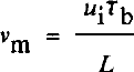
where u _i is the basal ice velocity, is the basal shear stress, and L = 3.1 χ 10⁸Jm⁻³ is the heat fusion of ice. Then

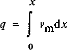
for q_i = 0. Values of q calculated from Equation (4) are shown in Figure 2. The water-film thickness, d, then can be calculated from Equations (1) and (2), and also appears in Figure 2.

In part II (equations (2) and (3)) we discussed the relation between water-film thickness and the fraction of the bed, /, occupied by the water film. Equation (3) in part II was derived for the bed roughness that we argue above is most likely to occur beneath Ice Stream B. We thus expect Ice Stream B to be described by

where d is in meters. In part I we argued that a bed containing abundant roughness elements in a wide range of sizes, such as that assumed here, will have a relation between /, T^, and effective pressure N (the difference between the average normal stress of ice on the bed and the water pressure) given by (part I, equation (22))

where β is a geometric constant related to the bed roughness. If we take N = 50 kPa at UpB from Reference Blankenship, Bentley, Rooney and AlleyBlankenship and others (1987), then Equations (5), (6), and the calculated values of and d at UpB allow us to estimate ß. The values of T_b and d along the ice stream (Fig. 2) then allow us to calculate N along the ice stream for constant β. The result is that β ≈ 2, leading to the values of N shown in Figure 2.

Sliding and bed deformation

The calculated water-film thicknesses (Fig. 2) are typically several millimeters, similar to the controlling obstacle size for sliding under these conditions (Reference WeertmanWeertman, 1964; see part I, equation (27), and part II, equation (4)). This allows the sliding velocity, u_s, to be approximated as

where K_s ≈ 2 χ 10⁻⁶ (m a⁻¹) Pa⁻² m⁻¹ based on Reference WeertmanWeertman (1964) sliding theory as discussed for equation (4) in part II. Equation (7) yields a sliding velocity of about 3 m a⁻¹ at UpB. Assuming that K_s is constant along the ice stream (that is, that the roughness of the ice-bed interface does not vary along flow), the variation in sliding velocity along flow comes from variation in and d, and is shown in Figure 2. Weertman sliding theory allows some latitude in calculating K_s (e.g. Weertman, Reference Weertman1964,1969) because of uncertainties regarding exact conditions at the bed; however, it is difficult to construct a scenario in which u_s accounts for a significant fraction of the total ice velocity over the assumed bed.

We thus model the ice stream assuming that most of the ice velocity arises from deformation in the bed. Although ploughing and discrete shearing may account for some velocity, at Breidamerkurjökull most of the velocity arises from pervasive deformation (Reference Boulton and HindmarshBoulton and Hindmarsh, 1987). We will start by assuming that all of the deforma-tional velocity arises from pervasive shear, and that this shear obeys the flow law (part II, equation (24))

where z and u are depth and horizontal velocity in till, respectively, K_b, a, and b are constants, and τ* is the shear strength of till.

We will follow the preferred path of Reference Boulton and HindmarshBoulton and Hindmarsh (1987) in modeling Equation (8) with τ* = 0 and N independent of z initially. This approach reveals the interesting features of the system more clearly and, as discussed in the sub-section on sensitivity, it can be generalized easily. Reference Boulton and HindmarshBoulton and Hindmarsh (1987) measured N near the ice-till interface, calculated its variation with depth in the till, and obtained an average value of N to use in comparisons between sites; allowing N to vary with depth produces model results that can be related directly to this fixed N case, as shown below. The total velocity, U₀, arising from the deformation in a till layer Z₁ thick then is

where the average is taken over the deforming till thickness. Because the till thickness (6 m) is much less than the ice thickness (≈1000 m), T_b is nearly independent of z in the till, and we make the thin-till approximation that is independent of z. Then, if N is independent of z, du/dz is a constant and the average in Equation (9) is unnecessary.

Model

Equations (1)–(9) plus the assumptions embedded in the discussion of these equations provide a complete description of the basal velocity of a cold, two-dimensional, wet-based glacier flowing on a deforming bed, provided that the ice and till geometries (till thickness and basal shear stress) are known. Equations (7)–(9) yield the basal velocity, u _i, when combined with

Equations (1)–(6) show how the water system determines the effective pressure, N, and the water-film thickness, d, and thus the deformational velocity, u₀, and the sliding velocity, u _s.

The system specified here is quite simple, but we believe that it incorporates most of the real behavior of an ice stream on deforming till. The grain-size distribution of a till controls the roughness of its upper surface, and thus the sliding softness, K_s, as well as the details of internal shear, and thus the deformational softness, K_b. The interaction of the water supply with the basal shear stress, the pressure-gradient driving water flow, and the roughness of the upper surface of the bed produces a unique average water-film thickness and effective pressure at the ice-bed interface. The sliding softness, water-film thickness, and basal shear stress then yield the sliding velocity, and the deformational softness, effective pressure, till thickness, and basal shear stress yield the deformational velocity; the sum of these two is the basal ice velocity.

Our approach is to use Equations (1)–(6) to estimate N and d, and to obtain to and T_b from the idealized version of the ice stream described above and shown in Figures 1 and 2. If the constants a, b, ß, K_s, and K_b were known independently, then they would provide a second estimate of Uj from Equations (7)-(10). Unfortunately, although we can limit the values of these constants, none is known exactly. We will limit these constants as closely as possible, and then determine which combination(s) within the limits reproduce the idealized ice stream best.

The tills beneath the Ross Sea above the Ross Sea unconformity are not strongly variable spatially (Reference Anderson, Kurtz, Domack and BaishawAnderson and others, 1980), and we argued above that the tills beneath Ice Stream B are likely to be similar. We thus assume that the grain-size distribution is independent of position (horizontal and vertical) in the deforming till beneath Ice Stream B, and that K_b, K_s, and β are independent of position as well.

The constant β can be estimated from Equation (6) using the seismically estimated effective pressure of N = 50 ± 40 kPa at UpB (Reference Blankenship, Bentley, Rooney and AlleyBlankenship and others, 1987), as noted above. Assuming N = 50 kPa gives ß ≈ 2; the effects of water-pressure variation with depth and of the ±40 kPa error are discussed below.

The calculations of sliding above and in part II show that takes on small values for a rough till bed, and that sliding of Ice Stream B is likely to be slow. However, uncertainties in interactions of stress fields around clasts and in other factors make it difficult to constrain K_s exactly. We find it convenient to define a new parameter, γ, to be the fraction of the total velocity at UpB, u_iB = 448 m a⁻¹, accounted for by sliding at UpB, u_SB, or

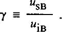
Each value of γ thus is linked directly to a value of K_s, and the calculations above require that γ « 1 (sliding velocity at UpB small compared to total velocity).

For τ* = 0 and N independent of z in Equation (8),Boulton and Hindmarsh (1987) determined empirically that a = 1.33, b = 1.8, and K_b = 2.8 χ 10⁻⁵Pa⁰⁴⁷S⁻¹ at Breidamerkurjökull. They did not report uncertainties, but we estimate standard errors of ±0.2–0.3 on the determination of a and b. We thus look for solutions with a and b within one to two standard errors of the Reference Boulton and HindmarshBoulton and Hindmarsh (1987) values. We focus on solutions with a = 1 because a = is mathematically simple, and because a = 1 falls within the likely error bounds from Reference Boulton and HindmarshBoulton and Hindmarsh (1987).

The till at Breidamerkurjökull is relatively coarsegrained compared to the tills beneath the Ross Sea used as a basis for our calculations (Reference BarrettBarrett, 1975; Reference Anderson, Kurtz, Domack and BaishawAnderson and others, 1980; Reference Boulton and HindmarshBoulton and Hindmarsh, 1987). Addition of clasts is known to strengthen earth flows in viscous deformation (Reference Rodine and JohnsonRodine and Johnson, 1976; Reference HamptonHampton, 1979). We thus expect K_b to be larger for Ice Stream B than for Breidamerkurjökull, but we do not know by how much.

Computationally, we estimate u _i T_b, d, and N along the idealized ice stream using β calculated at UpB. We then assume values for γ (and thus K_s), a, and b, and calculate u_s from Equation (7) and u_d from Equation (10). These results plus the assumed value of Z₁ allow us to calculate K_b from Equations (8) and (9) at each point along the idealized ice stream. Each set of (a, b, γ) yields a curve of K_b(x), but we argued above that K_b is likely to be independent of x. What we take as the “best fit” between model and real ice streams is that combination of (a, b, γ) that minimizes variation in K_b along the model ice stream and that meets the criteria of a, b within the error limits of Reference Boulton and HindmarshBoulton and Hindmarsh (1987), γ small, and K_b larger than for Breidamerkurjökull.

Results are shown in Figure 3, where we plot the maximum relative variation in K_b from χ = 100 km to χ = 300 km as a function of γ for different pairs of a and b. For instructional purposes, we deliberately have allowed a, b, and γ to vary past likely limits; only the (a, b) pairs (1.33, 1.8) and (1, 2) in Figure 3 fall within the likely error limits of Reference Boulton and HindmarshBoulton and Hindmarsh (1987), and only small γ are acceptable from Weertman-sliding calculations.

Fig. 3.

Relative variation in modeled till-softness parameter, K_b, as a function of y, the fraction of the ice velocity at UpB arising from sliding, for different parts of exponents (a, b) in Equation (8). The variation is given as , Where K _bmax and K _bmin are the maximum and minimum values of K_b, respectively, from x = 100 km (UpB) to x = 300km for given a, b, and γ. Curves for (a, b) = (1.33, 1.8), (I, 2), (1, 3), (1, 4), and (1, 5) are indicated; the heavy solid line connects the minima in Δ for a = 1, b = 2, 3, 4, 5.

It is evident that the BoulReference Boulton and Hindmarshton and Hindmarsh (1987) relation, a = 1.33, b = 1.8, gives a moderately good fit at small γ with an increase in K_b of about 12% down-stream. The absolute value of K_b (1.4 χ 10⁻³Pa^0.47S⁻¹) is higher than for Breidamerkurjökull (2.8 χ 10⁻⁵Pa^0.47S⁻¹), as expected.

A better fit is obtained for a = 1, b = 2, and small γ. Variation in K_b from x = 100 km to χ = 300 km (plotted in Figure 3) is minimized for γ ≈ 0 and amounts to only about 0.3%; variation from χ = 25 km to χ = 300 km is minimized for γ ≈ 0.05 and amounts to about 1% (see Fig. 4). For a = 1, b = 3, 4, 5, the value of γ that minimizes variation in K_b increases with increasing b (Fig. 3). The minimum variation in K_b also increases with b and the pattern of variation of K_b along the flow line becomes complicated (Fig. 4). Thus, models with b > 3 give a poor fit. In addition, b ≥ 3 falls outside of likely error bounds from Reference Boulton and HindmarshBoulton and Hindmarsh (1987) and large γ is unlikely based on calculations presented above, so these models are discarded.

Fig. 4.

Variation in modeled till-softness parameter, K_b, as a function of position, x, for different pairs of exponents (a, b) in Equation (8) and for different values of γ. The softness parameter, K_b, is plotted normalized by K_bmax, its maximum value for given (a, b) over all γ and x from 25 to 300 km. The values of (a, b) are indicated above each section of the figure. From top to bottom in each section, the curves are γ = 0, 0.1, 0.2..... 0.9. The most nearly horizontal curve in each section correponds to the best-fit value γ for (a, b) in that section.

We could conduct a formal inversion for those values of a, b, and γ that minimize variations in K_h along the model ice stream. However, it is clear from the results presented above that a ≈ 1, b ≈ 2, and γ ≈ 0–0.1 provide an excellent fit, with variation in K_b of ≤1% along the ice stream. Any improvement in this fit that might result from using decimal powers (e.g. b = 2.01) would not be statistically significant and would complicate the resulting flow law for till. We thus feel justified in using our simple forward approach to this inverse problem, and in taking a ≈ 1, b ≈ 2, and γ ≈ 0–0.1 as our best solution.

Sensitivity study and discussion of assumptions

The analysis above clearly is based on a number of assumptions. Most of these can be tested by surface geophysical and bore-hole studies of the ice-stream bed, and we expect such tests in the future. However, a complete data set is unlikely to be assembled for years, if ever. In the interim, the best we can do is to assess likely errors in assumed or inferred quantities, and to test how sensitive our results are to those errors.

The main inference, that bed deformation contributes a significant fraction of the total velocity of Ice Stream B (Reference Alley, Blankenship, Bentley and RooneyAlley and others, 1987b), is drawn from solid geophysical evidence (Blankenship and others, Reference Blankenship, Bentley, Rooney and Alley1987,1989; Rooney and others, Reference Rooney, Blankenship, Alley and Bentley1987b,1988). The alternative of a rigid or nearly rigid bed would require that the data or the inferences drawn from the data are in error. In addition, a rigid bed would require some combination of a smoother bed, thicker water layer, or error in the sliding law at UpB sufficient to allow the sliding velocity to be more than two orders of magnitude faster than calculated above, and to allow a further down-stream increase in sliding velocity not accounted for by modern sliding theory so that the error in sliding velocity calculated above approaches three orders of magnitude at the down-stream end. Although not impossible, we believe such errors to be unlikely, and we do not consider this possibility γ = 1) further.

However, it is possible that errors in sliding calculations are sufficiently large to allow significant sliding (and ploughing?) over a pervasively deforming bed (intermediate γ). Such a situation would not invalidate the inferences based on seismic data at UpB. It would require some ad hoc modifications in our assumed distribution of till roughness or softness along the ice stream. We now do not obtain good solutions for intermediate γ (see Fig. 4). Suppose that a = 1, b = 2, γ = 0.3 (which requires that sliding has been underestimated by a factor of 45 at UpB). Then an exact fit with constant K_s would require K_b to vary as shown in Figure 4 in the (1, 2) section for the y = 0.3 curve (fourth from the top); that is, a slight decrease followed by a 32% increase in the down-stream direction.

The calculation of effective pressure, N, used the geometric factor β from Equation (6), which we calculated using the seismically estimated effective pressure of 50 ± 40 kPa at UpB (Reference Blankenship, Bentley, Rooney and AlleyBlankenship and others, 1987). The error limits on N produce a corresponding error in β (β = 2.1 ± 1.6). However, an error in β means only that all estimates of N along the flow line are in error by a constant multiplicative factor of between 0.2 and 1.8, and thus that our estimate of K_b for any chosen (a, b, y) will be in error by that multiplicative factor raised to the power b. The only restriction we could place on K_b was that it exceed the value calculated for Breidamerkurjökull (Reference Boulton and HindmarshBoulton and Hindmarsh, 1987), which it does for the full range of ß = 2.1 ± 1.6. Thus, errors in β have no significant effect on our result.

The assumption of constant deforming-layer thickness, z_v does affect the result significantly. The thickness at UpB is relatively well determined seismically at about 6 m (Reference Rooney, Blankenship, Alley and BentleyRooney and others, 1987b), but there is more uncertainty in our knowledge of Z₁ at the down-stream end (Reference Blankenship, Rooney, Alley and BentleyBlankenship and others, 1989). Suppose we let Z₁ = 6 ± 3 m at the down-stream end, z_χ = 6 m at UpB, and we assume that Z₁ varies linearly along the ice stream. If we further assume that a = 1, then we can assess the impact of errors in Z₁ on b. The best fit for a 9 m thick deforming layer at the down-stream end with a = 1 is b ≈ 1, γ ≈ 0, whereas for 3 m thick till there it is b ≈ 3, γ ≈ 0.

This result is relatively easy to understand. The shear stress decreases down-stream, but the sliding velocity remains low and is calculated to decrease down-stream from UpB. At the same time, the total velocity increases downstream. With constant K_b, the down-stream increase in velocity must arise from thicker or softer till down-stream. The effective pressure, N, decreases down-stream and causes the till to soften down-stream. If the till thins down-stream, then the inverse dependence of softness on N must be strong (large b), whereas if the till thickens down-stream, this dependence can be weak (small b).

Another important assumption is that of N independent of z. It is not difficult to show that allowing N to increase with depth in till will increase the value of b in the best-fit result by an additive factor of zero to one, as compared to the case of depth-independent N.

To see this, return to the coordinate system of part II, with z = 0 at the ice-till interface, positive downward. Set τ* = 0 in Equation (8), take T_b and N to be independent of z₁ and let u = u₀ at z = 0 and u = 0 at z = z_v Then, integrating Equation (8) through the till thickness and solving for K_b yields

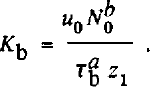
The variation of effective pressure with depth can be written (part II, equation (17))

where N₀ is the effective pressure at z = 0 (the ice—bed interface), Δp is the difference between the bulk density and the pore-fluid density, and g is the gravitational acceleration. (If downward water flow to an aquifer were to occur, then N would increase with depth more rapidly than given by Equation (13). This could be modeled by defining where p_b and ρ_ω are the bulk and water densities, respectively, and H is the hydraulic head. The assumption of no vertical water flow is equivalent to assuming H independent of z.) Substituting Equation (13) into Equation (8) with τ* = 0, integrating through the thickness, and solving for the softness coefficient yields

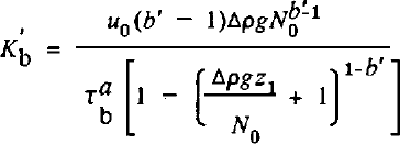
where primed quantities refer to the case of depth-varying N. (Equation (14) is valid only for b ≠ 1; a similar expression with logarithmic terms arises for b = 1. We generally expect b > 1, and so do not display this.)

Two limits bear consideration in Equation (14). If Δpgz₁ « N₀ (variation in effective pressure across layer small compared to effective pressure at the top), then Equation (14) reduces to Equation (12) and b' = b. If Δpgz₁ » N₀ (variation in effective pressure across layer large compared to effective pressure at top) then Equation (14) reduces to

Because Δρ, g, b', and Z₁ are constants in any experiment, Equation (15) shows that the best fit is obtained for b' = b + I. Thus, if (a,b, γ) ≈ (1,2,0–0.1) for depth-independent effective pressure, we expect the same result if effective pressure varies with depth but Δpgz₁ « N₀, and we expect (1,3,0–0.1 if Δpgz₁ » N_Q ; the complete range of possibilities is spanned by (1,2–3,0–0.1).

Near the UpB camp, seismic measurements give N = 50 ± 40 kPa averaged over a local till thickness of 8 m (Reference Blankenship, Bentley, Rooney and AlleyBlankenship and others, 1987). (The average till thickness near UpB is 6 m, but there are local variations (Reference Rooney, Blankenship, Alley and BentleyRooney and others, 1987b).) Ice Stream B is unlikely to experience significant vertical drainage into subglacial aquifers (Reference Linge and BrownLingle and Brown, 1987; also see above and part I), meaning that the depth variation of pressure is limited by the lithostatic (Δρ = 0) and hydrostatic (Δρ * 10^s kg m⁻³) cases (part II, equations (17) and (18)). In the hydrostatic case, N varies vertically by about 10 kPa/m. If we assume that N = 50 ± 40 kPa applies to the center of the till at ζ = 4 m at UpB, and that the hydrostatic case applies, then N₀ = 10 ± 40 kPa. Physically, N₀ ≤ 0 cannot occur over large areas because it would imply floating ice and zero basal shear stress, whereas a non-zero basal shear stress exists. We thus take 0 > N₀ ≤ 50 kPa in the hydrostatic case.

For till averaging Z₁ = 6 m thick with a hydrostatic pressure gradient, Apgz₁ ≈ 60 kPa. If W₀ ≈ 0, then Apgz₁ » N₀ and we expect b ≈ 3 3; however, if N₀ ≈ 50 kPa, then Apgz₁ ≈ N₀ and we expect b between 2 and 3. Computer simulations give b = 3.0 for Af₀ ≈ 0 and b = 2.7 for N₀ = 50 kPa, as expected.

The assumptions τ* = 0 (no yield strength) proves to affect the results mainly through its control on the deforming thickness, provided that cohesion is small. If N is independent of depth, then

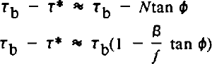
from equation (22) in part II with cohesion set to zero, and from Equation (6). The fraction of the bed flooded, f, varies only slowly along flow, and β and tan φ are constants. Thus, τ* is approximately a constant multiplied by T_b, and τ – τ* is a different constant multiplied by T_b. The resulting (a,b,y) are essentially the same as the τ*= 0 case, but with the magnitude of K_b changed slightly, giving (a,b,y) ≈ (1,2,0–0.1) for cohesionless till with non-zero internal friction and depth-independent effective pressure.

If we allow cohesion and increase of effective pressure with depth, then Equation (16) becomes

The effect of choosing some combination of Δρ, tan φ, and C such that τ* is as large as possible without reducing the deforming thickness below 6 m anywhere along the flow line (i.e. without making τ* > T_b at Z₁ = 6 m) is to increase b to about 3 for a = 1, but with y = 0–0.1 still. Smaller τ* reduces b back toward 2, and larger τ* reduces the deforming thickness down-stream and increases b to about 4 for a 3 m till at the down-stream end.

We have assumed that all of the ice velocity arises from sliding and pervasive till deformation. Clearly, if some additional deformational mechanisms are active, this assumption could introduce errors. Possible candidates include ploughing and shearing on discrete planes.

Ploughing was defined for motion over a rigid bed (Reference Brown, Hallet and BoothBrown and others, 1987), but one can conceive of accelerated motion of some clasts through a bed undergoing slow pervasive deformation. Unless there are quite steep vertical gradients in effective viscosity, however, our calculations (see “ploughing” in part II) suggest that such localized velocity is unlikely to be large. Large ploughing velocities were not reported at Breidamerkurjökull (Reference BoultonBoulton, 1979) or Blue Glacier (Reference Engelhardt, Harrison and KambEngelhardt and others, 1978) (see “ploughing”, part II). It thus seems quite reasonable to partition the velocity near the ice—till interface to sliding and pervasive deformation only.

Discrete shear at the base of the till is more problematic. Reference Boulton and HindmarshBoulton and Hindmarsh (1987) found that at Breidamerkurjökull, where a pervasively deforming till overlies a lodged till that differs from it only in ways related directly to the deformation, a significant fraction (10–30%) of the total deformational velocity arises from shearing on discrete surfaces in the deeper layer (see section on “velocity-depth profiles”, part II). We could introduce an explicit relation for velocities from discrete shearing. The total velocity would increase with shear stress and with the inverse of effective pressure, the same as for pervasive deformation, but the form of the relation is poorly constrained. Implicitly treating discrete shearing as part of pervasive deformation may be as accurate as any other approach, especially considering that discrete shearing seems unlikely to be the dominant contributor to basal velocity. We thus feel justified in not treating discrete shearing explicitly; below we discuss whether such shearing is likely beneath Ice Stream B.

To recapitulate, we assume that the basal system of Ice Stream B obeys Equations (1)—( 10), and that the grain-size distribution controls the geometric factors K_s, K_b, and β, and does not vary along flow. The longitudinal profile of the ice stream, as idealized in Figure 1, then requires that b ≈ 2, γ ≈ 0–0.1 for a = 1 in Equation (8), if τ* = 0 and N is independent of depth in the till and if the deforming till thickness is constant along the ice stream. Allowing N to vary with depth in the till increases b to between 2 and 3. Allowing τ* to be significant but setting the cohesion to zero has little effect on b; increasing the cohesion acts with depth-varying N to increase b toward 3. If the deforming till thickness varies, owing to the effect of T* or to a lithologie change, then b also varies; a 3 m thickening from UpB to the down-stream end reduces b by about 1, and a 3 m thinning from UpB to the down-stream end increases b by about 1.