1 Introduction
The systematic investigation of particles at low Reynolds number involving both analytical and numerical studies traces back to the work of Brenner (Reference Brenner1963, Reference Brenner1964) and O’Neill (Reference O’Neill1968, Reference O’Neill1969), which have provided a comprehensive review of the literature and various techniques for viscous flow containing solid particles. Stokes flow with more particles was analytically analysed by Mazur & van Saarloos (Reference Mazur and van Saarloos1982) and Kim (Reference Kim1987), and numerically analysed by Wilson (Reference Wilson2013). The presence of a boundary significantly affects the flow behaviour (Shen, Marcos & Fu Reference Shen and Fu2017). A large body of literature has considered flow behaviour with boundary effect, including the general solutions under different background flows (Lamb & Caflisch Reference Lamb and Caflisch1993) and extra forces acting on the fluid (Marcos et al. Reference Kang, Ooi, Yang and Wong2005a ,Reference Ooi, Yang, Chai and Wong b ; Feng et al. Reference Feng, Wong and Che2016; Huang et al. Reference Huang, Chen, Wong and Liow2016; Huang, Wang & Wong Reference Huang, Wang and Wong2017). One typical example of a commonly encountered boundary is a cylindrical tube. The motion of small particles in a cylindrical tube at low Reynolds number is of importance to many fields, such as drug delivery through blood capillaries, lubrication theory, microfluidic and nanofluidic applications in biotechnology and chemical reaction engineering (Ho & Tai Reference Ho and Tai1998; Bhattacharya, Mishra & Bhattacharya Reference Bhattacharya, Mishra and Bhattacharya2010; Koh & Marcos Reference Koh2014; Marcos et al. Reference Tran, Saini, Ong and Chia2014). The motion of a single particle travelling in a cylindrical tube had been investigated by Brenner & Happel (Reference Brenner and Happel1958), Greenstein & Happel (Reference Greenstein and Happel1968), Hasimoto (Reference Hasimoto1976) and Bhattacharya et al. (Reference Bhattacharya, Mishra and Bhattacharya2010). When there are two or more particles travelling in the tube, the flow field is more complex due to particle–particle interaction (Zhong & Duan Reference Zhong and Duan2016; Zhong, Xie & Duan Reference Zhong, Xie and Duan2017). The motion of two or more spherical particles translating along the axis of the tube has been investigated by Sonshine & Brenner (Reference Sonshine and Brenner1966), Wang & Skalak (Reference Wang and Skalak1969), Leichtberg, Pfeffer & Weinbaum (Reference Leichtberg, Pfeffer and Weinbaum1976) and spheroidal particles by Chen & Skalak (Reference Chen and Skalak1970). Navardi & Bhattacharya (Reference Navardi and Bhattacharya2013) calculated the hydrodynamic forces on two particles travelling in a cylindrical tube. The drag force and torque tensors were obtained. A related result using the same methodology was presented by Navardi, Bhattacharya & Wu (Reference Navardi, Bhattacharya and Wu2015), who gave the Stokesian simulation of two particles freely moving in a cylinder.
The flow field around a moving porous particle depends on its permeability.
When the particle has zero permeability, the fluid has to travel around the
particle. When the permeability is non-zero, the fluid can pass through the
particle. Many materials, such as agarose and hydrogel, are highly permeable.
They are typically used as a membrane for separation devices (Kapur
et al.
Reference Kapur, Charkoudian, Kessler and Anderson1996; Mika & Childs Reference Mika and Childs2001; Buehler & Anderson Reference Buehler and Anderson2002). Agarose has also been fabricated in
nanoscale or microscale for bioengineering and energy storage applications
(Chudasama, Prasad & Siddhanta Reference Chudasama, Prasad and Siddhanta2016; Kim et al.
Reference Kim, Koo, Liu and Braun2017). Permeable particles could be
modelled as porous materials. The flow within the porous region can be
described using the Darcy equation or the Brinkman equation while the flow of
the fluid in the cylinder is governed by the steady-state Stokes equation.
Darcy’s law states that the fluid flow is linearly proportional to the pressure
gradient and the gravitational force (Mokadam Reference Mokadam1961). However, the Darcy equation is not compatible with the
existence of a boundary layer region (Beavers & Joseph Reference Beavers and Joseph1967; Neale & Nader Reference Neale and Nader1974). The Brinkman equation, however, has
been found to be consistent with the predictions made by applying Darcy’s law
without the need to resort to empirical boundary conditions. The validity of
the Brinkman equation has been extensively treated in the literature (Nield
& Bejan Reference Nield and Bejan2006). Though there are
several limitations, the Brinkman equation with continuity of velocity and
normal stress at the porous interface is believed to be a successful model of
steady Stokes flow past highly permeable particles (Prakash & Sekhar
Reference Prakash and Sekhar2012). Higdon & Kojima (Reference Higdon and Kojima1981) derived asymptotic results for Stokes
flow passing porous particles of large and small permeability with arbitrary
geometry using the Brinkman equation. Padmavathi, Amaranath & Nigam
(Reference Padmavathi, Amaranath and Nigam1993) derived a solution for
non-axisymmetric Stokes flow passing through a stationary porous sphere. Neale,
Epstein & Nader (Reference Neale, Epstein and Nader1973) discussed
various possible solutions to the problem of unbounded creeping flow passing
through a porous sphere and generalized the solution to cover a swarm of
spheres. Vainshtein, Shapiro & Gutfinger (Reference Vainshtein, Shapiro and Gutfinger2002) examined the flow around and within an isolated
porous spheroid. Mo & Sangani (Reference Mo and Sangani1994) proposed a method to compute Stokes flow interactions among
spherical objects, including the case for
 $N$
porous particles within a periodic cubic unit cell.
Studies of porous particles translating in a cylindrical channel have been more limited. Saad & Faltas (Reference Saad and Faltas2014) solved the flow of a single porous particle in a cylindrical channel using an analytical–numerical method, constructing a general solution from the superposition of the fundamental solutions in both cylindrical and spherical coordinate systems and solving the boundary conditions using a collocation technique. There seems to be no literature on the solution to the problem of creeping flow passing and within two or more porous spherical particles translating in a cylinder.
This paper details a semi-analytical approach to solve for the flow of two freely translating porous particles in a viscous fluid along the axis of a cylindrical tube. The flows inside and outside the porous particles are governed by the Brinkman equation and the Stokes equation, respectively. The fluid passing through the porous material will induce drag forces acting on the two particles. The calculation is performed in an iterated framework using the method of reflections. We analyse the hydrodynamic forces and velocities of the two particles, which are dependent on the distance between the two particles and particle sizes. This information can give a better understanding of the interaction between porous particles.
2 Problem statement
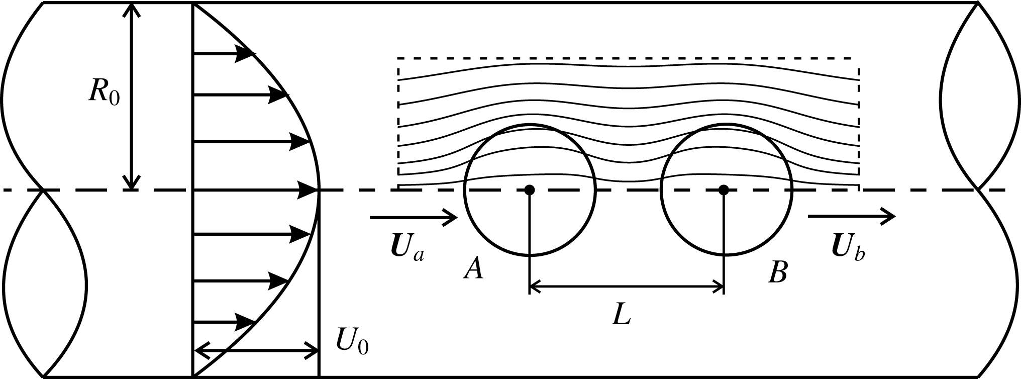
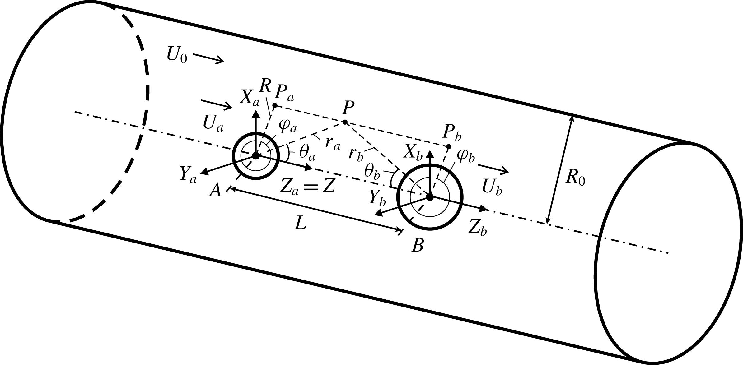
We consider two porous spherical particles translating freely along the axis of
a cylindrical tube of radius
 $R_{0}$
with a background Poiseuille flow at low Reynolds number
(figure 1). In this model,
 $(R,\unicode[STIX]{x1D6F7},Z)$
, giving the radial distance, azimuthal angle, axial distance,
represents the cylindrical coordinates with the
 $Z$
-axis coinciding with the tube axis while
 $(r_{a(b)},\unicode[STIX]{x1D703}_{a(b)},\unicode[STIX]{x1D711}_{a(b)})$
, giving the radial distance, polar angle, azimuthal angle,
are the spherical coordinates distinguished by appending the subscripts
 $a$
and
 $b$
with their corresponding origins at the centres of particle
 $A$
and particle
 $B$
, respectively.
 $L$
is the separation distance between the centres of particles
 $A$
and
 $B$
along the axis of the cylinder. Due to the relative positions
of the two spheres along the axis (axisymmetric configuration) and the uniform
permeability, each particle only has a translational velocity
 $\boldsymbol{U}$
along the
 $Z$
-direction with subscripts
 $a$
and
 $b$
corresponding to particle
 $A$
and particle
 $B$
, respectively. In this section, we outline the governing
equations and boundary conditions involved, and the procedures to approach this
problem.
Schematics of two porous spheres translating along the axis of a
cylindrical tube with radius
 $R_{0}$
. Two spheres,
 $A$
and
 $B$
, with radii
 $a$
and
 $b$
, respectively, are placed along the axis of the
tube. The background flow field of the cylinder has a parabolic
profile with the maximum velocity
 $U_{0}$
at the axis.
 $L$
is the separation distance between the centres of
spheres
 $A$
and
 $B$
.

2.1 Governing equations and boundary conditions
The flow field around the moving porous particles depends on their
permeability. When the two particles are impermeable (zero permeability),
the fluid has to travel around the particles. If the permeability is
non-zero, the fluid can pass through the two particles (region marked in
figure 1 with a dashed rectangle).
In such a case, at low Reynolds number, the governing equations for the
model are the Stokes equation for the external steady Newtonian fluid flow
outside the particles (
 $r_{a}>a$
,
 $r_{b}>b$
) and the Brinkman equation for the internal porous region (
 $0<r_{a}<a$
,
 $0<r_{b}<b$
):
 $$\begin{eqnarray}\displaystyle & \displaystyle \unicode[STIX]{x1D6FB}^{2}\boldsymbol{v}^{e}=\frac{1}{\unicode[STIX]{x1D707}}\unicode[STIX]{x1D735}p^{e},\quad \unicode[STIX]{x1D735}\boldsymbol{\cdot }\boldsymbol{v}^{e}=0, & \displaystyle\end{eqnarray}$$
 $$\begin{eqnarray}\displaystyle & \displaystyle \unicode[STIX]{x1D6FB}^{2}\boldsymbol{v}^{i}=\frac{1}{\unicode[STIX]{x1D707}}\unicode[STIX]{x1D735}p^{i}+\frac{1}{k}\boldsymbol{v}^{i},\quad \unicode[STIX]{x1D735}\boldsymbol{\cdot }\boldsymbol{v}^{i}=0, & \displaystyle\end{eqnarray}$$
where
 $\unicode[STIX]{x1D707}$
is the viscosity of the fluid and
 $k$
is the permeability of the porous material. The
superscripts ‘
 $e$
’ and ‘
 $i$
’ represent the external and internal flows of the porous
particles, respectively. The flow field
 $\boldsymbol{v}$
and induced stress tensors components
 $\unicode[STIX]{x1D635}_{rr}$
and
 $\unicode[STIX]{x1D635}_{r\unicode[STIX]{x1D703}}$
are continuous at the fluid-particle interface. The
boundary conditions are
 $$\begin{eqnarray}\displaystyle & (\boldsymbol{v}^{e}-\boldsymbol{U})\boldsymbol{\cdot }\boldsymbol{n}=\boldsymbol{v}^{i}\boldsymbol{\cdot }\boldsymbol{n}, & \displaystyle\end{eqnarray}$$
 $$\begin{eqnarray}\displaystyle & (\boldsymbol{v}^{e}-\boldsymbol{U})\boldsymbol{\cdot }\boldsymbol{s}=\boldsymbol{v}^{i}\boldsymbol{\cdot }\boldsymbol{s}, & \displaystyle\end{eqnarray}$$
 $$\begin{eqnarray}\displaystyle & \unicode[STIX]{x1D635}_{rr}^{e}=\unicode[STIX]{x1D635}_{rr}^{i}, & \displaystyle\end{eqnarray}$$
 $$\begin{eqnarray}\displaystyle & \unicode[STIX]{x1D635}_{r\unicode[STIX]{x1D703}}^{e}=\unicode[STIX]{x1D635}_{r\unicode[STIX]{x1D703}}^{i}, & \displaystyle\end{eqnarray}$$
where
 $\boldsymbol{n}$
is the unit vector normal to the porous-fluid interface
and pointing to the external fluid and
 $\boldsymbol{s}$
is the tangential vector at the interface. It should be
noted that
 $\boldsymbol{v}^{i}$
represents the relative velocity of the fluid inside the
porous particle with respect to the origin of the particle and
 $\boldsymbol{v}^{e}$
refers to the velocity in an inertial reference frame.
Therefore, the particle velocity must be subtracted from
 $\boldsymbol{v}^{e}$
to construct the boundary conditions (2.3)–(2.4). On the wall of the
cylindrical tube, the no-slip boundary condition applies:
 $$\begin{eqnarray}\boldsymbol{v}^{e}=0.\end{eqnarray}$$
2.2 Semi-analytical implementation
2.2.1 Calculation procedure based on the method of reflections
Since the governing equations and boundary conditions are linear, the velocity and pressure fields can be expressed as a summation of fields:
 $$\begin{eqnarray}\displaystyle & \boldsymbol{v}=\boldsymbol{v}_{c}^{(0)}+\boldsymbol{v}_{a}^{(1)}+\boldsymbol{v}_{b}^{(2)}+\boldsymbol{v}_{c}^{(3)}+\boldsymbol{v}_{a}^{(4)}+\boldsymbol{v}_{b}^{(5)}+\cdots , & \displaystyle\end{eqnarray}$$
 $$\begin{eqnarray}\displaystyle & p=p_{c}^{(0)}+p_{a}^{(1)}+p_{b}^{(2)}+p_{c}^{(3)}+p_{a}^{(4)}+p_{b}^{(5)}+\cdots , & \displaystyle\end{eqnarray}$$
where the superscript (
 $j$
) refers to the
 $j$
th reflection (
 $j=1,2,3\ldots$
) and subscripts
 $a$
,
 $b$
and
 $c$
refer to the boundary conditions satisfying particle
 $A$
, particle
 $B$
and the cylinder, respectively. Each term of
 $\boldsymbol{v}$
and
 $p$
separately satisfies the governing equations (2.1)–(2.2) and the boundary
conditions resulting from the previous terms. For example, if the
subscript of the last term is
 $b$
, the summation of the terms satisfies the boundary
condition of particle
 $B$
. It should be noted that the reflections representing
the flow fields due to the porous particles (reflections with subscripts ‘
 $a$
’ and ‘
 $b$
’) consist of two components: the flows inside and
outside the porous particles with superscripts ‘
 $i$
’ and ‘
 $e$
’, respectively. Therefore, equation (2.8) becomes
 $$\begin{eqnarray}\displaystyle & \boldsymbol{v}^{e}=\boldsymbol{v}_{c}^{(0)}+\boldsymbol{v}_{a}^{(1,e)}+\boldsymbol{v}_{b}^{(2,e)}+\boldsymbol{v}_{c}^{(3)}+\boldsymbol{v}_{a}^{(4,e)}+\boldsymbol{v}_{b}^{(5,e)}+\cdots , & \displaystyle\end{eqnarray}$$
 $$\begin{eqnarray}\displaystyle & \boldsymbol{v}_{a}^{i}=\boldsymbol{v}_{a}^{(1,i)}+\boldsymbol{v}_{a}^{(4,i)}+\boldsymbol{v}_{a}^{(7,i)}+\cdots , & \displaystyle\end{eqnarray}$$
 $$\begin{eqnarray}\displaystyle & \boldsymbol{v}_{b}^{i}=\boldsymbol{v}_{b}^{(2,i)}+\boldsymbol{v}_{b}^{(5,i)}+\boldsymbol{v}_{b}^{(8,i)}+\cdots . & \displaystyle\end{eqnarray}$$
Based on the boundary conditions (2.3)–(2.6), the following relations can be obtained:
 $$\begin{eqnarray}\displaystyle & \boldsymbol{v}_{c}^{(0)}=[U_{0}(1-R^{2}/R_{0}^{2})]\boldsymbol{Z}, & \displaystyle\end{eqnarray}$$
 $$\begin{eqnarray}\displaystyle & \boldsymbol{v}_{a}^{(1)}=\left\{\begin{array}{@{}ll@{}}(\boldsymbol{v}_{a}^{(1,e)}+\boldsymbol{v}_{c}^{(0)}-\boldsymbol{U}_{a})\boldsymbol{\cdot }\boldsymbol{n}=\boldsymbol{v}_{a}^{(1,i)}\boldsymbol{\cdot }\boldsymbol{n}, & \text{at}~r_{a}=a,\\ (\boldsymbol{v}_{a}^{(1,e)}+\boldsymbol{v}_{c}^{(0)}-\boldsymbol{U}_{a})\boldsymbol{\cdot }\boldsymbol{s}=\boldsymbol{v}_{a}^{(1,i)}\boldsymbol{\cdot }\boldsymbol{s}, & \text{at}~r_{a}=a,\\ \unicode[STIX]{x1D635}_{a,rr}^{(1,e)}=\unicode[STIX]{x1D635}_{a,rr}^{(1,i)}, & \text{at}~r_{a}=a,\\ \unicode[STIX]{x1D635}_{a,r\unicode[STIX]{x1D703}}^{(1,e)}=\unicode[STIX]{x1D635}_{a,r\unicode[STIX]{x1D703}}^{(1,i)}, & \text{at}~r_{a}=a,\\ 0, & \text{at}~Z=\pm \infty ,\end{array}\right. & \displaystyle\end{eqnarray}$$
 $$\begin{eqnarray}\displaystyle & \boldsymbol{v}_{b}^{(2)}=\left\{\begin{array}{@{}ll@{}}(\boldsymbol{v}_{b}^{(2,e)}+\boldsymbol{v}_{a}^{(1,e)}+\boldsymbol{v}_{c}^{(0)}-\boldsymbol{U}_{b})\boldsymbol{\cdot }\boldsymbol{n}=\boldsymbol{v}_{b}^{(2,i)}\boldsymbol{\cdot }\boldsymbol{n}, & \text{at}~r_{b}=b,\\ (\boldsymbol{v}_{b}^{(2,e)}+\boldsymbol{v}_{a}^{(1,e)}+\boldsymbol{v}_{c}^{(0)}-\boldsymbol{U}_{b})\boldsymbol{\cdot }\boldsymbol{s}=\boldsymbol{v}_{b}^{(2,i)}\boldsymbol{\cdot }\boldsymbol{s}, & \text{at}~r_{b}=b,\\ \unicode[STIX]{x1D635}_{b,rr}^{(2,e)}=\unicode[STIX]{x1D635}_{b,rr}^{(2,i)}, & \text{at}~r_{b}=b,\\ \unicode[STIX]{x1D635}_{b,r\unicode[STIX]{x1D703}}^{(2,e)}=\unicode[STIX]{x1D635}_{b,r\unicode[STIX]{x1D703}}^{(2,i)}, & \text{at}~r_{b}=b,\\ 0, & \text{at}~Z=\pm \infty ,\end{array}\right. & \displaystyle\end{eqnarray}$$
 $$\begin{eqnarray}\displaystyle & \boldsymbol{v}_{c}^{(3)}=\left\{\begin{array}{@{}ll@{}}-\boldsymbol{v}_{a}^{(1,e)}-\boldsymbol{v}_{b}^{(2,e)}, & \text{at}~R=R_{0},\\ 0, & \text{at}~Z=\pm \infty ,\end{array}\right. & \displaystyle\end{eqnarray}$$
 $$\begin{eqnarray}\displaystyle & \boldsymbol{v}_{a}^{(4)}=\left\{\begin{array}{@{}ll@{}}(\boldsymbol{v}_{a}^{(4,e)}+\boldsymbol{v}_{b}^{(2,e)}+\boldsymbol{v}_{c}^{(3)})\boldsymbol{\cdot }\boldsymbol{n}=\boldsymbol{v}_{a}^{(4,i)}\boldsymbol{\cdot }\boldsymbol{n}, & \text{at}~r_{a}=a,\\ (\boldsymbol{v}_{a}^{(4,e)}+\boldsymbol{v}_{b}^{(2,e)}+\boldsymbol{v}_{c}^{(3)})\boldsymbol{\cdot }\boldsymbol{s}=\boldsymbol{v}_{a}^{(4,i)}\boldsymbol{\cdot }\boldsymbol{s}, & \text{at}~r_{a}=a,\\ \unicode[STIX]{x1D635}_{a,rr}^{(4,e)}=\unicode[STIX]{x1D635}_{a,rr}^{(4,i)}, & \text{at}~r_{a}=a,\\ \unicode[STIX]{x1D635}_{a,r\unicode[STIX]{x1D703}}^{(4,e)}=\unicode[STIX]{x1D635}_{a,r\unicode[STIX]{x1D703}}^{(4,i)}, & \text{at}~r_{a}=a,\\ 0, & \text{at}~Z=\pm \infty ,\end{array}\right. & \displaystyle\end{eqnarray}$$
 $$\begin{eqnarray}\displaystyle & \boldsymbol{v}_{b}^{(5)}=\left\{\begin{array}{@{}ll@{}}(\boldsymbol{v}_{b}^{(5,e)}+\boldsymbol{v}_{a}^{(4,e)}+\boldsymbol{v}_{c}^{(3)})\boldsymbol{\cdot }\boldsymbol{n}=\boldsymbol{v}_{a}^{(5,i)}\boldsymbol{\cdot }\boldsymbol{n}, & \text{at}~r_{b}=b,\\ (\boldsymbol{v}_{b}^{(5,e)}+\boldsymbol{v}_{a}^{(4,e)}+\boldsymbol{v}_{c}^{(3)})\boldsymbol{\cdot }\boldsymbol{s}=\boldsymbol{v}_{a}^{(5,i)}\boldsymbol{\cdot }\boldsymbol{s}, & \text{at}~r_{b}=b,\\ \unicode[STIX]{x1D635}_{b,rr}^{(5,e)}=\unicode[STIX]{x1D635}_{b,rr}^{(5,i)}, & \text{at}~r_{b}=b,\\ \unicode[STIX]{x1D635}_{b,r\unicode[STIX]{x1D703}}^{(5,e)}=\unicode[STIX]{x1D635}_{b,r\unicode[STIX]{x1D703}}^{(5,i)}, & \text{at}~r_{b}=b,\\ 0, & \text{at}~Z=\pm \infty ,\end{array}\right. & \displaystyle\end{eqnarray}$$
 $$\begin{eqnarray}\vdots\end{eqnarray}$$
For illustration, the calculation is conducted from the background flow
having a parabolic profile,
 $\boldsymbol{v}_{c}^{(0)}$
. The following reflection,
 $\boldsymbol{v}_{a}^{(1)}$
, due to the presence of particle
 $A$
, is required to make the summation
 $\boldsymbol{v}_{c}^{(0)}+\boldsymbol{v}_{a}^{(1)}$
satisfy the boundary condition of particle
 $A$
(as shown in (2.3)–(2.6)).
To acquire the boundary condition of
 $\boldsymbol{v}_{a}^{(1)}$
, we transform the expression of
 $\boldsymbol{v}_{c}^{(0)}$
in the cylindrical coordinates into the spherical
coordinates (details of the coordinate transformation are provided in
appendix A). The expression of
 $\boldsymbol{v}_{a}^{(1)}$
can be calculated by means of a stream function, which
will be described in § 2.2.2.
Similarly, the following reflection
 $\boldsymbol{v}_{b}^{(2)}$
is included to make the summation
 $\boldsymbol{v}_{c}^{(0)}+\boldsymbol{v}_{a}^{(1)}+\boldsymbol{v}_{b}^{(2)}$
satisfy the boundary condition of particle
 $B$
. The expression can be solved using a similar procedure
in the spherical coordinates of particle
 $B$
. The added reflection
 $\boldsymbol{v}_{c}^{(3)}$
is needed to make the summation satisfy the boundary
condition of the tube. The expressions derived in spherical coordinates
of particle
 $A$
,
 $\boldsymbol{v}_{a}^{(1)}$
, and particle
 $B$
,
 $\boldsymbol{v}_{b}^{(2)}$
, should be transformed into cylindrical coordinates,
such that
 $\boldsymbol{v}_{c}^{(3)}$
can be solved by utilizing cylindrical harmonics shown
in § 2.2.3.
In general, the reflection
 $\boldsymbol{v}_{a}^{(1)}$
arising from
 $\boldsymbol{v}_{c}^{(0)}$
brings in the representative geometry dimensions
 $a$
(the radius of particle
 $A$
) and
 $R_{0}$
(the radius of the tube) included in the form
 $a/R_{0}$
by using a stream function. This indicates that the
error at least scales as
 $a/R_{0}$
(Kim & Karrila Reference Kim and Karrila2005). The next reflection
 $\boldsymbol{v}_{b}^{(2)}$
is calculated from
 $\boldsymbol{v}_{a}^{(1)}$
and
 $\boldsymbol{v}_{c}^{(0)}$
. The velocity field introduces the term
 $b/R_{0}$
and
 $b/L$
, where
 $L$
is the separation distance between the two particles.
This indicates that the error at least scales as the maximum value of
 $b/R_{0}$
and
 $b/L$
. The following reflection
 $\boldsymbol{v}_{c}^{(3)}$
is required to satisfy the boundary condition:
 $\boldsymbol{v}_{c}^{(3)}=-\boldsymbol{v}_{a}^{(1)}-\boldsymbol{v}_{b}^{(2)}$
at the cylinder wall. The magnitude of
 $\boldsymbol{v}_{c}^{(3)}$
scales as the same order of
 $\boldsymbol{v}_{a}^{(1)}$
and
 $\boldsymbol{v}_{b}^{(2)}$
at the wall, which is smaller than that near
 $\boldsymbol{v}_{a}^{(1)}$
and
 $\boldsymbol{v}_{b}^{(2)}$
. This indicates the error of
 $\boldsymbol{v}_{c}^{(3)}$
is smaller than the error of
 $\boldsymbol{v}_{a}^{(1)}$
and
 $\boldsymbol{v}_{b}^{(2)}$
. Therefore, the subsequent reflection can correct the
error of the flow field to the higher order. By repeating the procedures
and adding more reflections, the results are expected to converge. This
convergence is verified in all our calculations (see appendix B).
2.2.2 Solution based on stream function
The solution of the external and internal flows of the porous particle in spherical coordinates can be expressed using the stream functions (Saad & Faltas Reference Saad and Faltas2014)
 $$\begin{eqnarray}\displaystyle & \displaystyle \unicode[STIX]{x1D6F7}^{e}=\mathop{\sum }_{n=2}^{\infty }(A_{n}r^{-n+1}+B_{n}r^{-n+3})C_{n}(\cos \unicode[STIX]{x1D703}), & \displaystyle\end{eqnarray}$$
 $$\begin{eqnarray}\displaystyle & \displaystyle \unicode[STIX]{x1D6F7}^{i}=\mathop{\sum }_{n=2}^{\infty }(\tilde{A}_{n}r^{n}+\sqrt{r}\tilde{B}_{n}I_{n-1/2}(\unicode[STIX]{x1D6FC}r))C_{n}(\cos \unicode[STIX]{x1D703}), & \displaystyle\end{eqnarray}$$
where
 $\unicode[STIX]{x1D6FC}=\sqrt{1/k}$
;
 $I_{n-1/2}$
is the modified Bessel function of the first kind;
 $C_{n}$
is the Gegenbauer polynomial of the first kind of order
 $n$
and degree
 $-1/2$
;
 $A_{n}$
,
 $B_{n}$
,
 $\tilde{A}_{n}$
and
 $\tilde{B}_{n}$
are unknown coefficients which can be determined from
the boundary conditions as shown in (2.3)–(2.6).
The velocity components in spherical coordinates can be derived from the stream functions
 $$\begin{eqnarray}\displaystyle & \displaystyle v_{r}^{e,i}=-\frac{1}{r^{2}\sin \unicode[STIX]{x1D703}}\frac{\unicode[STIX]{x2202}\unicode[STIX]{x1D6F7}^{e,i}}{\unicode[STIX]{x2202}\unicode[STIX]{x1D703}}, & \displaystyle\end{eqnarray}$$
 $$\begin{eqnarray}\displaystyle & \displaystyle v_{\unicode[STIX]{x1D703}}^{e,i}=\frac{1}{r\sin \unicode[STIX]{x1D703}}\frac{\unicode[STIX]{x2202}\unicode[STIX]{x1D6F7}^{e,i}}{\unicode[STIX]{x2202}r}, & \displaystyle\end{eqnarray}$$
By substituting (2.19)–(2.20) into (2.21)–(2.22), the velocity components can be expressed as
 $$\begin{eqnarray}\displaystyle & \displaystyle v_{r}^{e}=\mathop{\sum }_{n=2}^{\infty }-r^{-n-1}(A_{n}+B_{n}r^{2})P_{n-1}(\cos \unicode[STIX]{x1D703}), & \displaystyle\end{eqnarray}$$
 $$\begin{eqnarray}\displaystyle & \displaystyle v_{r}^{i}=\mathop{\sum }_{n=2}^{\infty }-\frac{1}{r^{2}}[r^{n}\tilde{A}_{n}+\sqrt{r}\tilde{B}_{n}I_{n-1/2}(\unicode[STIX]{x1D6FC}r)]P_{n-1}(\cos \unicode[STIX]{x1D703}), & \displaystyle\end{eqnarray}$$
 $$\begin{eqnarray}\displaystyle & \displaystyle v_{\unicode[STIX]{x1D703}}^{e}=\mathop{\sum }_{n=2}^{\infty }-r^{-n-1}[(n-1)A_{n}+(n-3)B_{n}r^{2}]\csc \unicode[STIX]{x1D703}C_{n}(\cos \unicode[STIX]{x1D703}), & \displaystyle\end{eqnarray}$$
 $$\begin{eqnarray}\displaystyle & \displaystyle v_{\unicode[STIX]{x1D703}}^{i}=\mathop{\sum }_{n=2}^{\infty }-\frac{1}{r^{2}}\{nr^{n}\tilde{A}_{n}+\sqrt{r}[nI_{n-1/2}(\unicode[STIX]{x1D6FC}r)+\unicode[STIX]{x1D6FC}rI_{n+1/2}(\unicode[STIX]{x1D6FC}r)]\tilde{B}_{n}\}\csc \unicode[STIX]{x1D703}C_{n}(\cos \unicode[STIX]{x1D703}), & \displaystyle\end{eqnarray}$$
where
 $P_{n-1}$
is the Legendre polynomial of order
 $n-1$
. The components of the stress tensor can be derived
from the velocity components:
 $$\begin{eqnarray}\displaystyle & \displaystyle \unicode[STIX]{x1D635}_{rr}^{e,i}=-p^{e,i}+2\unicode[STIX]{x1D707}\frac{\unicode[STIX]{x2202}v_{r}^{e,i}}{\unicode[STIX]{x2202}r}, & \displaystyle\end{eqnarray}$$
 $$\begin{eqnarray}\displaystyle & \displaystyle \unicode[STIX]{x1D635}_{r\unicode[STIX]{x1D703}}^{e,i}=\unicode[STIX]{x1D707}\left[r\frac{\unicode[STIX]{x2202}}{\unicode[STIX]{x2202}r}\left(\frac{v_{\unicode[STIX]{x1D703}}^{e,i}}{r}\right)+\frac{1}{r}\frac{\unicode[STIX]{x2202}v_{r}^{e,i}}{\unicode[STIX]{x2202}\unicode[STIX]{x1D703}}\right]. & \displaystyle\end{eqnarray}$$
The pressure can be obtained from the governing equations:
 $$\begin{eqnarray}\displaystyle & \displaystyle p^{e}=-2\unicode[STIX]{x1D707}\mathop{\sum }_{n=2}^{\infty }\frac{2n-3}{n}B_{n}r^{-n}P_{n-1}(\cos \unicode[STIX]{x1D703}), & \displaystyle\end{eqnarray}$$
 $$\begin{eqnarray}\displaystyle & \displaystyle p^{i}=\unicode[STIX]{x1D707}\mathop{\sum }_{n=2}^{\infty }\frac{\unicode[STIX]{x1D6FC}^{2}}{n-1}\tilde{A}_{n}r^{n-1}P_{n-1}(\cos \unicode[STIX]{x1D703}). & \displaystyle\end{eqnarray}$$
By substituting these expansions into the boundary conditions (2.3)–(2.6), the coefficients in
the stream functions can be obtained. It should be remembered that our
implementation in this work is based on the method of reflections. The
stream function solutions developed here are applicable for the
reflections involving particles
 $A$
and
 $B$
. For example, equation (2.14) is used to satisfy the boundary condition of particle
 $A$
. To construct the algebraic equations for solving the
unknown coefficients
 $A_{n}$
,
 $B_{n}$
,
 $\tilde{A}_{n}$
and
 $\tilde{B}_{n}$
for this reflection
 $\boldsymbol{v}_{a}^{(1)}$
, we transform the expression of
 $\boldsymbol{v}_{c}^{(0)}$
from the cylindrical coordinates into the spherical
coordinates (details of the coordinate transformation are provided in
appendix A). It should be noted
that this procedure is not the re-expansion of the solution. It is a
direct transformation of the unit vector and variables from cylindrical
coordinates to spherical coordinates. Since (2.14) is a boundary
condition at the surface of particle
 $A$
(
 $r_{a}=a$
), the transformed
 $\boldsymbol{v}_{c}^{(0)}$
is only a function of
 $\unicode[STIX]{x1D703}_{a}$
. An arbitrary function of
 $\unicode[STIX]{x1D703}$
can be expanded into a series using either the
Gegenbauer polynomial or Legendre polynomial (Happel & Brenner
Reference Happel and Brenner1983):
 $$\begin{eqnarray}f(\cos \unicode[STIX]{x1D703})=\mathop{\sum }_{n=2}^{\infty }\tilde{a}_{n}C_{n}(\cos \unicode[STIX]{x1D703}),\end{eqnarray}$$
where
 $$\begin{eqnarray}\displaystyle & \displaystyle \tilde{a}_{n}=\frac{1}{2}n(n-1)(2n-1)\int _{-1}^{1}\frac{f(\cos \unicode[STIX]{x1D703})C_{n}(\cos \unicode[STIX]{x1D703})}{\sin ^{2}\unicode[STIX]{x1D703}}\,\text{d}(\cos \unicode[STIX]{x1D703}), & \displaystyle\end{eqnarray}$$
 $$\begin{eqnarray}\displaystyle & \displaystyle g(\cos \unicode[STIX]{x1D703})=\mathop{\sum }_{n=2}^{\infty }\tilde{b}_{n-1}P_{n-1}(\cos \unicode[STIX]{x1D703}), & \displaystyle\end{eqnarray}$$
where
 $$\begin{eqnarray}\displaystyle \tilde{b}_{n-1}=\frac{1}{2}(2n-1)\int _{-1}^{1}g(\cos \unicode[STIX]{x1D703})P_{n-1}(\cos \unicode[STIX]{x1D703})\,\text{d}(\cos \unicode[STIX]{x1D703}).\end{eqnarray}$$
The
 $\boldsymbol{v}_{c}^{(0)}$
, which is now in spherical coordinates, can be
expressed into either the Gegenbauer or Legendre polynomial, and
substituted into (2.14).
The first boundary condition of (2.14) can then be transformed into
 $$\begin{eqnarray}\displaystyle & & \displaystyle \mathop{\sum }_{n=2}^{\infty }-a^{-n-1}(A_{n}+B_{n}a^{2})P_{n-1}(\cos \unicode[STIX]{x1D703}_{a})+\mathop{\sum }_{n=2}^{\infty }\tilde{b}_{n-1}P_{n-1}(\cos \unicode[STIX]{x1D703}_{a})\nonumber\\ \displaystyle & & \displaystyle \quad =\displaystyle \mathop{\sum }_{n=2}^{\infty }-\frac{1}{a^{2}}[a^{n}\tilde{A}_{n}+\sqrt{a}\tilde{B}_{n}I_{n-1/2}(\unicode[STIX]{x1D6FC}a)]P_{n-1}(\cos \unicode[STIX]{x1D703}_{a}).\end{eqnarray}$$
The first summation term on the left-hand side of (2.35) is the general
solution of the external flow of particle
 $A$
,
 $\boldsymbol{v}_{a}^{(1,e)}$
, given by (2.23). The second summation term on the left-hand side is
 $\boldsymbol{v}_{c}^{(0)}$
expressed in a Legendre polynomial. The right-hand side
represents the general solution of the internal flow of particle
 $A$
,
 $\boldsymbol{v}_{a}^{(1,i)}$
, given by (2.24). Equating term by term under the summation sign, an
algebraic equation can be constructed. Similarly, the other three
algebraic equations can be constructed from (2.14). The coefficients
 $A_{n}$
,
 $B_{n}$
,
 $\tilde{A}_{n}$
and
 $\tilde{B}_{n}$
in the stream functions for this reflection
 $\boldsymbol{v}_{a}^{(1)}$
can then be obtained. Similarly, other reflections with
subscripts ‘
 $a$
’ and ‘
 $b$
’ can be solved by using the corresponding boundary
conditions satisfying the surface of the two particles.
2.2.3 Solution based on cylindrical harmonics
In cylindrical coordinates, the velocity components are shown in terms of
 $(R,\unicode[STIX]{x1D6F7},Z)$
. Without loss of generality, the general solution to
solve the flow field inside the cylindrical tube is given by Happel
& Brenner (Reference Happel and Brenner1983):
 $$\begin{eqnarray}\displaystyle & \displaystyle \boldsymbol{v}=\mathop{\sum }_{k=-\infty }^{\infty }\left[\unicode[STIX]{x1D735}\times (\unicode[STIX]{x1D6FA}_{k}\boldsymbol{Z})+\unicode[STIX]{x1D735}\unicode[STIX]{x1D6F9}_{k}+R\frac{\unicode[STIX]{x2202}}{\unicode[STIX]{x2202}R}\unicode[STIX]{x1D735}\unicode[STIX]{x1D6F1}_{k}+\frac{\unicode[STIX]{x2202}\unicode[STIX]{x1D6F1}_{k}}{\unicode[STIX]{x2202}Z}\boldsymbol{Z}\right], & \displaystyle\end{eqnarray}$$
 $$\begin{eqnarray}\displaystyle & \displaystyle p=-2\unicode[STIX]{x1D707}\mathop{\sum }_{k=-\infty }^{\infty }\frac{\unicode[STIX]{x2202}^{2}\unicode[STIX]{x1D6F1}_{k}}{\unicode[STIX]{x2202}Z^{2}}, & \displaystyle\end{eqnarray}$$
where
 $\unicode[STIX]{x1D6F1}_{k}$
,
 $\unicode[STIX]{x1D6F9}_{k}$
and
 $\unicode[STIX]{x1D6FA}_{k}$
are cylindrical harmonic functions. In our previous
work (Yao, Marcos & Wong Reference Yao and Wong2017), we have developed a framework to obtain such cylindrical
harmonic functions with the following standard forms:
 $$\begin{eqnarray}M_{k}=\frac{1}{\unicode[STIX]{x03C0}}\left(\begin{array}{@{}l@{}}\displaystyle \cos k\unicode[STIX]{x1D6F7}\int _{0}^{\infty }\frac{1}{\unicode[STIX]{x1D706}}m_{ak}I_{k}(\unicode[STIX]{x1D706}R)\sin \unicode[STIX]{x1D706}Z\,\text{d}\unicode[STIX]{x1D706}\\ \quad +\displaystyle \sin k\unicode[STIX]{x1D6F7}\int _{0}^{\infty }\frac{1}{\unicode[STIX]{x1D706}}m_{bk}I_{k}(\unicode[STIX]{x1D706}R)\sin \unicode[STIX]{x1D706}Z\,\text{d}\unicode[STIX]{x1D706}\\ \quad +\displaystyle \cos k\unicode[STIX]{x1D6F7}\int _{0}^{\infty }\frac{1}{\unicode[STIX]{x1D706}}m_{ck}I_{k}(\unicode[STIX]{x1D706}R)\cos \unicode[STIX]{x1D706}Z\,\text{d}\unicode[STIX]{x1D706}\\ \quad +\displaystyle \sin k\unicode[STIX]{x1D6F7}\int _{0}^{\infty }\frac{1}{\unicode[STIX]{x1D706}}m_{dk}I_{k}(\unicode[STIX]{x1D706}R)\cos \unicode[STIX]{x1D706}Z\,\text{d}\unicode[STIX]{x1D706}\end{array}\right),\end{eqnarray}$$
where
 $M$
refers to
 $\unicode[STIX]{x1D6F1}$
,
 $\unicode[STIX]{x1D6F9}$
or
 $\unicode[STIX]{x1D6FA}$
and
 $m$
refers to
 $\unicode[STIX]{x03C0}$
,
 $\unicode[STIX]{x1D713}$
or
 $\unicode[STIX]{x1D714}$
.
 $\unicode[STIX]{x03C0}_{ik}$
,
 $\unicode[STIX]{x1D713}_{ik}$
and
 $\unicode[STIX]{x1D714}_{ik}$
are unknown functions of
 $\unicode[STIX]{x1D706}$
, where
 $i=a,b,c,d$
. Since the flow is axisymmetric and the boundary
conditions are homogeneous in our study, the velocity expression will not
be a function of
 $\unicode[STIX]{x1D6F7}$
, which requires
 $k=0$
and only
 $\unicode[STIX]{x03C0}_{a0}$
,
 $\unicode[STIX]{x03C0}_{c0}$
,
 $\unicode[STIX]{x1D713}_{a0}$
and
 $\unicode[STIX]{x1D713}_{c0}$
contribute to the velocity expression. Hence, we have
the following simplified forms:
 $$\begin{eqnarray}\displaystyle & \displaystyle \unicode[STIX]{x1D6F1}_{0}=\frac{1}{\unicode[STIX]{x03C0}}\left(\begin{array}{@{}l@{}}\displaystyle \int _{0}^{\infty }\frac{1}{\unicode[STIX]{x1D706}}\unicode[STIX]{x03C0}_{a0}I_{0}(\unicode[STIX]{x1D706}R)\sin \unicode[STIX]{x1D706}Z\,\text{d}\unicode[STIX]{x1D706}\\ \quad +\,\displaystyle \int _{0}^{\infty }\frac{1}{\unicode[STIX]{x1D706}}\unicode[STIX]{x03C0}_{c0}I_{0}(\unicode[STIX]{x1D706}R)\cos \unicode[STIX]{x1D706}Z\,\text{d}\unicode[STIX]{x1D706}\end{array}\right), & \displaystyle\end{eqnarray}$$
 $$\begin{eqnarray}\displaystyle & \displaystyle \unicode[STIX]{x1D6F9}_{0}=\frac{1}{\unicode[STIX]{x03C0}}\left(\begin{array}{@{}l@{}}\displaystyle \int _{0}^{\infty }\frac{1}{\unicode[STIX]{x1D706}}\unicode[STIX]{x1D713}_{a0}I_{0}(\unicode[STIX]{x1D706}R)\sin \unicode[STIX]{x1D706}Z\,\text{d}\unicode[STIX]{x1D706}\\ \quad +\,\displaystyle \int _{0}^{\infty }\frac{1}{\unicode[STIX]{x1D706}}\unicode[STIX]{x1D713}_{c0}I_{0}(\unicode[STIX]{x1D706}R)\cos \unicode[STIX]{x1D706}Z\,\text{d}\unicode[STIX]{x1D706}\end{array}\right). & \displaystyle\end{eqnarray}$$
By expanding (2.36), the flow field can be described by
 $$\begin{eqnarray}\boldsymbol{v}=\displaystyle \left(\frac{\unicode[STIX]{x2202}\unicode[STIX]{x1D6F9}_{0}}{\unicode[STIX]{x2202}R}+R\frac{\unicode[STIX]{x2202}^{2}\unicode[STIX]{x1D6F1}_{0}}{\unicode[STIX]{x2202}R^{2}}\right)\boldsymbol{R}+\displaystyle \left(\frac{\unicode[STIX]{x2202}\unicode[STIX]{x1D6F9}_{0}}{\unicode[STIX]{x2202}Z}+R\frac{\unicode[STIX]{x2202}^{2}\unicode[STIX]{x1D6F1}_{0}}{\unicode[STIX]{x2202}R\unicode[STIX]{x2202}Z}+\frac{\unicode[STIX]{x2202}\unicode[STIX]{x1D6F1}_{0}}{\unicode[STIX]{x2202}Z}\right)\boldsymbol{Z}.\end{eqnarray}$$
We note the boundary condition at the wall of the tube
 $(R=R_{0})$
has the following form:
 $$\begin{eqnarray}\boldsymbol{V}(R_{0},Z)=V_{R}\boldsymbol{R}+V_{Z}\boldsymbol{Z},\end{eqnarray}$$
where
 $$\begin{eqnarray}\displaystyle & V_{R}=\displaystyle \frac{\unicode[STIX]{x2202}\unicode[STIX]{x1D6F9}_{0}}{\unicode[STIX]{x2202}R}+R_{0}\frac{\unicode[STIX]{x2202}^{2}\unicode[STIX]{x1D6F1}_{0}}{\unicode[STIX]{x2202}R^{2}}, & \displaystyle\end{eqnarray}$$
 $$\begin{eqnarray}\displaystyle & V_{Z}=\displaystyle \frac{\unicode[STIX]{x2202}\unicode[STIX]{x1D6F9}_{0}}{\unicode[STIX]{x2202}Z}+R_{0}\frac{\unicode[STIX]{x2202}^{2}\unicode[STIX]{x1D6F1}_{0}}{\unicode[STIX]{x2202}R\unicode[STIX]{x2202}Z}+\frac{\unicode[STIX]{x2202}\unicode[STIX]{x1D6F1}_{0}}{\unicode[STIX]{x2202}Z}. & \displaystyle\end{eqnarray}$$
We now proceed to construct equations using the boundary conditions to solve the unknown coefficients in (2.39)–(2.40). By substituting (2.39)–(2.40), (2.43) can be written as
 $$\begin{eqnarray}\displaystyle V_{R}=\frac{\unicode[STIX]{x2202}\unicode[STIX]{x1D6F9}_{0}}{\unicode[STIX]{x2202}R}+R_{0}\frac{\unicode[STIX]{x2202}^{2}\unicode[STIX]{x1D6F1}_{0}}{\unicode[STIX]{x2202}R^{2}}=\frac{1}{\unicode[STIX]{x03C0}}\left\{\begin{array}{@{}l@{}}\displaystyle \int _{0}^{\infty }[\unicode[STIX]{x1D713}_{c0}{I_{0}}^{\prime }(\unicode[STIX]{x1D706}R_{0})+\unicode[STIX]{x03C0}_{c0}\unicode[STIX]{x1D706}R_{0}{I_{0}}^{\prime \prime }(\unicode[STIX]{x1D706}R_{0})]\cos \unicode[STIX]{x1D706}Z\,\text{d}\unicode[STIX]{x1D706}\\ \quad +\,\displaystyle \int _{0}^{\infty }[\unicode[STIX]{x1D713}_{a0}{I_{0}}^{\prime }(\unicode[STIX]{x1D706}R_{0})+\unicode[STIX]{x03C0}_{a0}\unicode[STIX]{x1D706}R_{0}{I_{0}}^{\prime \prime }(\unicode[STIX]{x1D706}R_{0})]\sin \unicode[STIX]{x1D706}Z\,\text{d}\unicode[STIX]{x1D706}\end{array}\right\}.\end{eqnarray}$$
By utilizing a Fourier integral, we can eliminate
variable
 $Z$
and (2.45) can be written as
 $$\begin{eqnarray}\displaystyle & \displaystyle \int _{-\infty }^{\infty }V_{R}\cos \unicode[STIX]{x1D706}Z\,\text{d}Z=\unicode[STIX]{x1D713}_{c0}{I_{0}}^{\prime }(\unicode[STIX]{x1D706}R_{0})+\unicode[STIX]{x03C0}_{c0}\unicode[STIX]{x1D706}R_{0}{I_{0}}^{\prime \prime }(\unicode[STIX]{x1D706}R_{0}), & \displaystyle\end{eqnarray}$$
 $$\begin{eqnarray}\displaystyle & \displaystyle \int _{-\infty }^{\infty }V_{R}\sin \unicode[STIX]{x1D706}Z\,\text{d}Z=\unicode[STIX]{x1D713}_{a0}{I_{0}}^{\prime }(\unicode[STIX]{x1D706}R_{0})+\unicode[STIX]{x03C0}_{a0}\unicode[STIX]{x1D706}R_{0}{I_{0}}^{\prime \prime }(\unicode[STIX]{x1D706}R_{0}). & \displaystyle\end{eqnarray}$$
Similarly, the following equations can be obtained from the boundary
condition in the
 $Z$
-direction as given by (2.44):
 $$\begin{eqnarray}\displaystyle & \displaystyle \int _{-\infty }^{\infty }V_{Z}\cos \unicode[STIX]{x1D706}Z\,\text{d}Z=\unicode[STIX]{x1D713}_{a0}I_{0}(\unicode[STIX]{x1D706}R_{0})+\unicode[STIX]{x03C0}_{a0}\unicode[STIX]{x1D706}R_{0}{I_{0}}^{\prime }(\unicode[STIX]{x1D706}R_{0})+\unicode[STIX]{x03C0}_{a0}I_{0}(\unicode[STIX]{x1D706}R_{0}), & \displaystyle\end{eqnarray}$$
 $$\begin{eqnarray}\displaystyle & \displaystyle \int _{-\infty }^{\infty }V_{Z}\sin \unicode[STIX]{x1D706}Z\,\text{d}Z=-\unicode[STIX]{x1D713}_{c0}I_{0}(\unicode[STIX]{x1D706}R_{0})-\unicode[STIX]{x03C0}_{c0}\unicode[STIX]{x1D706}R_{0}{I_{0}}^{\prime }(\unicode[STIX]{x1D706}R_{0})-\unicode[STIX]{x03C0}_{c0}I_{0}(\unicode[STIX]{x1D706}R_{0}). & \displaystyle\end{eqnarray}$$
By solving (2.46)–(2.49) simultaneously,
 $\unicode[STIX]{x03C0}_{a0}$
,
 $\unicode[STIX]{x03C0}_{c0}$
,
 $\unicode[STIX]{x1D713}_{a0}$
and
 $\unicode[STIX]{x1D713}_{c0}$
can be obtained with the following forms and finally
the flow field in cylindrical harmonics can be obtained using (2.41):
 $$\begin{eqnarray}\displaystyle & \displaystyle \unicode[STIX]{x1D713}_{c0}=\frac{[I_{0}(\unicode[STIX]{x1D706}R_{0})+\unicode[STIX]{x1D706}R_{0}{I_{0}}^{\prime }(\unicode[STIX]{x1D706}R_{0})]\displaystyle \int _{-\infty }^{\infty }V_{R}\cos \unicode[STIX]{x1D706}Z\,\text{d}Z+\unicode[STIX]{x1D706}R_{0}{I_{0}}^{\prime \prime }(\unicode[STIX]{x1D706}R_{0})\displaystyle \int _{-\infty }^{\infty }V_{Z}\sin \unicode[STIX]{x1D706}Z\,\text{d}Z}{\unicode[STIX]{x1D706}R_{0}{I_{0}}^{\prime \prime 2}(\unicode[STIX]{x1D706}R_{0})+I_{0}(\unicode[STIX]{x1D706}R_{0})[{I_{0}}^{\prime }(\unicode[STIX]{x1D706}R_{0})-\unicode[STIX]{x1D706}R_{0}{I_{0}}^{\prime \prime }(\unicode[STIX]{x1D706}R_{0})]} & \displaystyle \nonumber\\ \displaystyle & & \displaystyle\end{eqnarray}$$
 $$\begin{eqnarray}\displaystyle & \displaystyle \unicode[STIX]{x1D713}_{a0}=\frac{[I_{0}(\unicode[STIX]{x1D706}R_{0})+\unicode[STIX]{x1D706}R_{0}{I_{0}}^{\prime }(\unicode[STIX]{x1D706}R_{0})]\displaystyle \int _{-\infty }^{\infty }V_{R}\sin \unicode[STIX]{x1D706}Z\,\text{d}Z-\unicode[STIX]{x1D706}R_{0}{I_{0}}^{\prime \prime }(\unicode[STIX]{x1D706}R_{0})\displaystyle \int _{-\infty }^{\infty }V_{Z}\cos \unicode[STIX]{x1D706}Z\,\text{d}Z}{\unicode[STIX]{x1D706}R_{0}{I_{0}}^{\prime \prime 2}(\unicode[STIX]{x1D706}R_{0})+I_{0}(\unicode[STIX]{x1D706}R_{0})[{I_{0}}^{\prime }(\unicode[STIX]{x1D706}R_{0})-\unicode[STIX]{x1D706}R_{0}{I_{0}}^{\prime \prime }(\unicode[STIX]{x1D706}R_{0})]}, & \displaystyle \nonumber\\ \displaystyle & & \displaystyle\end{eqnarray}$$
 $$\begin{eqnarray}\displaystyle & \displaystyle \unicode[STIX]{x03C0}_{c0}=\frac{I_{0}(\unicode[STIX]{x1D706}R_{0})\displaystyle \int _{-\infty }^{\infty }V_{R}\cos \unicode[STIX]{x1D706}Z\,\text{d}Z+{I_{0}}^{\prime \prime }(\unicode[STIX]{x1D706}R_{0})\displaystyle \int _{-\infty }^{\infty }V_{Z}\sin \unicode[STIX]{x1D706}Z\,\text{d}Z}{-\unicode[STIX]{x1D706}R_{0}{I_{0}}^{\prime \prime 2}(\unicode[STIX]{x1D706}R_{0})+I_{0}(\unicode[STIX]{x1D706}R_{0})[-{I_{0}}^{\prime }(\unicode[STIX]{x1D706}R_{0})+\unicode[STIX]{x1D706}R_{0}{I_{0}}^{\prime \prime }(\unicode[STIX]{x1D706}R_{0})]}, & \displaystyle\end{eqnarray}$$
 $$\begin{eqnarray}\displaystyle & \displaystyle \unicode[STIX]{x03C0}_{a0}=\frac{I_{0}(\unicode[STIX]{x1D706}R_{0})\displaystyle \int _{-\infty }^{\infty }V_{R}\sin \unicode[STIX]{x1D706}Z\,\text{d}Z-{I_{0}}^{\prime \prime }(\unicode[STIX]{x1D706}R_{0})\displaystyle \int _{-\infty }^{\infty }V_{Z}\cos \unicode[STIX]{x1D706}Z\,\text{d}Z}{-\unicode[STIX]{x1D706}R_{0}{I_{0}}^{\prime \prime 2}(\unicode[STIX]{x1D706}R_{0})+I_{0}(\unicode[STIX]{x1D706}R_{0})[-{I_{0}}^{\prime }(\unicode[STIX]{x1D706}R_{0})+\unicode[STIX]{x1D706}R_{0}{I_{0}}^{\prime \prime }(\unicode[STIX]{x1D706}R_{0})]}. & \displaystyle\end{eqnarray}$$
Therefore, the unknown coefficients can be solved based on the boundary
conditions. For example,
 $\boldsymbol{v}_{c}^{(3)}$
is required to make the summation
 $\boldsymbol{v}_{c}^{(0)}+\boldsymbol{v}_{a}^{(1)}+\boldsymbol{v}_{b}^{(2)}+\boldsymbol{v}_{c}^{(3)}$
satisfy the boundary condition of the tube (as shown
in (2.16)). We first
transform the expression of
 $\boldsymbol{v}_{a}^{(1)}$
and
 $\boldsymbol{v}_{b}^{(2)}$
from the spherical coordinates into the cylindrical
coordinates (details on the coordinate transformation are provided in
appendix A) and set
 $R=R_{0}$
to acquire the boundary condition of
 $\boldsymbol{v}_{c}^{(3)}$
. This boundary condition (2.16) is substituted into (2.50)–(2.53) and the unknown
coefficients
 $\unicode[STIX]{x03C0}_{a0}$
,
 $\unicode[STIX]{x03C0}_{c0}$
,
 $\unicode[STIX]{x1D713}_{a0}$
and
 $\unicode[STIX]{x1D713}_{c0}$
can be solved. Similarly, other reflections with
subscript ‘
 $c$
’ can be solved by using the corresponding boundary
conditions satisfying the wall of the tube.
2.2.4 Drag force and velocities of particles
After obtaining the velocity fields using both stream functions and
cylindrical harmonics for the particles and the cylinder, respectively,
the total velocity flow field can then be obtained using (2.10)–(2.12). However, only the
flow fields derived from the stream functions (the reflection terms with subscripts
 $a$
and
 $b$
) contribute to the drag forces acting on the two
particles (Happel & Brenner Reference Happel and Brenner1983). Therefore, the drag force on the two particles follows:
 $$\begin{eqnarray}\displaystyle & \displaystyle F_{a}=F_{a}^{(1)}+F_{a}^{(4)}+F_{a}^{(7)}+F_{a}^{(10)}+\cdots , & \displaystyle\end{eqnarray}$$
 $$\begin{eqnarray}\displaystyle & F_{b}=F_{b}^{(2)}+F_{b}^{(5)}+F_{b}^{(8)}+F_{b}^{(11)}+\cdots . & \displaystyle\end{eqnarray}$$
On the other hand, the drag force acting on the surface of a porous particle by the external fluid can be obtained from the stream function (Happel & Brenner Reference Happel and Brenner1983):
 $$\begin{eqnarray}F=\unicode[STIX]{x1D707}\unicode[STIX]{x03C0}\int _{0}^{\unicode[STIX]{x03C0}}r^{3}\sin ^{3}\unicode[STIX]{x1D703}\frac{\unicode[STIX]{x2202}}{\unicode[STIX]{x2202}r}\left(\frac{E^{2}\unicode[STIX]{x1D6F7}^{e}}{r^{2}\sin ^{2}\unicode[STIX]{x1D703}}\right)\text{d}\unicode[STIX]{x1D703},\end{eqnarray}$$
where
 $E^{2}$
is the axisymmetric Stokesian operator
 $$\begin{eqnarray}E^{2}=\frac{\unicode[STIX]{x2202}^{2}}{\unicode[STIX]{x2202}r^{2}}+\frac{\sin \unicode[STIX]{x1D703}}{r^{2}}\frac{\unicode[STIX]{x2202}}{\unicode[STIX]{x2202}\unicode[STIX]{x1D703}}\left(\frac{1}{\sin \unicode[STIX]{x1D703}}\frac{\unicode[STIX]{x2202}}{\unicode[STIX]{x2202}\unicode[STIX]{x1D703}}\right).\end{eqnarray}$$
By substituting the stream function given by (2.19) into (2.56), we can obtain the simple relation (Saad & Faltas Reference Saad and Faltas2014)
 $$\begin{eqnarray}F=-4\unicode[STIX]{x1D707}\unicode[STIX]{x03C0}B_{2},\end{eqnarray}$$
where
 $B_{2}$
is the only remaining coefficient in the stream
function contributing to the drag force due to the orthogonality of the
Gegenbauer polynomial.
We can now apply (2.56)
to each term in (2.54)–(2.55)
and solve the corresponding coefficient
 $B_{2}$
using the boundary conditions as presented in (2.13)–(2.18). Since the boundary
conditions given by (2.13)–(2.18)
are functions of particle velocities
 $U_{a}$
,
 $U_{b}$
and background flow
 $U_{0}$
, the drag force will also be functions of
 $U_{a}$
,
 $U_{b}$
and
 $U_{0}$
. Therefore, the drag force (2.54)–(2.55) can also be expressed
as
 $$\begin{eqnarray}\boldsymbol{F}_{a}=6\unicode[STIX]{x03C0}\unicode[STIX]{x1D707}a(D_{a}U_{0}+K_{a}U_{a}+K_{ab}U_{b})\boldsymbol{Z},\quad \boldsymbol{F}_{b}=6\unicode[STIX]{x03C0}\unicode[STIX]{x1D707}a(D_{b}U_{0}+K_{ba}U_{a}+K_{b}U_{b})\boldsymbol{Z},\end{eqnarray}$$
where
 $\boldsymbol{F}_{a}$
and
 $\boldsymbol{F}_{b}$
are the drag forces on particles
 $A$
and
 $B$
;
 $D_{a}$
,
 $D_{b}$
and
 $K_{a}$
,
 $K_{b}$
are the coefficients related to the background flow and
particle velocities, respectively;
 $K_{ab}$
and
 $K_{ba}$
are the coefficients referring to hydrodynamic
interaction between the two particles.
At low Reynolds number, the inertial forces are negligible, thus the
total drag force on the particle is zero and using (2.58), the velocities of particles
 $U_{a}$
,
 $U_{b}$
can be obtained. Subsequently, the total flow field can
be obtained by substituting
 $U_{a}$
,
 $U_{b}$
into (2.10)–(2.12).
The practical implementation is numerically conducted for the given
geometrical parameters, including particle radii, permeability, cylinder
radius and separation distance. We can calculate any arbitrary number of
reflections in our solution when needed for convergence. As described
earlier, the calculation procedure for the method of reflections is
conducted based on an iterative process by adding more terms. We
terminate the calculation when the solution reaches a convergence, i.e.
when the magnitude of the last term is three orders smaller than the sum
of the previous terms (details of the convergence are provided in
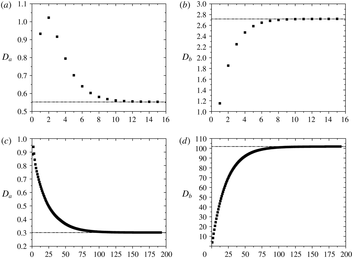
appendix B). We provide a
detailed example on how to conduct the calculation for the first four
reflections in appendix C.
3 Results and discussion
3.1 Approximate formula for drag force
Since the drag force given by (2.58) only includes coefficient
 $B_{2}$
, we approximate the stream function outside the porous
particle (2.19) as
 $$\begin{eqnarray}\unicode[STIX]{x1D6F7}^{e}=\displaystyle rB_{2}C_{2}(\cos \unicode[STIX]{x1D703}).\end{eqnarray}$$
By substituting (3.1) into
(2.56) and using (2.14), the first reflection of
drag force acting on particle
 $A$
(i.e. the first term in (2.54)) can be obtained:
 $$\begin{eqnarray}\boldsymbol{F}_{a}^{(1)}=6\unicode[STIX]{x03C0}\unicode[STIX]{x1D707}a(D_{a}^{(1)}U_{0}+K_{a}^{(1)}U_{a})\boldsymbol{Z},\end{eqnarray}$$
where
 $$\begin{eqnarray}\displaystyle & \displaystyle D_{a}^{(1)}=\displaystyle \frac{2a^{2}[a\unicode[STIX]{x1D6FC}(3R_{0}^{2}\unicode[STIX]{x1D6FC}^{2}-2a^{2}\unicode[STIX]{x1D6FC}^{2}-12)\cosh a\unicode[STIX]{x1D6FC}+(6a^{2}\unicode[STIX]{x1D6FC}^{2}+12-3R_{0}^{2}\unicode[STIX]{x1D6FC}^{2})\sinh a\unicode[STIX]{x1D6FC}]}{3R_{0}^{2}[a\unicode[STIX]{x1D6FC}(3+2a^{2}\unicode[STIX]{x1D6FC}^{2})\cosh a\unicode[STIX]{x1D6FC}-3\sinh a\unicode[STIX]{x1D6FC}]},\qquad & \displaystyle\end{eqnarray}$$
 $$\begin{eqnarray}\displaystyle & \displaystyle K_{a}^{(1)}=\displaystyle \frac{2a^{2}\unicode[STIX]{x1D6FC}^{2}(\sinh a\unicode[STIX]{x1D6FC}-a\unicode[STIX]{x1D6FC}\cosh a\unicode[STIX]{x1D6FC})}{a\unicode[STIX]{x1D6FC}(3+2a^{2}\unicode[STIX]{x1D6FC}^{2})\cosh a\unicode[STIX]{x1D6FC}-3\sinh a\unicode[STIX]{x1D6FC}}.\qquad & \displaystyle\end{eqnarray}$$
Here,
 $K_{ab}^{(1)}$
is zero, since (2.14) has not included the boundary condition of particle
 $B$
. Similarly, by using (2.15), the first reflection of drag force on particle
 $B$
(i.e. the first term in (2.55)) is given by
 $$\begin{eqnarray}\boldsymbol{F}_{b}^{(2)}=6\unicode[STIX]{x03C0}\unicode[STIX]{x1D707}a(D_{b}^{(2)}U_{0}+K_{ba}^{(2)}U_{a}+K_{b}^{(2)}U_{b})\boldsymbol{Z},\end{eqnarray}$$
where
 $$\begin{eqnarray}\displaystyle & & \displaystyle \!\!\!\!\!\displaystyle D_{b}^{(2)}=\nonumber\\ \displaystyle & & \displaystyle \!\!\!\!\!\quad \displaystyle \frac{\displaystyle \left\{\begin{array}{@{}l@{}}\displaystyle \left[\begin{array}{@{}l@{}}3a^{4}b^{4}\unicode[STIX]{x1D6FC}^{4}(6+b^{2}\unicode[STIX]{x1D6FC}^{2}-3L^{2}\unicode[STIX]{x1D6FC}^{2})\\ (12+8a^{2}\unicode[STIX]{x1D6FC}^{2}-3R_{0}^{2}\unicode[STIX]{x1D6FC}^{2}+2a^{4}\unicode[STIX]{x1D6FC}^{4}-a^{2}R_{0}^{2}\unicode[STIX]{x1D6FC}^{4})\\ \quad +\,3ab^{4}L^{3}\unicode[STIX]{x1D6FC}^{4}(3+2a^{2}\unicode[STIX]{x1D6FC}^{2})(12+2b^{2}\unicode[STIX]{x1D6FC}^{2}-3R_{0}^{2}\unicode[STIX]{x1D6FC}^{2})\end{array}\right]\!\cosh a\unicode[STIX]{x1D6FC}\cosh b\unicode[STIX]{x1D6FC}\sinh a\unicode[STIX]{x1D6FC}\\ \quad +\,\displaystyle \left[\begin{array}{@{}l@{}}-4.5a^{3}b^{4}\unicode[STIX]{x1D6FC}^{3}(6+b^{2}\unicode[STIX]{x1D6FC}^{2}-3L^{2}\unicode[STIX]{x1D6FC}^{2})(4+2a^{2}\unicode[STIX]{x1D6FC}^{2}-R_{0}^{2}\unicode[STIX]{x1D6FC}^{2})\\ \quad +\,L^{3}(-9b^{6}\unicode[STIX]{x1D6FC}^{5}-54b^{4}\unicode[STIX]{x1D6FC}^{3}+13.5b^{4}R_{0}^{2}\unicode[STIX]{x1D6FC}^{5})\end{array}\right]\!\cosh b\unicode[STIX]{x1D6FC}\sinh ^{2}a\unicode[STIX]{x1D6FC}\\ \quad +\,\displaystyle \left[\begin{array}{@{}l@{}}13.5a^{3}b^{3}\unicode[STIX]{x1D6FC}^{2}(2+b^{2}\unicode[STIX]{x1D6FC}^{2}-L^{2}\unicode[STIX]{x1D6FC}^{2})(4+2a^{2}\unicode[STIX]{x1D6FC}^{2}-R_{0}^{2}\unicode[STIX]{x1D6FC}^{2})\\ \quad +\,L^{3}(27b^{5}\unicode[STIX]{x1D6FC}^{4}+54b^{3}\unicode[STIX]{x1D6FC}^{2}-13.5b^{3}R_{0}^{2}\unicode[STIX]{x1D6FC}^{4})\end{array}\right]\!\sinh b\unicode[STIX]{x1D6FC}\sinh ^{2}a\unicode[STIX]{x1D6FC}\\ \quad -\,\displaystyle \left[\begin{array}{@{}l@{}}4.5a^{4}b^{3}\unicode[STIX]{x1D6FC}^{3}(2+b^{2}\unicode[STIX]{x1D6FC}^{2}-L^{2}\unicode[STIX]{x1D6FC}^{2})\\ (12-3R_{0}^{2}\unicode[STIX]{x1D6FC}^{2}+2a^{4}\unicode[STIX]{x1D6FC}^{4}+8a^{2}\unicode[STIX]{x1D6FC}^{2}-a^{2}R_{0}^{2}\unicode[STIX]{x1D6FC}^{4})\\ \quad +\,4.5ab^{3}L^{3}\unicode[STIX]{x1D6FC}^{3}(3+2a^{2}\unicode[STIX]{x1D6FC}^{2})(4+2b^{2}\unicode[STIX]{x1D6FC}^{2}-R_{0}^{2}\unicode[STIX]{x1D6FC}^{2})\end{array}\right]\!\sinh b\unicode[STIX]{x1D6FC}\sinh 2a\unicode[STIX]{x1D6FC}\\ \quad -\,\displaystyle \left[\begin{array}{@{}l@{}}0.5a^{5}b^{4}\unicode[STIX]{x1D6FC}^{5}(3+2a^{2}\unicode[STIX]{x1D6FC}^{2})(6+b^{2}\unicode[STIX]{x1D6FC}^{2}-3L^{2}\unicode[STIX]{x1D6FC}^{2})\\ (12+2a^{2}\unicode[STIX]{x1D6FC}^{2}-3R_{0}^{2}\unicode[STIX]{x1D6FC}^{2})\\ \quad +\,0.5a^{2}b^{4}L^{3}\unicode[STIX]{x1D6FC}^{5}(3+2a^{2}\unicode[STIX]{x1D6FC}^{2})^{2}(12+2b^{2}\unicode[STIX]{x1D6FC}^{2}-3R_{0}^{2}\unicode[STIX]{x1D6FC}^{2})\end{array}\right]\!\cosh b\unicode[STIX]{x1D6FC}\cosh ^{2}a\unicode[STIX]{x1D6FC}\\ \quad +\,\displaystyle \left[\begin{array}{@{}l@{}}1.5a^{5}b^{3}\unicode[STIX]{x1D6FC}^{4}(3+2a^{2}\unicode[STIX]{x1D6FC}^{2})(2+b^{2}\unicode[STIX]{x1D6FC}^{2}-L^{2}\unicode[STIX]{x1D6FC}^{2})\\ (12+2a^{2}\unicode[STIX]{x1D6FC}^{2}-3R_{0}^{2}\unicode[STIX]{x1D6FC}^{2})\\ \quad +\,1.5a^{2}b^{3}L^{3}\unicode[STIX]{x1D6FC}^{4}(3+2a^{2}\unicode[STIX]{x1D6FC}^{2})^{2}(4+2b^{2}\unicode[STIX]{x1D6FC}^{2}-R_{0}^{2}\unicode[STIX]{x1D6FC}^{2})\end{array}\right]\!\sinh b\unicode[STIX]{x1D6FC}\cosh ^{2}a\unicode[STIX]{x1D6FC}\end{array}\right\}}{\displaystyle 3a\unicode[STIX]{x1D6FC}^{2}L^{3}R_{0}^{2}[(3b\unicode[STIX]{x1D6FC}+2b^{3}\unicode[STIX]{x1D6FC}^{3})\cosh b\unicode[STIX]{x1D6FC}-3\sinh b\unicode[STIX]{x1D6FC}][(1.5a\unicode[STIX]{x1D6FC}+a^{3}\unicode[STIX]{x1D6FC}^{3})\cosh a\unicode[STIX]{x1D6FC}-1.5\sinh a\unicode[STIX]{x1D6FC}]^{2}},\nonumber\\ \displaystyle & & \displaystyle\end{eqnarray}$$
 $$\begin{eqnarray}\displaystyle & & \displaystyle \!\!\!\!\!K_{ba}^{(2)}=\nonumber\\ \displaystyle & & \displaystyle \!\!\!\!\!\quad \displaystyle \displaystyle \frac{\displaystyle 2a^{3}\unicode[STIX]{x1D6FC}^{2}b^{3}\displaystyle \!\left(\begin{array}{@{}l@{}}3a^{2}\unicode[STIX]{x1D6FC}^{2}\cosh ^{2}a\unicode[STIX]{x1D6FC}+2a^{4}\unicode[STIX]{x1D6FC}^{4}\cosh ^{2}a\unicode[STIX]{x1D6FC}\\ \quad +\,3\sinh ^{2}a\unicode[STIX]{x1D6FC}-3a\unicode[STIX]{x1D6FC}\sinh 2a\unicode[STIX]{x1D6FC}\\ \quad -\,a^{3}\unicode[STIX]{x1D6FC}^{3}\sinh 2a\unicode[STIX]{x1D6FC}\end{array}\right)\!\displaystyle \left(\begin{array}{@{}l@{}}6b\unicode[STIX]{x1D6FC}\cosh b\unicode[STIX]{x1D6FC}-5b^{3}\unicode[STIX]{x1D6FC}^{3}\cosh b\unicode[STIX]{x1D6FC}\\ \quad +\,15bL^{2}\unicode[STIX]{x1D6FC}^{3}\cosh b\unicode[STIX]{x1D6FC}-6\sinh b\unicode[STIX]{x1D6FC}\\ \quad +\,3b^{2}\unicode[STIX]{x1D6FC}^{2}\sinh b\unicode[STIX]{x1D6FC}-15L^{2}\unicode[STIX]{x1D6FC}^{2}\sinh b\unicode[STIX]{x1D6FC}\end{array}\right)}{\displaystyle 5aL^{3}[(3a\unicode[STIX]{x1D6FC}+2a^{3}\unicode[STIX]{x1D6FC}^{3})\cosh a\unicode[STIX]{x1D6FC}-3\sinh a\unicode[STIX]{x1D6FC}]^{2}[b\unicode[STIX]{x1D6FC}(3+2b^{2}\unicode[STIX]{x1D6FC}^{2})\cosh b\unicode[STIX]{x1D6FC}-3\sinh b\unicode[STIX]{x1D6FC}]},\nonumber\\ \displaystyle & & \displaystyle\end{eqnarray}$$
 $$\begin{eqnarray}\displaystyle & \displaystyle K_{b}^{(2)}=\displaystyle \frac{2b^{3}\unicode[STIX]{x1D6FC}^{2}(\sinh b\unicode[STIX]{x1D6FC}-b\unicode[STIX]{x1D6FC}\cosh b\unicode[STIX]{x1D6FC})}{(3ab\unicode[STIX]{x1D6FC}+2ab^{3}\unicode[STIX]{x1D6FC}^{3})\cosh b\unicode[STIX]{x1D6FC}-3a\sinh b\unicode[STIX]{x1D6FC}}. & \displaystyle\end{eqnarray}$$
Thus far, we have derived the first term of (2.55), given by (3.5), as the approximate drag force to the first
leading order acting on particle
 $B$
, in which the boundary conditions of particle
 $A$
, particle
 $B$
and the cylindrical tube have been taken into account.
Following the same procedure as above, the approximate drag acting on particle
 $A$
is simply (3.5) by exchanging the letters
 $b$
and
 $a$
.
3.2 Model validation
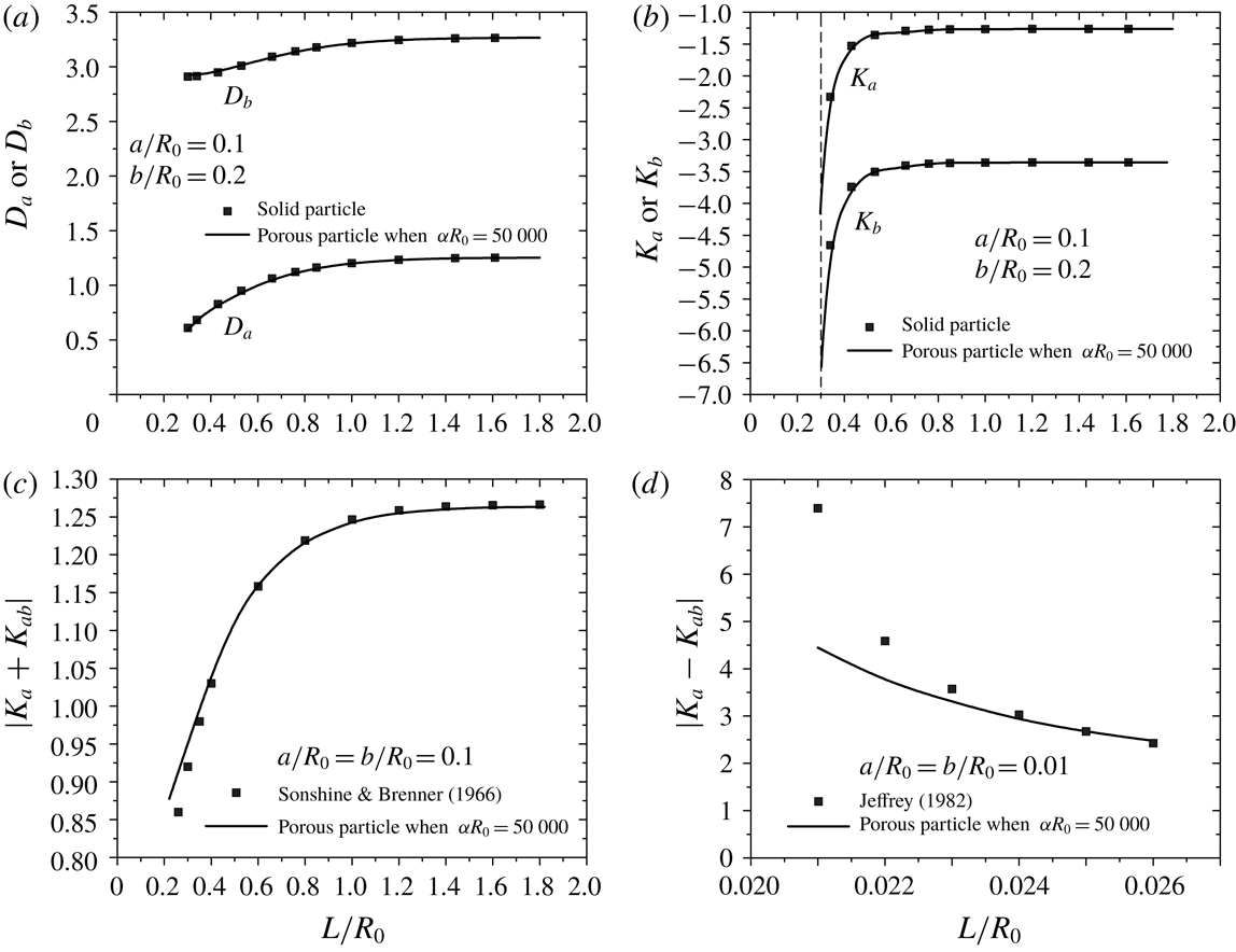
Drag force coefficients (a)
 $D_{a}$
or
 $D_{b}$
and (b)
 $K_{a}$
or
 $K_{b}$
when
 $a/R_{0}=0.1$
,
 $b/R_{0}=0.2$
. (c)
 $|K_{a}+K_{ab}|$
when
 $a/R_{0}=b/R_{0}=0.1$
. (d)
 $|K_{a}-K_{ab}|$
when
 $a/R_{0}=b/R_{0}=0.01$
. All the drag force coefficients are plotted as a
function of the normalized distance
 $L/R_{0}$
.

In this section, we validate our semi-analytical solution with previous
works, where the motion of two solid particles has been studied. As
 $\unicode[STIX]{x1D6FC}$
goes to infinity, the permeability approaches zero and the
particle becomes a solid sphere. We first validate our full model solution
with our previous work (Yao et al.
Reference Yao and Wong2017), which is also based on the
method of reflections. We consider the case
 $a/R_{0}=0.1$
,
 $b/R_{0}=0.2$
and
 $\unicode[STIX]{x1D6FC}R_{0}=50\,000$
by using the procedures introduced in § 2. At such a large
 $\unicode[STIX]{x1D6FC}$
, the fluid going through the internal region is extremely
limited and can be approximated as the solid particle case. Figure 2(a,b)
shows that the drag force coefficients due to the background flow (
 $D_{a}$
and
 $D_{b}$
) and particle velocities (
 $K_{a}$
and
 $K_{b}$
) evaluated at
 $\unicode[STIX]{x1D6FC}R_{0}=50\,000$
are in good agreement with our previous work (Yao
et al.
Reference Yao and Wong2017). This has confirmed the
consistency of the two frameworks. Moreover, Sonshine & Brenner
(Reference Sonshine and Brenner1966) theoretically investigated
the motion of two or more solid particles travelling along the axis of a
cylindrical tube without the background flow by developing the point force
formula based on the stream function. The particles are equally spaced along
the axis and translate with a constant velocity. We compare our solution
with their work for the case that (
 $a/R_{0}=b/R_{0}=0.1$
,
 $\unicode[STIX]{x1D6FC}R_{0}=50\,000$
) (figure 2
c). We can clearly see that the drag force coefficients
calculated from our full semi-analytical results are in good agreement with
the previous work except when the two particles are very close (
 $L/R_{0}<0.3$
). In addition, the drag force of two identical particles
approaching each other with a constant velocity in an unbounded fluid based
on the lubrication theory has been previously solved (Jeffrey Reference Jeffrey1982). We then consider the case
 $a/R_{0}=b/R_{0}=0.01$
and
 $\unicode[STIX]{x1D6FC}R_{0}=50\,000$
by using the procedures introduced in § 2 to compare with the lubrication theory
solution. In such a case of a small particle size, the wall effect in our
solution is negligible. It should be noted that when the two particles are
very close, our solution cannot match with the lubrication theory solution
(figure 2
d). This could be due to the fact that the method of
reflections is not accurate to solve cases when the two solid particles (
 $\unicode[STIX]{x1D6FC}R_{0}=50\,000$
) are very close, consistent with what is reported in the
literature (Bhattacharya et al.
Reference Bhattacharya, Mishra and Bhattacharya2010).
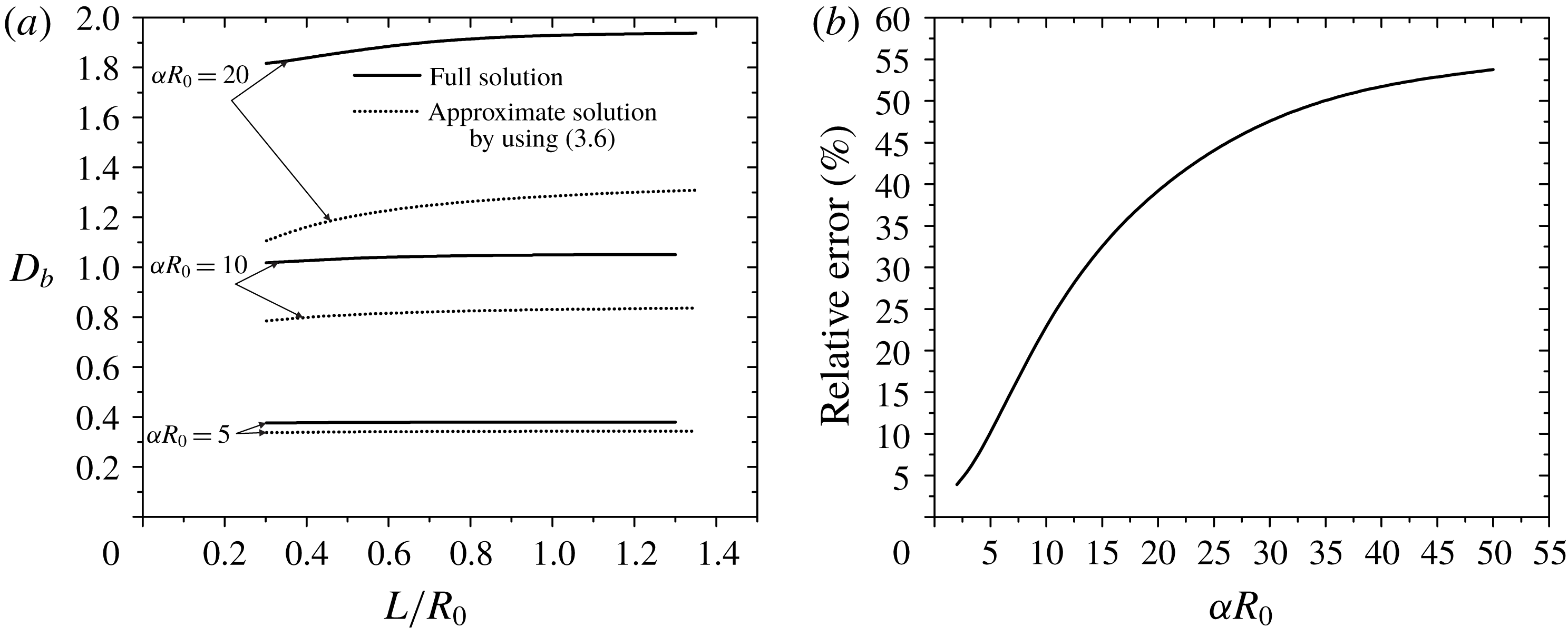
(a) Drag force coefficient
 $D_{b}$
as a function of normalized distance
 $L/R_{0}$
for
 $\unicode[STIX]{x1D6FC}R_{0}=5,10,20$
. (b) Relative error as a
function of
 $\unicode[STIX]{x1D6FC}R_{0}$
.

Here, we present the validation of the approximate solution derived
in § 3.1. In figure 3(a), we compare our full
semi-analytical results with the approximate solution given by (3.6) when
 $a/R_{0}=0.1$
,
 $b/R_{0}=0.2$
and
 $\unicode[STIX]{x1D6FC}R_{0}=5,10,20$
. As
 $\unicode[STIX]{x1D6FC}R_{0}$
increases,
 $D_{b}$
increases, which indicates the porous particle experiences
a larger drag force due to the background flow. Since (3.6) is the approximate
expression of the drag force, it is not unexpected that the magnitude is
smaller than that of the full semi-analytical solution. As
 $\unicode[STIX]{x1D6FC}R_{0}$
decreases, the difference between (3.6) and the semi-analytical
result becomes smaller (figure 3
a), which implies that the particles’ contribution to the
drag force is not as important. To better highlight this, we investigate the
effect of
 $\unicode[STIX]{x1D6FC}R_{0}$
on the relative error between the full semi-analytical
solution and the approximate solution for
 $a/R_{0}=0.1$
,
 $b/R_{0}=0.2$
and
 $L/R_{0}=0.301$
. Figure 3(b) demonstrates that the decrease in
 $\unicode[STIX]{x1D6FC}R_{0}$
leads to the decrease in the relative error. When
 $\unicode[STIX]{x1D6FC}R_{0}$
is smaller than 5, the relative error is less than 10 %
which indicates that (3.6)
is a good approximate solution of the drag force acting on the porous
particle. We repeated our calculations for (3.7)–(3.8) and found again that these approximate solutions are valid when
 $\unicode[STIX]{x1D6FC}R_{0}$
is smaller than 5. We can also infer that the
particle–particle interaction decreases as
 $\unicode[STIX]{x1D6FC}R_{0}$
decreases.
3.3 Two identical particles moving along the axis of the tube
Previous works have investigated the permeability of porous media
theoretically and experimentally. Kapur et al. (Reference Kapur, Charkoudian, Kessler and Anderson1996) measured the permeability of
polymer gels when they are stabilized within a microporous support. Mika
& Childs (Reference Mika and Childs2001) developed a
model in which gel networks are considered as an assemblage of spheres to
calculate the hydrodynamic permeability. They have provided the equation to
calculated the radius
 $a_{p}$
of such spheres. Theoretical works have provided the
equations to calculate the hydrodynamic permeability based on
 $a_{p}$
and porosity
 $\unicode[STIX]{x1D700}$
. One of the most widely used equations to calculate the
permeability is from Brinkman (Reference Brinkman1949):
 $$\begin{eqnarray}k=\displaystyle \frac{a_{p}^{2}}{18}\left(3+\frac{4}{1-\unicode[STIX]{x1D700}}-3\sqrt{\frac{8}{1-\unicode[STIX]{x1D700}}-3}\right).\end{eqnarray}$$
Happel & Brenner (Reference Happel and Brenner1983) have also derived the relationship based on the cell model method (Mika & Childs Reference Mika and Childs2001):
 $$\begin{eqnarray}k=\displaystyle \frac{2a_{p}^{2}}{9(1-\unicode[STIX]{x1D700})}\left[\frac{3-4.5(1-\unicode[STIX]{x1D700})^{1/3}+4.5(1-\unicode[STIX]{x1D700})^{5/3}-3(1-\unicode[STIX]{x1D700})^{2}}{3+2(1-\unicode[STIX]{x1D700})^{5/3}}\right].\end{eqnarray}$$
Mika & Childs (Reference Mika and Childs2001) have shown the comparison between the theoretical work and experimental data conducted by Kapur et al. (Reference Kapur, Charkoudian, Kessler and Anderson1996) and both equations (3.9)–(3.10) give a good prediction of the permeability of the gel. In addition, the permeability can be predicted with the Carman–Kozeny formula (Krainov, Smirnov & Tereshonok Reference Krainov, Smirnov and Tereshonok2014):
 $$\begin{eqnarray}k=\displaystyle \frac{\unicode[STIX]{x1D700}^{3}a_{p}^{2}}{45(1-\unicode[STIX]{x1D700})^{2}}.\end{eqnarray}$$
In our study, we consider a material with a large porosity, such as a
polymer gel with porosity
 $\unicode[STIX]{x1D700}=0.96$
. Based on the equation and parameters from Mika &
Childs (Reference Mika and Childs2001), we can calculate
 $a_{p}=2.66\times 10^{-10}/\sqrt{0.372(1-\unicode[STIX]{x1D700})}$
m. Using (3.9)–(3.11),
 $\unicode[STIX]{x1D6FC}=\sqrt{1/k}$
can be obtained. In our main discussion, we choose
 $\unicode[STIX]{x1D6FC}R_{0}=40$
and
 $\unicode[STIX]{x1D6FC}R_{0}=100$
. Using these values, we summarized the calculated values of
 $a_{p}$
,
 $\unicode[STIX]{x1D6FC}$
and
 $R_{0}$
in tables 1
and 2. The experiments of Kapur
et al. (Reference Kapur, Charkoudian, Kessler and Anderson1996)
reported a value of
 $\unicode[STIX]{x1D6FC}=2.26\times 10^{8}~\text{m}^{-1}$
. Using this value, we also calculated the corresponding
 $R_{0}$
in tables 1
and 2.
Variables corresponding to
 $\unicode[STIX]{x1D6FC}R_{0}=\sqrt{1/k}R_{0}=40$
.

Variables corresponding to
 $\unicode[STIX]{x1D6FC}R_{0}=\sqrt{1/k}R_{0}=100$
.

It can be seen that
 $R_{0}$
is at least one order larger than
 $a_{p}$
. In our study, the minimum size of the porous particle is
 $a/R_{0}=0.1$
and
 $a$
is at least six times larger than
 $a_{p}$
. Although the Brinkman equation is only fully accurate for
 $a_{p}/a\ll 1$
, it can be used as a first-order approximation in
 $a_{p}/a$
provided that
 $a_{p}/a<1$
(Auriault Reference Auriault2009). It
should be noted that
 $R_{0}$
is in the nanometer scale based on our calculation result.
This nanoscale of fluidic structures is of interest for a great variety of
applications, ranging from drug delivery (Sinha et al.
Reference Sinha, Valco, Sharma, Liu and Ferrari2004) and energy transfer (Daiguji
et al.
Reference Daiguji, Yang, Szeri and Majumdar2004; van der Heyden et al.
Reference van der Heyden, Bonthuis, Stein, Meyer and Dekker2006) to biochemical analysis (Foquet
et al.
Reference Foquet, Korlach, Zipfel, Webb and Craighead2002). Previous works have shown the
procedure to fabricate the nanochannel. Lee et al. (Reference Lee, Yang, Myung and George2003) have developed a nanochannel
fabrication technique by using chemical–mechanical polishing and thermal
oxidation. They have successfully fabricated narrow channels (i.e. 10 mm
long, 25 nm wide and 100 nm deep) with smooth inner surfaces. Song
et al. (Reference Song, Kim, Kwon, Kim and Kim2012)
have fabricated nanochannels by utilizing the crystallinity-dependent
anisotropic wet etching of silicon. The dimension of the nanochannel is down
to 16 nm in depth and 175 nm in width and up to 8 cm in length. Even at such
a scale, the Stokes equation and Brinkman equation are still valid (Urbakh,
Daikhin & Klafter Reference Urbakh, Daikhin and Klafter1995;
Bocquet & Charlaix Reference Bocquet and Charlaix2010).
We first consider two identical porous particles moving along the axis of
the tube (
 $a/R_{0}=b/R_{0}=0.1$
and
 $a/R_{0}=b/R_{0}=0.3$
) with
 $\unicode[STIX]{x1D6FC}R_{0}=40$
and
 $\unicode[STIX]{x1D6FC}R_{0}=100$
. The semi-analytical results such as drag force
coefficients and particle velocities are plotted against the normalized
separation distance between the two particles
 $L/R_{0}$
. Due to kinematic reversibility at low Reynolds number,
the coefficients of the two identical particles are expected to be
identical. Our semi-analytical results have also verified that this is the
case. For convenience, the new variables
 $D(D=D_{a}=D_{b}),K(K=K_{a}=K_{b})$
and
 $K^{\ast }(K^{\ast }=K_{ab}=K_{ba})$
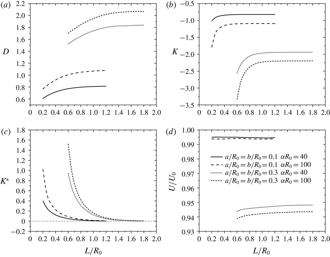
are utilized to represent the coefficients (figure 4
a–c).
Drag force coefficients and normalized velocity of two identical
porous particles. (a) Drag force coefficient
 $D$
; (b) drag force coefficient
 $K$
; (c) drag force coefficient
 $K^{\ast }$
and (d) normalized particle
velocities
 $U=U_{a}=U_{b}$
. Two particle sizes and two
 $\unicode[STIX]{x1D6FC}R_{0}$
are considered:
 $a/R_{0}=b/R_{0}=0.1,0.3$
;
 $\unicode[STIX]{x1D6FC}R_{0}=40,100$
.

The coefficient
 $D$
(figure 4
a), describing the drag force due to the background flow on
the particles when they are at rest, increases monotonically from a minimum
to a constant value. At small separation distance
 $L/R_{0}$
, the effect of particle interaction is strong inducing a
small velocity gradient between them and thus a small drag force. Details of
the streamlines and velocity contour will be discussed below. As
 $L/R_{0}$
increases, the effect of particle interaction diminishes
and each particle behaves as a single particle case, indicated by the constant
 $D$
. In addition, bigger particles have larger drag force
coefficients due to the stronger wall effect. When
 $\unicode[STIX]{x1D6FC}R_{0}$
is larger (
 $\unicode[STIX]{x1D6FC}R_{0}=100$
), the particle has a smaller permeability, hence it is
harder for the fluid to go through the internal region of the particle. The
porous particle experiences a larger drag force than that with a smaller
 $\unicode[STIX]{x1D6FC}R_{0}$
(
 $\unicode[STIX]{x1D6FC}R_{0}=40$
). Thus, as
 $\unicode[STIX]{x1D6FC}R_{0}$
increases, the coefficient
 $D$
has a similar relationship with
 $L/R_{0}$
, but with a larger magnitude.
Unlike the coefficient
 $D$
,
 $K$
represents the drag force contribution due to the movement
of one particle while the other is at rest in the absence of the background
flow (figure 4
b). This drag force is against the direction of the
particle motion, which explains the negative sign of
 $K$
. When the particle is moving in the fluid, the presence of
the neighbouring resting particle increases the velocity gradient in the
vicinity of the moving particle and thus also increases the drag force
acting on the moving particle. This effect is more pronounced as the two
particles get closer due to stronger particle–particle interaction. As the
separation distance
 $L/R_{0}$
increases,
 $K$
approaches the single particle case. In addition, smaller
 $\unicode[STIX]{x1D6FC}R_{0}$
allows the fluid to smoothly pass through the particle,
represented by the smaller coefficient
 $K$
magnitude. Unsurprisingly, we also found that bigger
particles have a larger drag force magnitude due to the stronger wall
effect.
The drag coefficient
 $K^{\ast }$
represents the particle–particle interaction in the
absence of background flow (figure 4
c). It describes the drag force acting on a resting
particle due to the movement of the neighbouring particle. The coefficient
 $K^{\ast }$
is positive since the drag force is in the same direction
as the moving particle. When the neighbouring particle is moving, it drags
the surrounding fluid inducing drag force on the resting particle. As the
two particles get very close, the coefficient
 $K^{\ast }$
reaches its maximum value, which arises from a large shear
rate in the gap between the two particles. It is not unexpected that as
 $L/R_{0}$
increases,
 $K^{\ast }$
decays to zero since the hydrodynamic interaction becomes
negligible.
As mentioned earlier, the velocities of particles can be calculated by
applying zero total drag force due to the negligible inertia effect at low
Reynolds number. The velocity of particle
 $A$
is the same as particle
 $B$
since the two particles are identical (
 $U=U_{a}=U_{b}$
), which implies the two particles will not attract nor
repel. This is consistent with the kinematic reversibility argument.
Figure 4(d) shows
that the particle velocity is almost unaffected by the separation distance
 $L/R_{0}$
, with the smallest magnitude when the two particles are
almost in contact. We also find that smaller
 $\unicode[STIX]{x1D6FC}R_{0}$
gives rise to larger particle velocity, as it is easier
for the fluid to go through the particle. When the particle is bigger, it
possesses a smaller velocity due to the non-uniformity of the background
parabolic flow as well as the interaction with the cylinder wall.
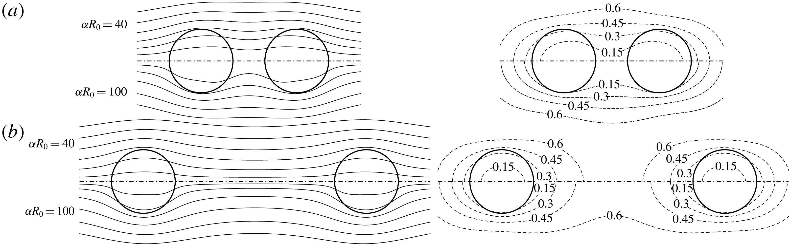
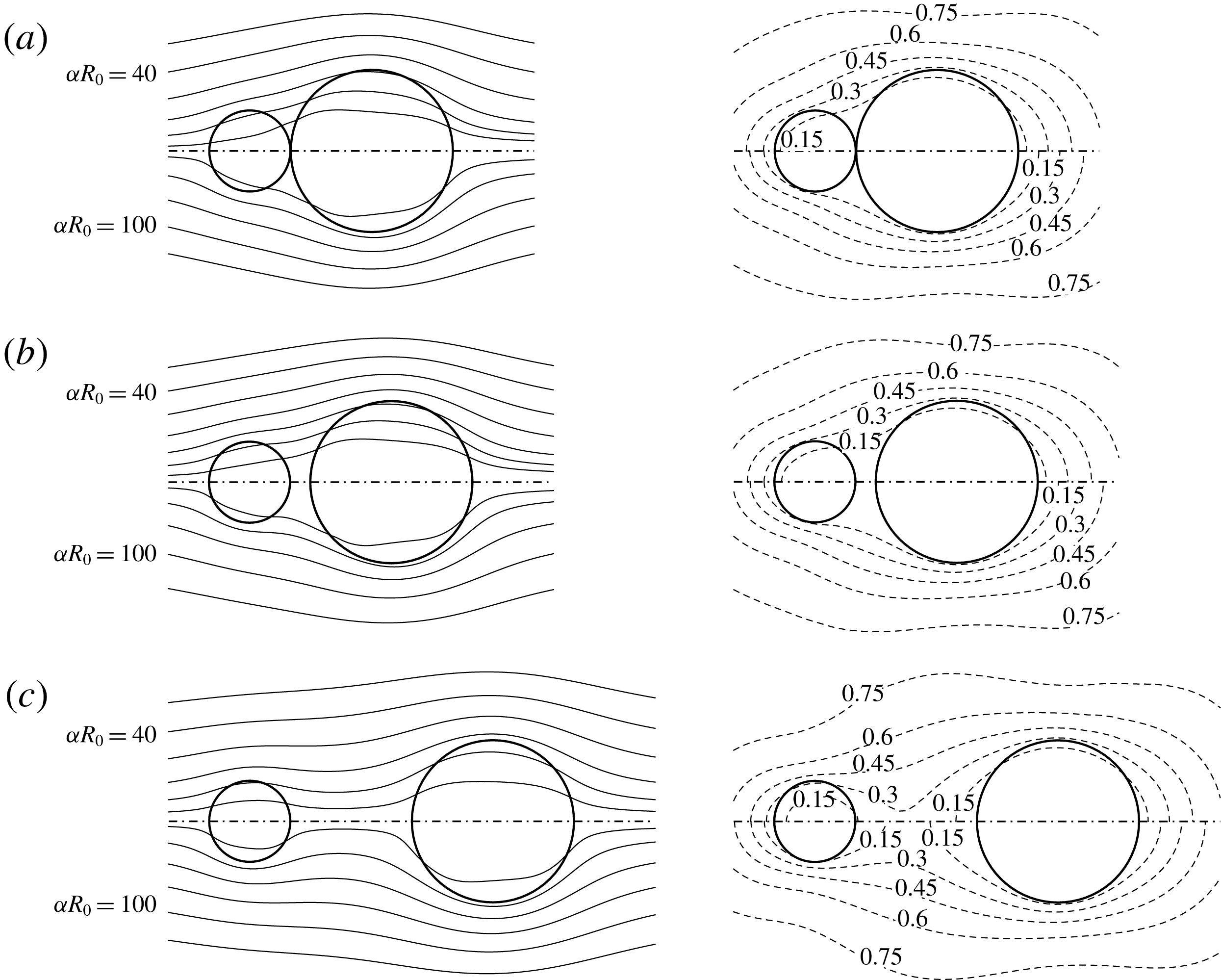
To better highlight the hydrodynamic interaction between the two porous
particles, we choose two representative separation distances (
 $L/R_{0}=0.3,0.7$
) with
 $a/R_{0}=b/R_{0}=0.1$
and
 $\unicode[STIX]{x1D6FC}R_{0}=40,100$
, to investigate the corresponding streamlines and velocity
contour in the
 $Z$
-direction in the vicinity of the two particles
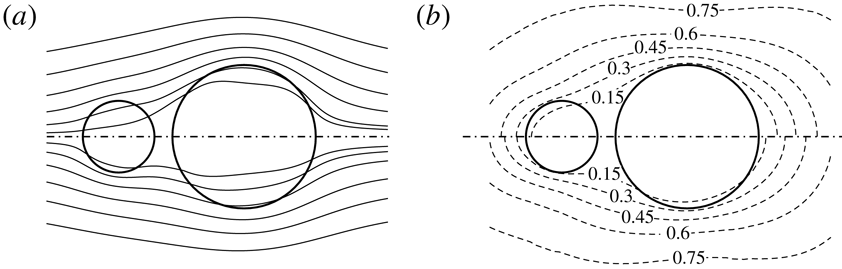
(figure 5) when they are fixed. The
pattern of the streamlines is related to the permeability of the particle.
Large permeability (small
 $\unicode[STIX]{x1D6FC}R_{0}$
) allows fluid to go through the internal region of the
particle easily, and thus results in streamlines that are almost parallel to
the axis of the tube (top half of figure 5
a,b). Due to higher fluid resistance to
move through the porous particle, the
 $Z$
-direction velocity of the fluid inside the particle is
smaller than that outside. When
 $\unicode[STIX]{x1D6FC}R_{0}=100$
, the particle is less permeable, inducing evident
distortion of the streamlines in the vicinity of the two particles (bottom
half of figure 5
a,b). The streamlines and velocity contour
are squeezed towards the wall of the tube. The
 $Z$
-direction velocity of the fluid in the vicinity of the two
particles is smaller than that of
 $\unicode[STIX]{x1D6FC}R_{0}=40$
because of the higher fluid resistance inside the
particle. The velocity contour is denser when
 $\unicode[STIX]{x1D6FC}R_{0}$
is larger indicating larger shear rates, which explains
why the particle with larger
 $\unicode[STIX]{x1D6FC}R_{0}$
experiences a larger drag force than that with smaller
 $\unicode[STIX]{x1D6FC}R_{0}$
. The effect of separation distance
 $L/R_{0}$
on the velocity field can also be seen from figure 5. At small
 $L/R_{0}$
, the boundary layers of the two particles interact and
thus as the streamline exits the first particle, it does not recover to its
upstream condition before entering the second particle (figure 5
a). Such distortion is not visible when the two particles
are far apart (figure 5
b). The fluid in the gap between the two particles
experiences smaller shear rate when they are close to each other.
Streamlines (left) and normalized velocity contour in the
 $Z$
-direction
 $v_{Z}/U_{0}$
(right) around two identical particles
 $a/R_{0}=b/R_{0}=0.1$
. Since it is an axisymmetric model, we only plot
half of the region of the flow field:
 $\unicode[STIX]{x1D6FC}R_{0}=40$
(top half) and
 $\unicode[STIX]{x1D6FC}R_{0}=100$
(bottom half). Two representative separation
distances are considered:
 $L/R_{0}=0.3$
(a) and
 $L/R_{0}=0.7$
(b).

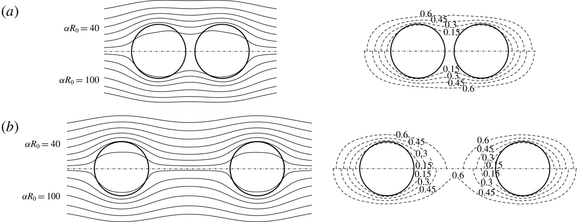
Figure 6 shows the streamlines and
velocity contour in the
 $Z$
-direction around two identical particles when
 $a/R_{0}=b/R_{0}=0.3$
. We can see that the distortion of the streamlines is more
significant since the two particles are bigger than those presented in
figure 5. The velocity contour
further reinforces this phenomenon. Here, the particles squeeze the
streamlines towards the wall and the velocity contours in the vicinity
around the boundary of the particle are denser than that in figure 5. As mentioned earlier, the denser
velocity contour indicates a larger velocity gradient, which results in a
larger drag force. The effect of
 $\unicode[STIX]{x1D6FC}R_{0}$
on the velocity field for the larger particles here is
similar to that in figure 5. However,
it is interesting to note that even though the background velocity is
parabolic and the local fluid velocity moving at the axis of the tube is
maximum, we find that the velocity of the fluid inside the particle is
smaller than the velocity of the fluid outside the particle nearer to the
wall, due to the fluid resistance inside the particle. This effect is more
evident when the particle is bigger with sufficiently large
 $\unicode[STIX]{x1D6FC}R_{0}$
(i.e. sufficiently large fluid resistance). In the limit
of
 $\unicode[STIX]{x1D6FC}R_{0}$
approaching zero, the particle is completely permeable
(simply becomes a control volume), the velocity field will therefore be
unaffected regardless of the size of the particle.
Streamlines (left) and normalized velocity contour in the
 $Z$
-direction
 $v_{z}/U_{0}$
(right) around two identical particles
 $a/R_{0}=b/R_{0}=0.3$
. Since it is an axisymmetric model, we only plot
half of the region of the flow field:
 $\unicode[STIX]{x1D6FC}R_{0}=40$
(top half) and
 $\unicode[STIX]{x1D6FC}R_{0}=100$
(bottom half). Two representative separation
distances are considered:
 $L/R_{0}=0.7$
(a) and
 $L/R_{0}=1.5$
(b).

3.4 Two particles with unequal sizes moving along the axis of the tube
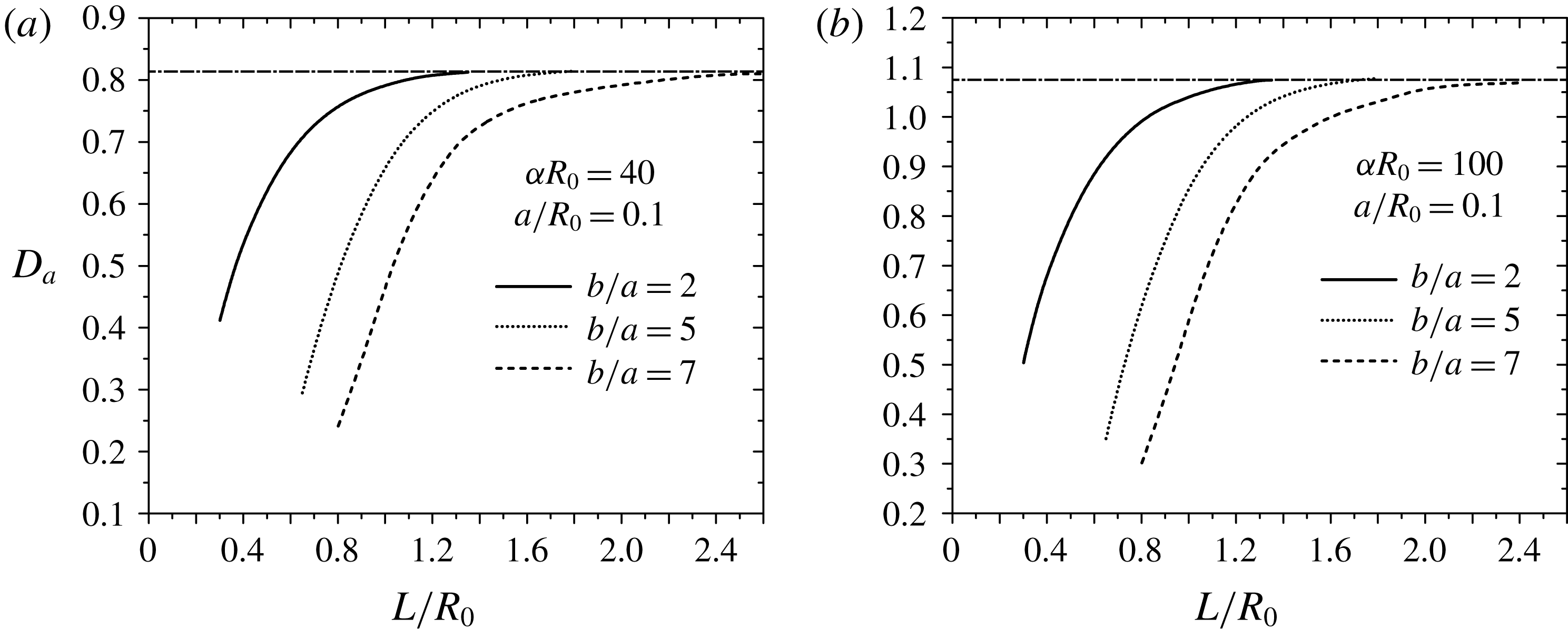
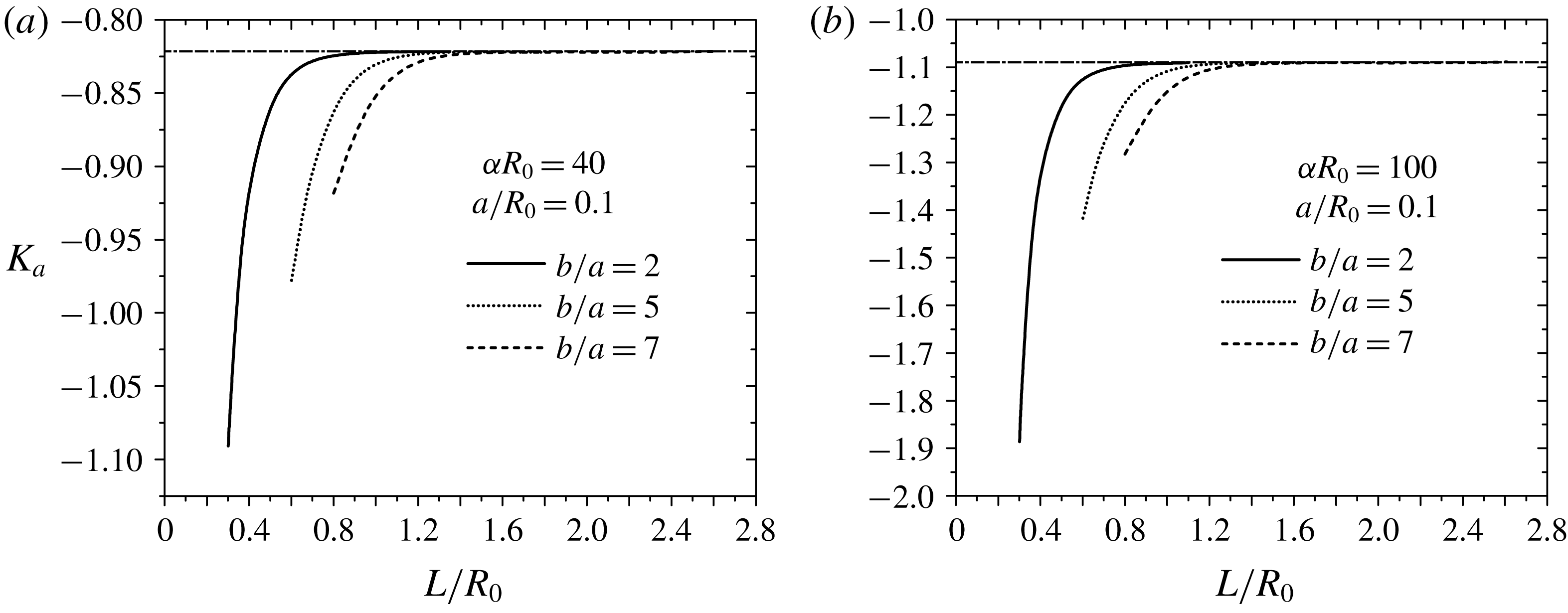
Drag force coefficient
 $D_{a}$
of particle size ratio
 $b/a=2,5,7$
for
 $\unicode[STIX]{x1D6FC}R_{0}=40$
(a) and
 $\unicode[STIX]{x1D6FC}R_{0}=100$
(b). The size of particle
 $A$
,
 $a/R_{0}=0.1$
. The horizontal line refers to the single
particle case.

We now consider the case when the two particles are unequal. We keep the
size of particle
 $A$
as
 $a/R_{0}=0.1$
and vary the radius of particle
 $B$
with
 $b/a=2,5,7$
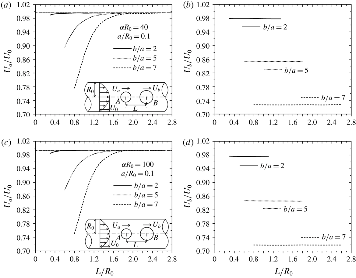
. Figure 7 shows the
normalized drag force coefficient
 $D_{a}$
. As mentioned previously, when the two particles are close
to each other, a larger region where the velocity gradient of the fluid is
small is induced between them that causes the smaller
 $D_{a}$
. As the separation distance
 $L/R_{0}$
increases,
 $D_{a}$
approaches the single particle result. Such an effect is
more pronounced with the bigger sizes of particle
 $B$
(
 $b/a=2,5,7$
) due to the stronger particle–particle interaction.
Similar to figure 4(a), the permeability influences the drag force.
When the particle’s permeability is small (
 $\unicode[STIX]{x1D6FC}R_{0}=100$
, figure 7
b), it is harder for the fluid to go through the internal
region of the particle resulting in a larger drag force on particle
 $A$
. At larger permeability (
 $\unicode[STIX]{x1D6FC}R_{0}=40$
, figure 7
a), the flow field is more parallel and the
particle–particle interaction has relatively less effect on the particle’s
motion, which causes smaller
 $D_{a}$
magnitude as well as smaller variation of
 $D_{a}$
against
 $L/R_{0}$
.
Drag force coefficient
 $D_{b}$
of particle size ratio
 $b/a=2$
(a,b),
 $b/a=5$
(c,d),
 $b/a=7$
(e,f). The size
of particle
 $A$
,
 $a/R_{0}=0.1$
;
 $\unicode[STIX]{x1D6FC}R_{0}=40$
(a,c,e) and
 $\unicode[STIX]{x1D6FC}R_{0}=100$
(b,d,f). The
horizontal line refers to the single particle case.

Streamlines (left) and normalized velocity contour in the
 $Z$
-direction
 $v_{z}/U_{0}$
(right) around two particles
 $a/R_{0}=0.1$
and
 $b/a=2$
. Since it is an axisymmetric model, we only plot
half of the region of the flow field:
 $\unicode[STIX]{x1D6FC}R_{0}=40$
(top half) and
 $\unicode[STIX]{x1D6FC}R_{0}=100$
(bottom half). Three representative separation
distances are considered:
 $L/R_{0}=0.301$
(a),
 $L/R_{0}=0.35$
(b), and
 $L/R_{0}=0.6$
(c). The three representative
 $L/R_{0}$
have been marked in figure 8(a,b).

Figure 8 shows the variation of the
coefficient
 $D_{b}$
against separation distance
 $L/R_{0}$
. Interestingly,
 $D_{b}$
does not vary monotonously when particle
 $B$
is bigger than particle
 $A$
except for
 $a/R_{0}=0.1$
,
 $b/R_{0}=0.2$
and
 $\unicode[STIX]{x1D6FC}R_{0}=40$
(figure 8
a). As
 $L/R_{0}$
increases, the coefficient
 $D_{b}$
decreases first to a minimum value and then increases to a
constant representing the single particle case. Similar to
 $D_{a}$
, smaller permeability (
 $\unicode[STIX]{x1D6FC}R_{0}=100$
) causes the porous particle to experience a larger
 $D_{b}$
(figure 8
b,d,f).
To investigate the detailed flow field around the two particles, we choose
three representative separation distances (
 $L/R_{0}=0.301$
, 0.35 and 0.6) with
 $b/a=2$
when
 $\unicode[STIX]{x1D6FC}R_{0}=40$
and 100 and plot the corresponding streamlines and
velocity contour in the
 $Z$
-direction in the vicinity of the two particles when they
are fixed along the axis (figure 9).
The permeability of the particle and separation distance
 $L/R_{0}$
can significantly affect the flow field. At
 $\unicode[STIX]{x1D6FC}R_{0}=40$
(top half), it is easier for the fluid to pass through the
two particles and the streamlines are almost parallel to the axis of the
tube with smaller distortion. In addition, a bigger particle can induce
larger distortion and the streamlines are squeezed towards the wall when the
fluid passes through particle
 $B$
. As discussed earlier, due to the resistance inside the
porous particle, the fluid has a smaller
 $Z$
-direction velocity inside the particle than that outside.
This phenomenon is more evident for larger particle
 $B$
. At
 $\unicode[STIX]{x1D6FC}R_{0}=100$
(bottom half), the particle has smaller permeability and
the fluid tends to move around the particle. Especially in the vicinity of particle
 $B$
, the streamlines are extremely squeezed and more fluid
flows outside the particle. Furthermore, the velocity contour at
 $\unicode[STIX]{x1D6FC}R_{0}=100$
is stretched outwards as compared with
 $\unicode[STIX]{x1D6FC}R_{0}=40$
due to the larger distortion. Such an effect causes the
velocity contour to become denser around the two particles, which is more
apparent around particle
 $B$
. Since a dense velocity contour indicates a large velocity
gradient, the two particles experience a large drag force, which agrees with
that previously discussed (figures 5
and 6). Taking a closer look at the
velocity contour of
 $\unicode[STIX]{x1D6FC}R_{0}=40$
, when the two particles are almost in contact
(figure 9
a top half) and when the two particles are slightly apart
(figure 9
b top half), the contour looks almost identical, except
that the contour is slightly denser in figure 9(b). When the separation distance
 $L/R_{0}$
is even larger (figure 9
c top half), the velocity contour is even denser. This
explains the monotonic increase in
 $D_{b}$
in figure 8(a). However, for small permeability (
 $\unicode[STIX]{x1D6FC}R_{0}=100$
), the velocity contour when the two particles are almost
in contact is denser than that when the two particles are slightly apart
(figure 9
a,b bottom half). When the separation
distance
 $L/R_{0}$
is large (figure 9
c bottom half), the velocity contour is denser than that in
figure 9(a,b) (bottom half). The
corresponding drag coefficient
 $D_{b}$
is therefore observed to decrease at small
 $L/R_{0}$
and increase at large
 $L/R_{0}$
(figure 8
b).
Drag force coefficient
 $K_{a}$
of various particle size ratios
 $b/a=2,5,7$
with
 $\unicode[STIX]{x1D6FC}R_{0}=40$
(a) and
 $\unicode[STIX]{x1D6FC}R_{0}=100$
(b). The size of particle
 $A$
,
 $a/R_{0}=0.1$
.

Drag force coefficient
 $K_{b}$
of various particle size ratios
 $b/a=2$
(a,b),
 $b/a=5$
(c,d),
 $b/a=7$
(e,f) with
 $\unicode[STIX]{x1D6FC}R_{0}=40$
(a,c,e) and
 $\unicode[STIX]{x1D6FC}R_{0}=100$
(b,d,f). The
size of particle
 $A$
,
 $a/R_{0}=0.1$
.

The drag coefficients
 $K_{a}$
and
 $K_{b}$
show the drag force due to the movement of one particle
while the other is at rest in the absence of the background flow.
Figure 10 shows the variation of
 $K_{a}$
, which is due to the movement of particle
 $A$
against
 $L/R_{0}$
. The magnitude of
 $K_{a}$
decreases monotonously to the value of the single particle
case. Furthermore, the bigger the resting particle
 $B$
is, the larger the magnitude of
 $K_{a}$
due to larger velocity gradient between the two particles.
Also, when
 $\unicode[STIX]{x1D6FC}R_{0}$
is small, the flow field is more parallel and the
particle–particle interaction has relatively less effect on the
particle–particle motion. Therefore, both the magnitude and the variation of
 $K_{a}$
against
 $L/R_{0}$
are significantly smaller than that of larger
 $\unicode[STIX]{x1D6FC}R_{0}$
(figure 10). Similar
behaviour is also observed in the coefficient
 $K_{b}$
(figure 11).
Drag force coefficient
 $K_{ab}$
(lines) or
 $K_{ba}$
(symbols) of various particle size ratios
 $b/a=2,5,7$
with
 $\unicode[STIX]{x1D6FC}R_{0}=40$
(a) and
 $\unicode[STIX]{x1D6FC}R_{0}=100$
(b). The size of particle
 $A$
,
 $a/R_{0}=0.1$
.

(a,c) Normalized velocity of particle
 $A$
. The horizontal line refers to the velocity of
the single particle case.
(b,d) Normalized velocity of particle
 $B$
.
 $\unicode[STIX]{x1D6FC}R_{0}=40$
(a,b) and
 $\unicode[STIX]{x1D6FC}R_{0}=100$
(c,d).

The coefficients
 $K_{ab}$
and
 $K_{ba}$
represent the particle–particle interaction. The drag
force has the same direction as the moving neighbouring particle, which
makes the coefficients positive (figure 12). Our semi-analytical results have validated that the two
coefficients are identical, consistent with what is reported in the
literature (Purcel Reference Purcel1977; Reuland,
Felderhof & Jones Reference Reuland, Felderhof and Jones1978). When
two particles travel at low Reynolds number, the resistance matrix is
symmetric based on Lorentz reciprocal theorem (Reuland et al.
Reference Reuland, Felderhof and Jones1978; Higdon & Kojima Reference Higdon and Kojima1981; Happel & Brenner Reference Happel and Brenner1983). Thus, the two coefficients
 $K_{ab}$
and
 $K_{ba}$
(off diagonal components of the matrix) are identical.
When the neighbouring particle is moving, it drags the surrounding fluid
inducing drag force on the resting particle. In both cases, when the two
particles are very close, the coefficients
 $K_{ab}$
and
 $K_{ba}$
have the maximum value, which arises from a large shear
rate in the gap between the moving and the resting particles. As the
separation distance increases, the coefficient decays to zero, which
indicates that the hydrodynamic interaction can be neglected. When
 $\unicode[STIX]{x1D6FC}R_{0}$
is larger (figure 12
b), the particle is less permeable resulting in a larger
magnitude of
 $K_{ab}$
and
 $K_{ba}$
.
We investigated the effect of the separation distance
 $L/R_{0}$
and radii ratios
 $b/a$
on the velocities of particles
 $U_{a}$
and
 $U_{b}$
(figure 13). The two
particles are moving freely along the axis of the tube. We can see that the
particle interaction only has a significant effect on
 $U_{a}$
(figure 13
a,c) and not so much on
 $U_{b}$
(b,d). The effect is
more significant when
 $b/a$
is larger. However, the effect of the particle interaction
on particle
 $B$
is weak, which can be seen from the near constant
 $U_{b}$
(figure 13
b,d). In addition, the permeability can
influence the particle motion. When
 $\unicode[STIX]{x1D6FC}R_{0}=40$
, the particle is more permeable and has larger velocity
than that for the case when
 $\unicode[STIX]{x1D6FC}R_{0}=100$
. Furthermore,
 $U_{a}$
is always larger than
 $U_{b}$
for any given
 $\unicode[STIX]{x1D6FC}R_{0}$
. This implies the two particles are approaching when the
smaller particle
 $A$
is placed behind the bigger particle
 $B$
. Using the kinematic reversibility, we can deduce that the
two particles will repel each other if we reverse the direction of the
Poiseuille flow, or when the smaller particle is in front of the bigger
particle.
3.5 Effect of permeability on the particle–particle interaction
(a) Effect of permeability parameter
 $\unicode[STIX]{x1D6FC}R_{0}$
on characteristic separation distance
 $L^{\ast }/R_{0}$
. The size of particle
 $A$
,
 $a/R_{0}=0.1$
and particle size ratios
 $b/a=2,3,4$
. (b) Effect of particle size
ratio on the characteristic permeability parameter
 $\unicode[STIX]{x1D6FC}^{\ast }R_{0}$
.

Our previous work on solid spheres (Yao et al.
Reference Yao and Wong2017) has found that the
characteristic distance
 $L^{\ast }$
to neglect particle–particle interaction is three times
the sum of the particles’ radii. This characteristic distance is defined as
the distance when the velocity of each particle is within 1 % difference of
that of the single particle case. However, this characteristic distance is
expected to change, since particle’s permeability changes the flow field and
correspondingly the particles’ velocities. As previously discussed, the
particle–particle interaction becomes stronger as
 $\unicode[STIX]{x1D6FC}R_{0}$
increases. This indicates the characteristic distance
should also increase with
 $\unicode[STIX]{x1D6FC}R_{0}$
. Moreover, if
 $\unicode[STIX]{x1D6FC}R_{0}$
is small enough, the particle–particle interaction can be
completely neglected even when the two particles are almost touching, i.e.
in this case
 $L/R_{0}=L^{\ast }/R_{0}$
. We can then define this particular
 $\unicode[STIX]{x1D6FC}R_{0}$
as the characteristic
 $\unicode[STIX]{x1D6FC}^{\ast }R_{0}$
. Figure 14(a) shows the relationship between the normalized
characteristic distance
 $L^{\ast }/R_{0}$
and
 $\unicode[STIX]{x1D6FC}R_{0}$
. When
 $\unicode[STIX]{x1D6FC}R_{0}$
is smaller than 100,
 $L^{\ast }/R_{0}$
increases significantly followed by a gentler linear
increase at larger
 $\unicode[STIX]{x1D6FC}R_{0}$
. When
 $a/R_{0}=0.1$
and
 $b/a=2$
,
 $L^{\ast }/R_{0}$
has a linear relationship with
 $\unicode[STIX]{x1D6FC}R_{0}$
. Increase in
 $\unicode[STIX]{x1D6FC}R_{0}$
, i.e. a less permeable porous particle, leads to an
increase in the overall internal resistance, which finally results in
stronger particle–particle interaction together with larger characteristic
distance. Since the particle–particle interaction becomes stronger when
 $b/a$
is larger, the characteristic
 $\unicode[STIX]{x1D6FC}^{\ast }R_{0}$
decreases as
 $b/a$
increases (figure 14
b).
3.6 Two particles with different permeabilities
In this section, we study the case when the two porous particles have
different permeabilities and plot the streamlines and velocity contours in
the
 $Z$
-direction in the vicinity of the two particles when they
are fixed along the axis (figure 15).
When the permeability of particle
 $A$
(
 $\unicode[STIX]{x1D6FC}R_{0}=40$
) is smaller than that of particle
 $B$
(
 $\unicode[STIX]{x1D6FC}R_{0}=100$
) (top half), it is easier for the fluid to pass through particle
 $A$
and the streamlines are almost parallel to the axis of the
tube. The streamlines around particle
 $B$
have been pushed towards the wall. This phenomenon is more
evident in the velocity contours, which have more uniform distribution for particle
 $A$
as compared with particle
 $B$
. These features are in accord with our previous
discussion. Similarly, if we switch the permeability of the two particles
(bottom half), the distribution of the streamlines and velocity contours
will be changed accordingly.
Streamlines (a) and normalized velocity contour in
the
 $Z$
-direction
 $v_{z}/U_{0}$
(b) around two particles
 $a/R_{0}=0.1$
,
 $b/a=2$
and
 $L/R_{0}=0.35$
with different permeabilities. Since this is an
axisymmetric model, we only plot half of the region of the flow
field. Two combinations of different permeabilities are considered:
 $\unicode[STIX]{x1D6FC}R_{0}=40$
for particle
 $A$
(smaller particle),
 $\unicode[STIX]{x1D6FC}R_{0}=100$
for particle
 $B$
(bigger particle) (top half) and
 $\unicode[STIX]{x1D6FC}R_{0}=100$
for particle
 $A$
(smaller particle),
 $\unicode[STIX]{x1D6FC}R_{0}=40$
for particle
 $B$
(bigger particle) (bottom half).

4 Conclusion
In this paper, a systematic procedure to calculate the slow viscous flow of two
porous spherical particles travelling along the axis of a cylindrical tube was
presented. This procedure utilizes the method of reflections, which treats the
boundary conditions of particles and the tube separately. The stream function
and a framework based on cylindrical harmonics were employed to solve the flow
field around the particles and the flow within the tube, respectively. By
utilizing this procedure, we considered two cases: two identical particles and
then unequal sizes of particles. In both cases, the drag force coefficients and
velocities of the particles were obtained as functions of the separation
distance between the particles and the permeability of the porous particle. In
addition, we analysed the detailed flow field in the vicinity of the two
particles by presenting the streamlines and velocity contour. When the
particles were porous, the permeability could significantly alter the flow
behaviour. We found that the particle–particle interaction, which influences
the velocity gradient around the particles, is dependent on the separation
distance, particle sizes and permeability of the porous particles. As the
permeability of the particles increases, the streamlines were more parallel and
the particle–particle interaction has less effect on the particle motion. This
is particularly prominent when
 $\unicode[STIX]{x1D6FC}R_{0}<10$
. We further showed that smaller permeability and bigger
particle size generally tend to squeeze the streamlines and velocity contour
towards the wall. It was also found that the characteristic distance to neglect
the particle–particle interaction increases as a particle’s permeability
decreases and the characteristic
 $\unicode[STIX]{x1D6FC}^{\ast }R_{0}$
decreases with particle size ratio.
Acknowledgements
This study is supported by the Academic Research Fund Tier 2 2011-T2-1-036, the Academic Research Fund Tier 1 RG 96/15 and RG187/17(S), Ministry of Education, Singapore. We thank Xinhui Shen and David Gonzalez-Rodriguez for comments on the manuscript.
Appendix A. Coordinate set-up and transformation
The expressions of the flow fields are represented based on the unit vectors and variables in the current system. We conduct the transformation by converting the unit vectors in the current coordinate system to a Cartesian coordinates as a transitional step before further converting them into the new coordinate system. We then replace the variables in the current coordinate system with that in the next system.
Axonometric drawing of the coordinate system of two particles along the axis of a cylindrical tube.

Consider an arbitrary point
 $P$
in space (figure 16); the position can be described with various coordinates.
 $P_{a}(P_{b})$
is the projection of
 $P$
on the surface perpendicular to the axis of the tube and
passes through the centre of particle
 $A(B)$
. For each particle, there are Cartesian coordinates
 $(X_{a(b)},Y_{a(b)},Z_{a(b)})$
; spherical coordinates
 $(r_{a(b)},\unicode[STIX]{x1D703}_{a(b)},\unicode[STIX]{x1D711}_{a(b)})$
, which are distinguished by appending the subscripts
 $a$
and
 $b$
in relation to particle
 $A$
and
 $B$
with the common origin at the sphere centre, respectively.
The origin of the cylindrical coordinates with variables (
 $R,\unicode[STIX]{x1D6F7},Z$
) is set at the centre of particle
 $A$
, so that
 $\unicode[STIX]{x1D711}_{a}=\unicode[STIX]{x1D6F7}=\unicode[STIX]{x1D711}_{b}$
and
 $Z_{a}=Z$
. The unit vectors in spherical coordinates with respect to particle
 $A$
(
 $\boldsymbol{i}_{a}^{r}$
,
 $\boldsymbol{i}_{a}^{\unicode[STIX]{x1D703}}$
,
 $\boldsymbol{i}_{a}^{\unicode[STIX]{x1D711}}$
) can be transformed to the corresponding Cartesian
coordinates (
 $\boldsymbol{i}_{a}^{X}$
,
 $\boldsymbol{i}_{a}^{Y}$
,
 $\boldsymbol{i}_{a}^{Z}$
) using the following relation:
 $$\begin{eqnarray}\left[\begin{array}{@{}ccc@{}}\displaystyle \cos \unicode[STIX]{x1D711}_{a}\sin \unicode[STIX]{x1D703}_{a} & \displaystyle \cos \unicode[STIX]{x1D711}_{a}\cos \unicode[STIX]{x1D703}_{a} & \displaystyle -\text{sin}\,\unicode[STIX]{x1D711}_{a}\\ \displaystyle \sin \unicode[STIX]{x1D711}_{a}\sin \unicode[STIX]{x1D703}_{a} & \displaystyle \sin \unicode[STIX]{x1D711}_{a}\cos \unicode[STIX]{x1D703}_{a} & \displaystyle \cos \unicode[STIX]{x1D711}_{a}\\ \displaystyle \cos \unicode[STIX]{x1D703}_{a} & \displaystyle -\text{sin}\,\unicode[STIX]{x1D703}_{a} & \displaystyle 0\end{array}\right]\left[\begin{array}{@{}c@{}}\displaystyle \boldsymbol{i}_{a}^{r}\\ \displaystyle \boldsymbol{i}_{a}^{\unicode[STIX]{x1D703}}\\ \displaystyle \boldsymbol{i}_{a}^{\unicode[STIX]{x1D711}}\end{array}\right]=\left[\begin{array}{@{}c@{}}\displaystyle \boldsymbol{i}_{a}^{X}\\ \displaystyle \boldsymbol{i}_{a}^{Y}\\ \displaystyle \boldsymbol{i}_{a}^{Z}\end{array}\right].\end{eqnarray}$$
The unit vectors in the Cartesian coordinates with respect to particle
 $A$
are identical to that of particle
 $B$
and we have
 $$\begin{eqnarray}\left[\begin{array}{@{}c@{}}\displaystyle \boldsymbol{i}_{a}^{X}\\ \displaystyle \boldsymbol{i}_{a}^{Y}\\ \displaystyle \boldsymbol{i}_{a}^{Z}\end{array}\right]=\left[\begin{array}{@{}c@{}}\displaystyle \boldsymbol{i}_{b}^{X}\\ \displaystyle \boldsymbol{i}_{b}^{Y}\\ \displaystyle \boldsymbol{i}_{b}^{Z}\end{array}\right].\end{eqnarray}$$
These unit vectors can be transformed from Cartesian
coordinates to spherical coordinates with respect to particle
 $B$
using
 $$\begin{eqnarray}\left[\begin{array}{@{}ccc@{}}\displaystyle \cos \unicode[STIX]{x1D711}_{b}\sin \unicode[STIX]{x1D703}_{b} & \displaystyle \sin \unicode[STIX]{x1D711}_{b}\sin \unicode[STIX]{x1D703}_{b} & \displaystyle \cos \unicode[STIX]{x1D703}_{b}\\ \displaystyle \cos \unicode[STIX]{x1D711}_{b}\cos \unicode[STIX]{x1D703}_{b} & \displaystyle \sin \unicode[STIX]{x1D711}_{b}\cos \unicode[STIX]{x1D703}_{b} & \displaystyle -\text{sin}\,\unicode[STIX]{x1D703}_{b}\\ \displaystyle -\text{sin}\,\unicode[STIX]{x1D711}_{b} & \displaystyle \cos \unicode[STIX]{x1D711}_{b} & \displaystyle 0\end{array}\right]\left[\begin{array}{@{}c@{}}\displaystyle \boldsymbol{i}_{b}^{X}\\ \displaystyle \boldsymbol{i}_{b}^{Y}\\ \displaystyle \boldsymbol{i}_{b}^{Z}\end{array}\right]=\left[\begin{array}{@{}c@{}}\displaystyle \boldsymbol{i}_{b}^{r}\\ \displaystyle \boldsymbol{i}_{b}^{\unicode[STIX]{x1D703}}\\ \displaystyle \boldsymbol{i}_{b}^{\unicode[STIX]{x1D711}}\end{array}\right].\end{eqnarray}$$
Using (A 1)–(A 3) and
noting that
 $\unicode[STIX]{x1D711}_{a}=\unicode[STIX]{x1D711}_{b}$
, we have
 $$\begin{eqnarray}\left[\begin{array}{@{}ccc@{}}\displaystyle \cos \unicode[STIX]{x1D703}_{a}\cos \unicode[STIX]{x1D703}_{b}+\sin \unicode[STIX]{x1D703}_{a}\sin \unicode[STIX]{x1D703}_{b} & \displaystyle \cos \unicode[STIX]{x1D703}_{a}\sin \unicode[STIX]{x1D703}_{b}-\cos \unicode[STIX]{x1D703}_{b}\sin \unicode[STIX]{x1D703}_{a} & \displaystyle 0\\ \displaystyle \cos \unicode[STIX]{x1D703}_{b}\sin \unicode[STIX]{x1D703}_{a}-\cos \unicode[STIX]{x1D703}_{a}\sin \unicode[STIX]{x1D703}_{b} & \displaystyle \cos \unicode[STIX]{x1D703}_{a}\cos \unicode[STIX]{x1D703}_{b}+\sin \unicode[STIX]{x1D703}_{a}\sin \unicode[STIX]{x1D703}_{b} & \displaystyle 0\\ \displaystyle 0 & \displaystyle 0 & \displaystyle 1\end{array}\right]\left[\begin{array}{@{}c@{}}\displaystyle \boldsymbol{i}_{a}^{r}\\ \displaystyle \boldsymbol{i}_{a}^{\unicode[STIX]{x1D703}}\\ \displaystyle \boldsymbol{i}_{a}^{\unicode[STIX]{x1D711}}\end{array}\right]=\left[\begin{array}{@{}c@{}}\displaystyle \boldsymbol{i}_{b}^{r}\\ \displaystyle \boldsymbol{i}_{b}^{\unicode[STIX]{x1D703}}\\ \displaystyle \boldsymbol{i}_{b}^{\unicode[STIX]{x1D711}}\end{array}\right].\end{eqnarray}$$
In addition, the variables (
 $r_{a}$
,
 $\unicode[STIX]{x1D703}_{a}$
,
 $\unicode[STIX]{x1D711}_{a}$
) can be expressed as a function of (
 $r_{b}$
,
 $\unicode[STIX]{x1D703}_{b}$
,
 $\unicode[STIX]{x1D711}_{b}$
) by solving the following equations due to the geometry
configuration:
 $$\begin{eqnarray}\left.\begin{array}{@{}c@{}}\displaystyle r_{a}\cos \unicode[STIX]{x1D703}_{a}-r_{b}\cos \unicode[STIX]{x1D703}_{b}=L,\\ \displaystyle -r_{a}\sin \unicode[STIX]{x1D703}_{a}\cos \unicode[STIX]{x1D711}_{a}+r_{b}\sin \unicode[STIX]{x1D703}_{b}\cos \unicode[STIX]{x1D711}_{a}=0,\\ \displaystyle r_{a}\sin \unicode[STIX]{x1D703}_{a}\sin \unicode[STIX]{x1D711}_{a}-r_{b}\sin \unicode[STIX]{x1D703}_{b}\sin \unicode[STIX]{x1D711}_{a}=0,\\ \displaystyle \cos ^{2}\unicode[STIX]{x1D703}_{a}+\sin ^{2}\unicode[STIX]{x1D703}_{a}=1,\\ \displaystyle \cos ^{2}\unicode[STIX]{x1D711}_{a}+\sin ^{2}\unicode[STIX]{x1D711}_{a}=1.\end{array}\right\}\end{eqnarray}$$
These give
 $$\begin{eqnarray}\left.\begin{array}{@{}c@{}}\displaystyle r_{a}=(r_{b}^{2}+2Lr_{b}\cos \unicode[STIX]{x1D703}_{b}+L^{2})^{1/2},\\ \displaystyle \cos \unicode[STIX]{x1D703}_{a}=\frac{L+r_{b}\cos \unicode[STIX]{x1D703}_{b}}{(r_{b}^{2}+2Lr_{b}\cos \unicode[STIX]{x1D703}_{b}+L^{2})^{1/2}},\\ \displaystyle \sin \unicode[STIX]{x1D703}_{a}=\frac{r_{b}\sin \unicode[STIX]{x1D703}_{b}}{(r_{b}^{2}+2Lr_{b}\cos \unicode[STIX]{x1D703}_{b}+L^{2})^{1/2}},\\ \displaystyle \cos \unicode[STIX]{x1D711}_{a}=\cos \unicode[STIX]{x1D711}_{b},\\ \displaystyle \sin \unicode[STIX]{x1D711}_{a}=\sin \unicode[STIX]{x1D711}_{b}.\end{array}\right\}\end{eqnarray}$$
The expression can then be transformed form the spherical coordinates with
respect to particle
 $A$
to that with respect to particle
 $B$
. Similarly, the flow field in the spherical coordinates
with respect to particle
 $A$
can be transformed into the cylindrical coordinates (
 $\boldsymbol{i}^{R}$
,
 $\boldsymbol{i}^{\unicode[STIX]{x1D6F7}}$
,
 $\boldsymbol{i}^{Z}$
) using the following relations:
 $$\begin{eqnarray}\displaystyle & \displaystyle \left[\begin{array}{@{}ccc@{}}\displaystyle \sin \unicode[STIX]{x1D703}_{a} & \displaystyle \cos \unicode[STIX]{x1D703}_{a} & \displaystyle 0\\ \displaystyle 0 & \displaystyle 0 & \displaystyle 1\\ \displaystyle \cos \unicode[STIX]{x1D703}_{a} & \displaystyle -\text{sin}\,\unicode[STIX]{x1D703}_{a} & \displaystyle 0\end{array}\right]\left[\begin{array}{@{}c@{}}\displaystyle \boldsymbol{i}_{a}^{r}\\ \displaystyle \boldsymbol{i}_{a}^{\unicode[STIX]{x1D703}}\\ \displaystyle \boldsymbol{i}_{a}^{\unicode[STIX]{x1D711}}\end{array}\right]=\left[\begin{array}{@{}c@{}}\displaystyle \boldsymbol{i}^{R}\\ \displaystyle \boldsymbol{i}^{\unicode[STIX]{x1D6F7}}\\ \displaystyle \boldsymbol{i}^{Z}\end{array}\right], & \displaystyle\end{eqnarray}$$
 $$\begin{eqnarray}\displaystyle & \displaystyle \left.\begin{array}{@{}c@{}}\displaystyle r_{a}=(R^{2}+Z^{2})^{1/2},\\ \displaystyle \cos \unicode[STIX]{x1D703}_{a}={\displaystyle \frac{Z}{(R^{2}+Z^{2})^{1/2}}},\\ \displaystyle \sin \unicode[STIX]{x1D703}_{a}={\displaystyle \frac{R}{(R^{2}+Z^{2})^{1/2}}},\\ \displaystyle \cos \unicode[STIX]{x1D711}_{a}=\cos \unicode[STIX]{x1D6F7},\\ \displaystyle \sin \unicode[STIX]{x1D711}_{a}=\sin \unicode[STIX]{x1D6F7}.\end{array}\right\} & \displaystyle\end{eqnarray}$$
And the expression can be transformed from the spherical
coordinates with respect to particle
 $B$
to the cylindrical coordinates using the following
relations:
 $$\begin{eqnarray}\displaystyle & \displaystyle \left[\begin{array}{@{}ccc@{}}\displaystyle \sin \unicode[STIX]{x1D703}_{b} & \displaystyle \cos \unicode[STIX]{x1D703}_{b} & \displaystyle 0\\ \displaystyle 0 & \displaystyle 0 & \displaystyle 1\\ \displaystyle \cos \unicode[STIX]{x1D703}_{b} & \displaystyle -\text{sin}\,\unicode[STIX]{x1D703}_{b} & \displaystyle 0\end{array}\right]\left[\begin{array}{@{}c@{}}\displaystyle \boldsymbol{i}_{b}^{r}\\ \displaystyle \boldsymbol{i}_{b}^{\unicode[STIX]{x1D703}}\\ \displaystyle \boldsymbol{i}_{b}^{\unicode[STIX]{x1D711}}\end{array}\right]=\left[\begin{array}{@{}c@{}}\displaystyle \boldsymbol{i}^{R}\\ \displaystyle \boldsymbol{i}^{\unicode[STIX]{x1D6F7}}\\ \displaystyle \boldsymbol{i}^{Z}\end{array}\right], & \displaystyle\end{eqnarray}$$
 $$\begin{eqnarray}\displaystyle & \displaystyle \left.\begin{array}{@{}c@{}}\displaystyle r_{b}=[R^{2}+(Z-L)^{2}]^{1/2},\\ \displaystyle \cos \unicode[STIX]{x1D703}_{b}={\displaystyle \frac{Z-L}{[R^{2}+(Z-L)^{2}]^{1/2}}},\\ \displaystyle \sin \unicode[STIX]{x1D703}_{b}={\displaystyle \frac{R}{[R^{2}+(Z-L)^{2}]^{1/2}}},\\ \displaystyle \cos \unicode[STIX]{x1D711}_{b}=\cos \unicode[STIX]{x1D6F7},\\ \displaystyle \sin \unicode[STIX]{x1D711}_{b}=\sin \unicode[STIX]{x1D6F7}.\end{array}\right\} & \displaystyle\end{eqnarray}$$
It should be noted that all of the above transformations are reversible.
Appendix B. Convergence test
Each reflection in (2.8) can
be solved by using both stream functions and cylindrical harmonics for the
particles and the cylinder, respectively. As presented in § 2.2.4, only the flow fields derived
from the stream functions (the reflection terms with subscripts
 $a$
and
 $b$
) contribute to the drag forces acting on the two
particles. Due to the method of reflections, the magnitude of the velocity
field will be smaller as elaborated in § 2.2.1. Since the drag force is derived based on the stream
function (see § 2.2.4), convergence
of drag force coefficients also implies convergence of the stream function
and thus the velocity fields. Figure 17 shows the drag force coefficients
 $D_{a}$
and
 $D_{b}$
, which are the cumulative summation of the previous
reflections as the iteration proceeds. We consider two cases:
 $a/R_{0}=0.1$
,
 $b/R_{0}=0.2$
,
 $L/R_{0}=0.301$
(a,b) and
 $a/R_{0}=0.1$
,
 $b/R_{0}=0.7$
,
 $L/R_{0}=0.801$
(c,d). By using the
method of reflections, the magnitude of the last term of the drag force will
decrease as the iteration proceeds and leads to convergence. When the
magnitude of the last term is three orders smaller than the sum of the
previous terms, the calculation is terminated. We calculate the rate of
convergence
 $C_{r}$
using the following relation (Schatzman &
Schatzman Reference Schatzman and Schatzman2002):
 $$\begin{eqnarray}\lim _{k\rightarrow \infty }\frac{|x_{k+1}-N|}{|x_{k}-N|}=C_{r},\end{eqnarray}$$
where
 $x_{k}$
is the sequence at the
 $k$
th term of
 $D_{a}$
or
 $D_{b}$
in figure 17;
 $N$
is the convergent sequence of
 $x_{k}$
. In our calculation,
 $N$
is chosen to be the value of
 $D_{a}$
or
 $D_{b}$
when the iteration terminates to calculate
 $C_{r}$
using (B 1). As the iteration proceeds,
 $C_{r}$
approaches zero in all the cases, which indicates the
iteration converges superlinearly. In addition, the flow field around the
porous particles and inside the cylindrical tube can be solved in the
corresponding stream functions and cylindrical harmonics. Since the solution
based on stream functions is an infinite series, we can only include a
finite number of terms in each reflection. We equally chose 40 discrete
points on the particle surface and calculated the velocity value. We found
that the first three terms in the stream function series can satisfy the
boundary conditions with an error less than 0.1 %. Therefore, we only need
to include these terms as the leading expression in the calculation.
Drag force coefficients
 $D_{a}$
(a,c) and
 $D_{b}$
(b,d) as the
iteration proceeds when
 $\unicode[STIX]{x1D6FC}R_{0}=100$
. Two representative cases are considered:
 $a/R_{0}=0.1$
,
 $b/a=2$
,
 $L/R_{0}=0.301$
(a,b) and
 $a/R_{0}=0.1$
,
 $b/a=7$
,
 $L/R_{0}=0.801$
(c,d).

Appendix C. Details of the calculation for the first four reflections
In this section, we provide a detailed example on how to conduct the
calculation for the first four reflections (
 $\boldsymbol{v}_{a}^{(1)}$
,
 $\boldsymbol{v}_{b}^{(2)}$
,
 $\boldsymbol{v}_{c}^{(3)}$
,
 $\boldsymbol{v}_{a}^{(4)}$
). Other reflections follow the same procedure. The
practical implementation is numerically conducted for the given geometrical
parameters, including particle radii, permeability, cylinder radius and
separation distance. It should be noted that the reflections representing
the flow fields due to the porous particles (reflections with subscripts
 $a$
and
 $b$
) consist of two components: the flow inside and outside
the porous particles with superscripts
 $i$
and
 $e$
, respectively.
 $\boldsymbol{v}_{c}^{(0)}$
, representing the background flow, has a parabolic profile
given by (2.13). The next
reflection
 $\boldsymbol{v}_{a}^{(1)}$
in (2.8),
representing the reflection due to the boundary condition of particle
 $A$
, is required to make the summation
 $\boldsymbol{v}_{c}^{(0)}+\boldsymbol{v}_{a}^{(1)}$
satisfy the boundary condition of particle
 $A$
(see (2.3)–(2.6)).
 $\boldsymbol{v}_{a}^{(1)}$
can be solved using the stream function presented
in § 2.2.2. To solve the unknown
coefficients for
 $\boldsymbol{v}_{a}^{(1)}$
(
 $A_{n}$
,
 $B_{n}$
,
 $\tilde{A}_{n}$
and
 $\tilde{B}_{n}$
as shown in (2.23)–(2.26)),
we need to construct a set of algebraic equations. We first transform the
expression of
 $\boldsymbol{v}_{c}^{(0)}$
in the cylindrical coordinates into the spherical
coordinates with respect to particle
 $A$
to calculate
 $\boldsymbol{v}_{a}^{(1)}$
(i.e. the geometrical relations added in appendix A). The transformed
 $\boldsymbol{v}_{c}^{(0)}$
has the following expression:
 $$\begin{eqnarray}\displaystyle \displaystyle \boldsymbol{v}_{c}^{(0)} & = & \displaystyle (\cos \unicode[STIX]{x1D703}_{a}U_{0}-\cos \unicode[STIX]{x1D703}_{a}U_{a}-\cos \unicode[STIX]{x1D703}_{a}\sin ^{2}\unicode[STIX]{x1D703}_{a}r_{a}^{2}U_{0})\boldsymbol{i}_{a}^{r}\nonumber\\ \displaystyle & & \displaystyle \displaystyle -\,(\sin \unicode[STIX]{x1D703}_{a}U_{0}-\sin \unicode[STIX]{x1D703}_{a}U_{a}-\sin ^{3}\unicode[STIX]{x1D703}_{a}r_{a}^{2}U_{0})\boldsymbol{i}_{a}^{\unicode[STIX]{x1D703}},\end{eqnarray}$$
where (
 $r_{a}$
,
 $\unicode[STIX]{x1D703}_{a}$
) giving the radial distance, polar angle are the spherical
coordinates with the origins at the centre of particle
 $A$
. (
 $\boldsymbol{i}_{a}^{r}$
,
 $\boldsymbol{i}_{a}^{\unicode[STIX]{x1D703}}$
) are the unit vectors in the spherical coordinates with
respect to particle
 $A$
. We set
 $r_{a}=a$
in order to obtain the boundary condition at the surface
of particle
 $A$
and the transformed
 $\boldsymbol{v}_{c}^{(0)}$
is now only a function of
 $\unicode[STIX]{x1D703}_{a}$
. An arbitrary function of
 $\unicode[STIX]{x1D703}$
can be expanded using either the Gegenbauer polynomial or
Legendre polynomial (2.31)–(2.34).
The
 $\boldsymbol{v}_{c}^{(0)}$
, which is now in spherical coordinates, can be expressed
into either the Gegenbauer or Legendre polynomial, and substitute them into
the boundary condition of particle
 $A$
given by (2.14). For example, the first boundary condition of (2.14) can be written as
 $$\begin{eqnarray}\displaystyle & & \displaystyle \displaystyle \mathop{\sum }_{n=2}^{\infty }-a^{-n-1}(A_{n}+B_{n}a^{2})P_{n-1}(\cos \unicode[STIX]{x1D703}_{a})+\mathop{\sum }_{n=2}^{\infty }\tilde{b}_{n-1}P_{n-1}(\cos \unicode[STIX]{x1D703}_{a})\nonumber\\ \displaystyle & & \displaystyle \quad =\displaystyle \mathop{\sum }_{n=2}^{\infty }-\frac{1}{a^{2}}[a^{n}\tilde{A}_{n}+\sqrt{a}\tilde{B}_{n}I_{n-1/2}(\unicode[STIX]{x1D6FC}a)]P_{n-1}(\cos \unicode[STIX]{x1D703}_{a}).\end{eqnarray}$$
The first summation term on the left-hand side of (C 2) is the general solution
outside particle
 $A$
,
 $\boldsymbol{v}_{a}^{(1,e)}$
, given by (2.23). The second summation term on the left-hand side is
 $\boldsymbol{v}_{c}^{(0)}$
expressed into the Legendre polynomial. The right-hand
side represents the general solution inside particle
 $A$
,
 $\boldsymbol{v}_{a}^{(1,i)}$
, given by (2.24). By equating term by term under the summation sign, an
algebraic equation can be constructed:
 $$\begin{eqnarray}-a^{-n-1}(A_{n}+B_{n}a^{2})+\tilde{b}_{n-1}=-\frac{1}{a^{2}}[a^{n}\tilde{A}_{n}+\sqrt{a}\tilde{B}_{n}I_{n-1/2}(\unicode[STIX]{x1D6FC}a)].\end{eqnarray}$$
Similarly, three other algebraic equations can be constructed from the remaining three boundary conditions in (2.14), using the same procedure:
 $$\begin{eqnarray}\displaystyle & & \displaystyle \displaystyle -a^{-n-1}[(-1+n)A_{n}+(-3+n)a^{2}B_{n}]+\hat{b}_{n-1}\nonumber\\ \displaystyle & & \displaystyle \quad =\displaystyle -\frac{1}{a^{2}}[na^{n}\tilde{A}_{n}+\sqrt{a}(nI_{n-1/2}(\unicode[STIX]{x1D6FC}a)+\unicode[STIX]{x1D6FC}aI_{n+1/2}(\unicode[STIX]{x1D6FC}a))\tilde{B}_{n}],\end{eqnarray}$$
 $$\begin{eqnarray}\displaystyle & & \displaystyle \!\!\!\!\!\displaystyle -2a^{-n-2}[(-1+n)A_{n}+(-1+n)a^{2}B_{n}]+2(2-3/n)a^{-n}B_{n}+\check{b}_{n-1}\nonumber\\ \displaystyle & & \displaystyle \!\!\!\!\!\quad =\displaystyle \frac{1}{a^{3}}\!\left[2(-2+n)a^{n}\tilde{A}_{n}+2\sqrt{a}((-2+n)I_{n-1/2}(\unicode[STIX]{x1D6FC}a)+\unicode[STIX]{x1D6FC}aI_{n+1/2}(\unicode[STIX]{x1D6FC}a))\tilde{B}_{n}+\frac{\unicode[STIX]{x1D6FC}^{2}}{n-1}a^{n-1}\tilde{A}_{n}\right]\!,\nonumber\\ \displaystyle & & \displaystyle\end{eqnarray}$$
 $$\begin{eqnarray}\displaystyle & & \displaystyle \displaystyle 2a^{-n-2}[(-1+n^{2})A_{n}+(-2+n)na^{2}B_{n}]+\breve{b}_{n-1}\nonumber\\ \displaystyle & & \displaystyle \quad =\displaystyle \frac{1}{a^{7/2}\unicode[STIX]{x1D6FC}}\left[\begin{array}{@{}l@{}}2(n-2)na^{n+1/2}\unicode[STIX]{x1D6FC}\tilde{A}_{n}+2n(-2+n)(1+2n)I_{n+1/2}(\unicode[STIX]{x1D6FC}a)\tilde{B}_{n}\\ \quad +\,(2n-1)\unicode[STIX]{x1D6FC}^{2}a^{2}I_{n+1/2}(\unicode[STIX]{x1D6FC}a)\tilde{B}_{n}+(2n\unicode[STIX]{x1D6FC}a(n-2)+\unicode[STIX]{x1D6FC}^{3}a^{3})I_{n+3/2}(\unicode[STIX]{x1D6FC}a)\tilde{B}_{n}\end{array}\right]\!.\nonumber\\ \displaystyle & & \displaystyle\end{eqnarray}$$
The coefficients
 $A_{n}$
,
 $B_{n}$
,
 $\tilde{A}_{n}$
and
 $\tilde{B}_{n}$
in the stream functions for this reflection
 $\boldsymbol{v}_{a}^{(1)}$
can then be obtained by solving these four algebraic
equations simultaneously. Moving on to the next reflection, similarly, the
reflection
 $\boldsymbol{v}_{b}^{(2)}$
in (2.8)
is included to make the summation
 $\boldsymbol{v}_{c}^{(0)}+\boldsymbol{v}_{a}^{(1)}+\boldsymbol{v}_{b}^{(2)}$
satisfy the boundary condition of particle
 $B$
. The boundary condition is given by (2.15). Thus,
 $\boldsymbol{v}_{b}^{(2)}$
can be solved using a similar procedure in the spherical
coordinates of particle
 $B$
. We first transform the expression of
 $\boldsymbol{v}_{c}^{(0)}$
in the cylindrical coordinates and
 $\boldsymbol{v}_{a}^{(1,e)}$
in the spherical coordinates with respect to particle
 $A$
into the spherical coordinates with respect to particle
 $B$
. The first boundary condition of (2.15) can be written as
 $$\begin{eqnarray}\displaystyle & & \displaystyle \displaystyle \mathop{\sum }_{n=2}^{\infty }-b^{-n-1}(A_{n}+B_{n}b^{2})P_{n-1}(\cos \unicode[STIX]{x1D703}_{b})+\mathop{\sum }_{n=2}^{\infty }\tilde{b}_{n-1}P_{n-1}(\cos \unicode[STIX]{x1D703}_{b})\nonumber\\ \displaystyle & & \displaystyle \quad =\displaystyle \mathop{\sum }_{n=2}^{\infty }-\frac{1}{b^{2}}[b^{n}\tilde{A}_{n}+\sqrt{b}\tilde{B}_{n}I_{n-1/2}(\unicode[STIX]{x1D6FC}b)]P_{n-1}(\cos \unicode[STIX]{x1D703}_{b}).\end{eqnarray}$$
The first summation term on the left-hand side is the
general solution outside particle
 $B$
,
 $\boldsymbol{v}_{b}^{(2)}$
, given by (2.23). The second summation term on the left-hand side is
 $\boldsymbol{v}_{c}^{(0)}+\boldsymbol{v}_{a}^{(1,e)}$
expressed into the Legendre polynomial. The right-hand
side represents the general solution inside particle
 $B$
,
 $\boldsymbol{v}_{b}^{(2,i)}$
, given by (2.24). Similarly, three other algebraic equations can be constructed
from the remaining three boundary conditions in (2.15), using the same
procedure. Up to this point,
 $\boldsymbol{v}_{b}^{(2)}$
has been obtained. The next reflection,
 $\boldsymbol{v}_{c}^{(3)}$
in (2.8),
is needed to make the summation satisfy the boundary condition of the tube,
given by (2.16). The
expressions
 $\boldsymbol{v}_{a}^{(1,e)}$
and
 $\boldsymbol{v}_{b}^{(2,e)}$
have been obtained previously referring to the spherical
coordinates of particle
 $A$
and
 $B$
, respectively (see (2.23) and (2.25)). We then transform
 $\boldsymbol{v}_{a}^{(1,e)}$
and
 $\boldsymbol{v}_{b}^{(2,e)}$
into cylindrical coordinates (details of the coordinate
transformation are provided in the appendix A) and set
 $R=R_{0}$
to obtain the boundary condition (2.16), such that
 $\boldsymbol{v}_{a}^{(1)}$
and
 $\boldsymbol{v}_{b}^{(2)}$
now have the following forms:
 $$\begin{eqnarray}\displaystyle & V_{R}=\displaystyle \mathop{\sum }_{n=2}^{\infty }F_{R}(Z,n), & \displaystyle\end{eqnarray}$$
 $$\begin{eqnarray}\displaystyle & V_{Z}=\displaystyle \mathop{\sum }_{n=2}^{\infty }F_{Z}(Z,n). & \displaystyle\end{eqnarray}$$
 $\boldsymbol{v}_{a}^{(1)}$
and
 $\boldsymbol{v}_{b}^{(2)}$
(now expressed as
 $V_{R}$
and
 $V_{Z}$
) are substituted into (2.50)–(2.53) to solve the unknown coefficients
 $\unicode[STIX]{x03C0}_{a0}$
,
 $\unicode[STIX]{x03C0}_{c0}$
,
 $\unicode[STIX]{x1D713}_{a0}$
and
 $\unicode[STIX]{x1D713}_{c0}$
. Finally,
 $\boldsymbol{v}_{c}^{(3)}$
can be obtained by substituting these coefficients into
the general solution (2.36). The next reflection,
 $\boldsymbol{v}_{a}^{(4)}$
in (2.8),
is needed to make the summation satisfy the boundary condition of particle
 $A$
, given by (2.17). The expressions
 $\boldsymbol{v}_{b}^{(2)}$
and
 $\boldsymbol{v}_{c}^{(3)}$
have been solved referring to the spherical coordinates of particle
 $B$
and cylindrical coordinates of the tube, respectively. We
transform
 $\boldsymbol{v}_{b}^{(2)}$
and
 $\boldsymbol{v}_{c}^{(3)}$
into the spherical coordinates of particle
 $A$
and set
 $r_{a}=a$
in order to obtain the boundary condition at the surface
of particle
 $A$
. The calculation procedure of
 $\boldsymbol{v}_{a}^{(4)}$
is the same as
 $\boldsymbol{v}_{a}^{(1)}$
. The transformed
 $\boldsymbol{v}_{b}^{(2)}$
and
 $\boldsymbol{v}_{c}^{(3)}$
will be expanded using either the Gegenbauer polynomial or
Legendre polynomial (2.31)–(2.34) to
construct algebraic equations. It should be noted that we need to
numerically conduct the two-dimensional integration for
 $\boldsymbol{v}_{c}^{(3)}$
. For example, the velocity expression
 $\boldsymbol{v}_{c}^{(3)}$
will not be a function of
 $\unicode[STIX]{x1D6F7}$
and we can assume that the velocity components have the
following forms in the cylindrical coordinates:
 $$\begin{eqnarray}\displaystyle & v_{R}=\displaystyle \int _{0}^{\infty }f_{R}(\unicode[STIX]{x1D706},R,Z)\,\text{d}\unicode[STIX]{x1D706}, & \displaystyle\end{eqnarray}$$
 $$\begin{eqnarray}\displaystyle & v_{Z}=\displaystyle \int _{0}^{\infty }f_{Z}(\unicode[STIX]{x1D706},R,Z)\,\text{d}\unicode[STIX]{x1D706}. & \displaystyle\end{eqnarray}$$
Here
 $v_{R}$
and
 $v_{Z}$
are only functions of
 $R$
and
 $Z$
, together with the dummy variable
 $\unicode[STIX]{x1D706}$
. We conduct the coordinate transformation by replacing the
variable and unit vector in the spherical coordinates with respect to particle
 $A$
and set
 $r_{a}=a$
in order to obtain the boundary condition at the surface
of particle
 $A$
. The transformed velocity components are now only a
function of
 $\unicode[STIX]{x1D703}_{a}$
:
 $$\begin{eqnarray}\displaystyle & v_{r}=\displaystyle \int _{0}^{\infty }f_{r}(\unicode[STIX]{x1D706},\unicode[STIX]{x1D703}_{a})\,\text{d}\unicode[STIX]{x1D706}, & \displaystyle\end{eqnarray}$$
 $$\begin{eqnarray}\displaystyle & v_{\unicode[STIX]{x1D703}}=\displaystyle \int _{0}^{\infty }f_{\unicode[STIX]{x1D703}}(\unicode[STIX]{x1D706},\unicode[STIX]{x1D703}_{a})\,\text{d}\unicode[STIX]{x1D706}. & \displaystyle\end{eqnarray}$$
As mentioned earlier, we need to expand the velocity
components and the components of the stress tensor using either the
Gegenbauer polynomial or Legendre polynomial to solve the unknown
coefficients in the stream functions (
 $A_{n}$
,
 $B_{n}$
,
 $\tilde{A}_{n}$
and
 $\tilde{B}_{n}$
as shown in (2.23)–(2.26)).
For example, we can expand
 $v_{r}$
using the Legendre polynomial to get the first boundary
condition of (2.14). The
expansion of an arbitrary function of
 $\unicode[STIX]{x1D703}$
using the Legendre polynomial is shown in (2.33)–(2.34). We substitute
 $v_{r}$
into (2.34) to obtain the expansion coefficients
 $\tilde{b}_{n-1}$
:
 $$\begin{eqnarray}\displaystyle \tilde{b}_{n-1}=\frac{1}{2}(2n-1)\int _{-1}^{1}\displaystyle \int _{0}^{\infty }f_{r}(\unicode[STIX]{x1D706},\unicode[STIX]{x1D703}_{a})\,\text{d}\unicode[STIX]{x1D706}P_{n-1}(\cos \unicode[STIX]{x1D703}_{a})\,\text{d}(\cos \unicode[STIX]{x1D703}_{a}).\end{eqnarray}$$
Due the complexity of the problem, we numerically conduct the
two-dimensional integration with respect to
 $\unicode[STIX]{x1D706}$
and
 $\unicode[STIX]{x1D703}_{a}$
. It should be noted that even though it is numerical
integration, we can calculate an arbitrary number of terms when needed for
convergence without loss of generality. This indicates we can calculate an
arbitrary number of the coefficients (
 $A_{n}$
,
 $B_{n}$
,
 $\tilde{A}_{n}$
and
 $\tilde{B}_{n}$
as shown in (2.23)–(2.26))
when needed for convergence. The remaining calculation procedure of
 $\boldsymbol{v}_{a}^{(4)}$
is the same as
 $\boldsymbol{v}_{a}^{(1)}$
. Here, we completed the calculation for the first four
reflections (
 $\boldsymbol{v}_{a}^{(1)}$
,
 $\boldsymbol{v}_{b}^{(2)}$
,
 $\boldsymbol{v}_{c}^{(3)}$
,
 $\boldsymbol{v}_{a}^{(4)}$
).