I. INTRODUCTION
For several decades, the electronic properties of materials have been characterized with various atomic force microscopy (AFM)Reference Binnig, Quate and Gerber1-based approaches targeting optimization of the designs and performance of a wide range of electronic devices. Such electronic investigations are especially relevant to micro- and nanoelectromechanical systems (MEMS/NEMS),Reference Fiorenza, Lo Nigro, Raineri and Salinas2–Reference Bayerl, Lanza, Porti, Campabadal, Nafria, Aymerich and Benstetter6 organic and ceramic photovoltaics,Reference Moutinho, Dhere, Ballif, Al-Jassim and Kazmerski7–Reference Leever, Durstock, Irwin, Hains, Marks, Pingree and Hersam9 oxide semiconductors,Reference Huey, Lisjak and Bonnell10–Reference Ko, Ryu, Park, Park, Jeon, Kim, Jung, Min, Kim, Lee, Park, Shin and Hong14 phase change memories,Reference Bae, Hong, Hwang, Hwang, Yang and Lee15–Reference Hamann, O'Boyle, Martin, Rooks and Wickramasinghe20 and other systems.Reference Klein and Mceuen21–Reference Kelley and Frisbie28 In these devices, the nanoscale spatial distribution in the local electronic response is critical for their operation, but its characterization is increasingly difficult to achieve as dimensions diminish and complexity rises.
Of course, scanning tunneling microscopy (STM) can be utilized for current or conductance detection in circumstances where specimens are sufficiently conducting, but specialized surface preparation and/or vacuum environment is often required.Reference Binnig, Rohrer, Gerber and Weibel29 Therefore, AFM-based measurements have become more commonplace,Reference Salmeron, Ogletree, Ocal, Wang, Neubauer, Kolbe and Meyers30–Reference De Wolf, Stephenson, Trenkler, Clarysse, Hantschel and Vandevorst33 as they are more compatible with lower conductivity specimens than STM necessitates and/or samples where only particular regions are conducting. Two main approaches have emerged. In first, the AFM maps currents with nanoscale resolution by scanning an area with a fixed voltage and recording the current, pixel-by-pixel.Reference Fiorenza, Lo Nigro, Raineri and Salinas2,Reference Bussian, O'Dea, Metiu and Buratto26,Reference Lin, Lin, Wang, Yu, Perng, Chen and Chen32,Reference Moutinho, Dhere, Jiang, Al-Jassim and Kazmerski34 Such individual images are excellent at qualitatively identifying heterogeneities, especially as they can be directly correlated with simultaneously imaged topographic structures. Nevertheless, images alone evidently do not provide quantitative details of more complicated electronic properties such as nonlinearities in the current versus voltage, or “I–V,” response. For such purposes, the tip is instead typically fixed at a given location of interest and the current is measured as voltage is swept producing I–V spectra.Reference Dewolf, Snauwaert, Clarysse, Vandervorst and Hellemans3,Reference Kelley and Frisbie28,Reference Otsuka, Naitoh, Matsumoto and Kawai35 Essentially, this adds an extra dimension in terms of electrical measurements, with the expense of sacrificing imaging capability.
Naturally, the x and y dimensionality can be recovered by collecting additional I–V spectra after repositioning the AFM probe, either at user-selected positions, at points along a user-defined line, or somehow distributed across an area of interest. These results are then reassembled into a matrix of I–V spectra, with known x, y positions for each, linked with the AFM measured topography z or cross-sectioned along any planes of interest, where the data set includes x, y, z coordinates, and I, V electrical parameters. For example, x–y maps of the current at certain bias voltages can be reconstructed, equivalent to a simple current image as described above. Similarly, I–V sections allow one to visualize the collective (spatially independent) current versus voltage response, whereas I–z planes yield the current as a function of the topographic height. Such results are obviously powerful for their ability to identify locally complex current–voltage relationships, for instance to relate such properties to specimen positions, depths (in trenches or on islands), and characteristic voltages (coercive fields, breakdown potentials).
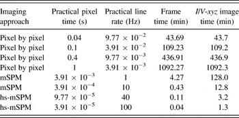
Unfortunately, the precise locations of I–V spectra acquired pixel by pixel are difficult to synchronize with pre- or post-AFM images and their spatial resolution is inevitably, at best, very pixelated. This is primarily due to the relatively long settling times required when repositioning the AFM probe at each new pixel. Practical times spent per pixel are therefore relatively long compared to continuous scanning by an AFM tip and corresponding multidimensional scanning probe microscopy (mSPM) experiments.Reference Herruzo, Asakawa, Fukuma and Garcia36 For example, the second column of Table I presents pixel times in seconds for a range of parameters for individual spectra or scanning measurements. The fourth row, italicized, indicates the most common settings for a single I–V acquisition (1 voltage cycle per second and hence more than 1000 min for a full 256 × 256 pixel resolution I/V map). The first 3 data rows are based on measurement times per pixel that are more ambitious, but diminishingly feasible. Regardless, the corresponding acquisition times for a complete set of 256 by 256 pixels range from practically long (hours) to essentially unfeasible (full working day). Several disadvantages result, including susceptibility to thermal drift, inaccuracies for positioning actuators (hysteresis and creep), the possibility of sample modification, decay, and oxidation. There is an additional caveat as well, in that images are not simultaneously acquired with the point by point I–V spectra, and hence any sample or tip damage, or imprecision in the actual tip position, cannot be observed and especially corrected in real time.
Representative acquisition times for arrays of conventional (pixel by pixel) I–V spectra (top 4 data rows) acquired at rates ranging from impractical (row 1) to common (row 4), compared to parameters for NCM implementing mSPM with equivalent pixel resolution (last 4 data rows) for standard (row 5) to high-speed scanning (row 8).

These issues can be somewhat mediated by hardware and software solutions. Closed loop positioning in AFM can correct for actuator irregularities, though this cannot mitigate the common issue of independent thermal drift of the sample with respect to the tip. Of course, software-enabled feature tracking could correct for such a drift, if regular image updates were available that is, unfortunately, not the case for pixel-by-pixel I–V spectra. Alternately, specialized systems with high thermal stability are proven for maintaining the tip at a fixed position, demonstrated particularly in atomic scale, ultra-high vacuum (UHV) SPM work.Reference Allers, Schwarz, Schwarz and Wiesendanger37,Reference Albers, Liebmann, Schwendemann, Baykara, Heyde, Salmeron, Altman and Schwarz38 But all of these challenges generally persist for the far more widely used ambient measurements with standard commercial hardware and especially for legacy systems. The most commonly applied solution is therefore simply to acquire fewer I–V spectra in a given area of interest, thus still providing the valuable multidimensional data (x, y, z, I, and V), but with a corresponding (and generally highly deleterious) decrease in spatial resolution.
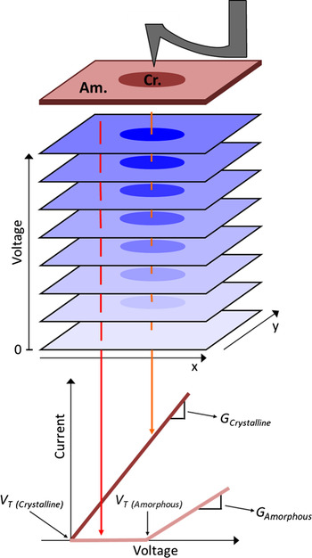
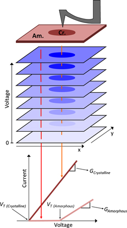
Accordingly, this work acquires high-resolution multidimensional results (still x, y, z, I, and V), but by leveraging the primary forte of AFM, i.e., imaging, instead of a persistent challenge, i.e., parking the tip in a precisely known location. Specifically, numerous consecutive conductive AFM (c-AFM) images are acquired recording current I in the x–y planes, each with distinct voltage V bias, and then the stack of images are reassembled into a 3-d dataset of current versus area and voltage (Fig. 1). The array of I–V curves, 65,536 of them for a standard 256 by 256 pixel stack of c-AFM images, can then easily be used to calculate and map properties for the imaged area with the same nanoscale spatial resolution inherent in the individual images. Voltage resolution is evidently determined by the number of image frames and the voltage span. Crucially, thermal drift problems become practically negligible within any single image as each frame is acquired in seconds to minutes instead of hours to many hours for point by point I–V acquisition. Feature tracking from one image to the next (real time or in postprocessing) can also easily be used, while the tip or specimen damage can be directly observed and coped with in real time. This mSPM approach is therefore particularly suited for investigating nanostructured or heterogeneous electronic materials and devices, where conductivity may differ significantly over the probed area, demonstrated in this work for nanoscale conductance mapping (NCM) as well as simultaneously acquired maps of the “turn-on” switching voltages for micron-sized areas of phase change thin films reflecting nanoscale area phase transitions.
Sketch of NCM for a heterogeneous phase change memory thin film of GeSe. Consecutive c-AFM images are acquired with incrementally higher applied voltages. Current versus voltage (I–V) curves are then extracted for each pixel to efficiently quantify and map local conductance properties.

Of course, similar multidimensional stacks have been used elsewhere, as it is relatively straightforward to automate changes in distinct imaging or sample parameters from one SPM scan to another. For example, phase and amplitude have been recorded during atomic scale AFM imaging, with each frame acquired at a different separation distance, yielding contrast related to the particular atom beneath the tip.Reference Baykara, Schwendemann, Altman and Schwarz39 On a larger scale, multiple acoustic AFM images each with distinct ultrasonic excitation frequencies provided efficient maps of local contact stiffness,Reference Huey40 and recently consecutive friction images with decrementing normal loads yielded maps of the friction coefficient.Reference Bosse, Lee, Huey, Andersen and Sutherland41 Current imaging tunneling spectroscopy (CITS) is the most closely related analog, implemented in STM.Reference Ho42 Since the base platform for the nanoscale conductance mapping (NCM) technique presented here is c-AFM, though, it is much more widely applicable than CITS. This is because it enables high spatial resolution maps of electron transport in specimens with highly insulating regions, not just conductors, of increasing importance for real, nanostructured electronic devices. Furthermore, while NCM is applicable at any scanning speed, with any new or legacy AFM, the results presented here incorporate recent advances in high speed SPM. This enables not just results with negligible thermal drift, but highly efficient image acquisition as well, with obvious benefits for larger area detection, dynamic studies, and high throughput studies.
II. STANDARD CONDUCTANCE MEASUREMENTS
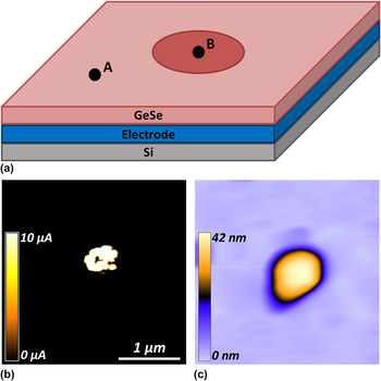
Figure 2(a) exemplifies a common application of AFM-based current studies to a material with nanoscale heterogenous electronic properties. The specimen is a 50-nm-thick amorphous GeSe layer, grown by thermal coevaporation on an underlying conducting back electrode of PtReference Jeong, Lim, Park, Hwang, Lee and Cheong43 with a Si substrate. The GeSe film was determined to have the composition of Ge51Se49 (in at. %) from the electron probe x-ray microanalysis. The specimen contains both amorphous and crystalline phases, as shown in the topography (b) image, and a corresponding current map acquired while simply continuously biasing the scanned probe with 1.3V DC (c).
Sketch (a), AFM topography image (b), and standard c-AFM current image (c) of a model phase change specimen with a crystalline “bit” (B) at the center of an amorphous (A) GeSe film.

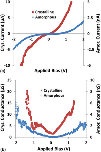
Figure 3(a) presents standard c-AFM I–V curves acquired from a similar amorphous and crystalline region of the GeSe film, locations (A) and (B) respectively, as indicated in Fig. 2(a). Both of the I–V curves were acquired by positioning the tip somewhere in the distinct specimen regions, then ramping the voltage from −2 to +2 V and back with 5 mV steps at a cycle rate of 1 Hz. The current is sampled every millisecond, providing 500 current measurements in each direction. Note that the y-axes are in microsiemens for the crystalline I–V spectra and in nanosiemens for the amorphous location due to the profound difference in conductivity. The highly conducting crystalline phase actually reaches the upper and lower current acquisition limits (±10 µA) of the c-AFM at +1.31 and −1.60 V, respectively. Conversely, the current measured at the amorphous phase was typically 4 orders of magnitude less throughout the experiment. Imaging and acquiring I–V spectra and/or topographic images for such disparate phases with STM and/or CITS would be extraordinarily challenging, but with c-AFM, it is thus relatively straightforward.
Standard I–V curves acquired at typical pixel-by-pixel rates (1 Hz) on crystalline and amorphous regions of a GeSe phase change film (a, note distinct scales at left and right). The conductance has also been calculated (b) for the crystalline and amorphous regions, respectively, revealing differences of 4 orders of magnitude (note scale difference).

The slope of the I–V curve is used to calculate the conductance at any applied voltage for both crystalline and amorphous phases [Fig. 3(b)]. Due to conductance on the crystalline bit of almost 4 orders of magnitude greater than that on the amorphous region, a maximum measured conductance for the crystalline phase of 20.30 µS at −1.44 V versus 5.26 nS at −1.94 V for the amorphous phase.
III. NANOSCALE CONDUCTANCE MAPPING
The obvious challenge with simple I–V spectra as in Fig. 3 is that to spatially resolve nanoscale specimen features, many hours are required to sequentially collect thousands of closely packed voltage sweeps, as exemplified in Table I. When implementing the mSPM technique for conductance mapping, on the other hand, the tip is simply continuously scanned, while the voltage is changed only occasionally and subtly (e.g., at the start of each new frame, by a small ∆V). Settling times are therefore completely avoided, providing extensive benefits even at moderate scanning speeds. For example, a single image frame when scanning with a 10-Hz line rate (Table I, data row 6) requires 25.6 s (0.43 min, data column 3), providing a full spatial resolution I/V-xyz map in only ∼13 min for 30 consecutive images or voltage steps (data column 4). This is compared to 109.2 min (1.8 h) for an extremely difficult to achieve rate of 10 pixels/second of I–V spectra (data row 2). Using recent advances in high-speed SPM,Reference Picco, Bozec, Ulcinas, Engledew, Antognozzi, Horton and Miles44 with line scanning rates up to thousands of Hertz, allows even more impressive enhancements, requiring just 7.7 s at 1 kHz line rates for a sequence of 30 images, or 1.3 min at a more commonly manageable 100 Hz scanning rate, such that high spatial and voltage resolution I/V data is achieved by NCM.
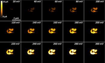
Figure 4 displays a montage of 15 such c-AFM images extracted from a sequence of 30 consecutive scans, each with incremented voltages from 10 mV up to 300 mV as indicated. All of the frames are acquired in the same 1.5 × 1.5 µm area, with a moderate 10-Hz line scan rate equivalent to spending 391 µs per pixel. Collectively this amounts to just 12.8 min to acquire all 65,536 I–V spectra with 30 voltage steps each. This amounts to an 85x improvement when compared to the 1-Hz acquisition rate for a single pixel as displayed in Fig. 3. To put this into a better perspective, the 13-min NCM experiment would require more than 18 h to equivalently complete with traditional point by point I–V mapping.
Montage of current images at distinct applied voltages as labeled, representing a subset of 30 total frames for the same 1.5 × 1.5 µm area, all imaged at a line rate of 10 Hz. The field of view displays a conducting crystalline region in an otherwise amorphous GeSe thin film.

Despite the minimal spatial drift offered by this higher speed approach compared to pixel-by-pixel based spectra, image-by-image drift naturally still occurs, at least to some extent. Therefore, before assembling I–V curves by stacking the frames of Fig. 4, simultaneously acquired topographic data is used to align the individual frames based on image correlation functions in standard image processing software (e.g., ImageJ, NIH). The positions of each frame are consequently slightly shifted in x and/or y directions as needed, in this case, by a maximum of 60 and 6 nm for the fast and slow scan directions, respectively. Practically, any locations that are not imaged in every single frame are truncated from the final results, typically representing a few percent of image pixels around the image periphery (of course depending on the magnitude and direction of lateral drift throughout the experiment). Furthermore, such drift could also be minimized by real-time scanning corrections with suitable software and closed loop scanners.
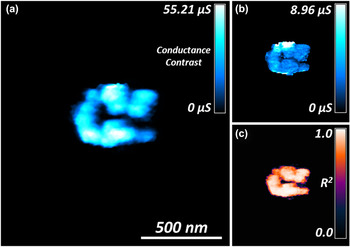
After such a drift correction, the matrix of acquired I–V curves can be used to map a variety of transport properties for the specimen, providing both nanoscale spatial resolution, as well as high confidence in the positional accuracy of the corresponding I–V results. For example, a map of the conductance can be calculated by fitting the shape of each I–V curve, Fig. 5(a), with pixel dimensions here of just 6 × 6 nm. Consistent with the standard current image of Fig. 2(b), a higher conductivity is apparent in Fig. 5(a) for the central crystalline bit as compared to the surrounding amorphous film. The random scatter in each I–V curve used to calculate the conductance is quantified in Figs. 5(b) and 5(c), which respectively present the 95% confidence error and the coefficients of determination (R 2) for the conductance map. On average, the 95% confidence error amounts for less than 15% of the calculated conductance values. The average coefficient of determination for the conducting bit is 0.88 ± 0.11, clearly confirming the ohmic nature of the I/V response within the crystalline region over the voltage range considered (0–300 mV). However, other I–V relationships in the event of Schottky, thermionic, tunneling, or spin dependent conditions, could alternately be calculated, providing corresponding maps of such features of more complex local materials behavior.
1.39 × 1.49 µm map of conductance resolved down to 6 × 6 nm, based on 60,672 I–V curves from the dataset of Fig. 4, all acquired by SPM in <13 min (a). The corresponding 95% confidence interval is also mapped (b), as is the coefficient of determination, R 2, for the measured conductance (c).

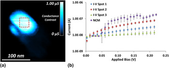
The acquired current with standard I–V spectra has been compared to the NCM method (Fig. 6). I–V curves were acquired at ten spots on the crystalline bit. All ten I–V measurements were acquired within the marked dashed box of Fig. 6(a). However, seven of the ten measurements were at the noise floor of the current detector, indicating that thermal drift pushed the probe into the amorphous region. The three I–V measurements with an appreciable current signal (true position on the crystalline bit) are presented as I–V spot 1, 2, and 3 in the legend of Fig. 6(b). Subsequent imaging was performed to construct the conductance map in Fig. 6(a). The average conductances of the three standard I–V curves in Fig. 6(b) are 112 ± 28, 333 ± 44, and 29 ± 18 nS. The average conductance of the I–V curve extracted from the NCM method is 605 ± 187 nS.
Subset of 312 × 329 nm map of conductance calculated from 23 c-AFM images with a line scan rate of 10 Hz (a). Images were acquired from 0 to 220 mV bias with 10 mV steps. Current versus applied bias for standard I–V curves and NCM extracted I–V curve of the crystalline bit (b). Standard I–V curves were acquired from −2 to +2 V with 3 cycles at a 3 Hz ramp rate. The NCM I–V curve is an average of 20 × 20 pixels from the box in (a).

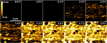
Due to the ∼4 order of magnitude difference in conductance between the crystalline and amorphous phases, it was impractical to simultaneously resolve both the subtle conductivity variations within the amorphous phase, and the maximum conductivity in the crystalline phase. Separate results have thus been acquired in the same manner, but with the current detector set at its highest sensitivity (5 pA–10 nA), to investigate the amorphous phase of the GeSe film alone, with no crystalline bit present. Figure 7 displays a montage of 10 c-AFM images extracted from a complete sequence of 19 consecutive scans, each with incremented voltages from 0 to 3.6 V (only those up to 1.8 V are shown). All images have been acquired from the same 4 × 4 µm region. A modest 10-Hz line scan rate was implemented for all acquired images, as with Fig. 4. The total linear drift was just 16 and 86 nm in the fast and slow scan directions, respectively, leading to a final conductance map with 65,280 points (237 by 254 pixels).
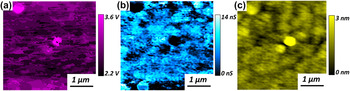
Interestingly, unlike the crystalline phase, we found that the amorphous phase does not conduct current appreciably until a spatially dependent threshold turn-on voltage is reached [Fig. 8(a)]. This turn-on voltage is characteristic of the traditional semiconductor behaviorReference Cowley45,Reference Card and Rhoderick46 and is easily determined from the I–V curves extracted from each pixel of Fig. 7. Figure 8(b) displays a map of the corresponding conductance map of the amorphous GeSe film, calculated based on the I–V slope beyond the turn-on voltage only (thus avoiding artificial offsets in the conductance due to varying turn-on potentials). As suggested by the early frames in Fig. 7 montage, the turn-on voltage can be as low as 1.1 V within the amorphous film. For some regions, however, no current was detected even during the maximum applied bias of 3.6 V, indicating an even stronger local turn-on voltage. This ability to map local electronic transport is clearly important for applications such as resistive or phase change data storage systems, where uniformity from one nanoscale bit to another will be crucial in terms of ultimate operating speeds, power requirements, and reliability.
Montage of current images at distinct applied voltages as labeled, representing a subset of 19 total frames for the same 4.0 × 4.0 µm area, all imaged at a line rate of 10 Hz. The field of view displays the amorphous GeSe thin film with no crystalline bit present.

3.98 × 3.83 µm map of the turn-on voltage for an amorphous GeSe film, based on 65,280 I–V curves from the dataset of Fig. 6, all acquired by SPM in just 8 min (a). The corresponding conductance (b) and topography (c) is also shown, resolved down to 16 × 16 nm.

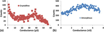
Of course, such a spatial resolution might not be achieved using traditional I–V methods, in which case, the mean response of many I–V spectra, and/or a histogram, would typically be reported. Similar histograms from the NCM conductance maps are shown for the crystalline, and separately the amorphous phases [Figs. 9(a) and 9(b)]. The mean conductance for the crystalline region alone in Fig. 5(a) is 25.0 ± 15.9 µS, whereas that for the amorphous film in Fig. 8 is 5.0 ± 2.9 nS. As expected from the standard I–V curve measurements, the crystalline phase has a conductance that is more than 3 orders of magnitude higher than the amorphous phase. As with all histogram analyses, the relative ratio and distribution of properties can thus be visualized, for example, to assess a relative areal fraction of switched material when normalized by the analyzed area. With the new NCM approach presented here, though, such distributions of conductivity behavior can now also be precisely coupled spatially to various nanoscale specimen features, providing valuable benefits for heterogeneous specimens in general.

IV. CONDUCTANCE MAPPING ARTIFACTS
While applying the NCM approach as well as any of the other AFM-based current measurement schemes, there are several possible artifacts that one must consider. First, it is critical that the tip maintains a constant applied normal load (i.e., contact or setpoint force). Varying this applied normal load from location to location could cause the contact area to change,Reference Huey40 possibly causing the detected current to shift higher or lower than anticipatedReference Dewolf, Snauwaert, Clarysse, Vandervorst and Hellemans3 especially if the correlation between contact area and current is nonlinear.Reference Keenan, Schumann, Tong and Phillips47,Reference Henisch48 Even more critical, though, is that this constant force should be both high enough to produce a consistent current measurement (generally sufficient to push through any surface contamination) while remaining reasonable such that the tip and/or specimen are not plastically deformed or modified. Fortunately, negligible variations in image quality and feature size/shape have been documented over each set of images on the GeSe film. This suggests that the scanning conditions are stable and nondestructive. These conditions are apparent in the consecutive images depicted in Figs. 4 and 7, as sub-20 nm features are consistently resolved.
The second possible common artifact is due to changes in contact area during scanning related to topographic features or regions with dramatically different mechanical properties. This latter concern is negligible for the GeSe specimens considered here, as the amorphous and crystalline regions are uniformly stiff versus the comparatively compliant AFM probe. With polymer specimens, however, such variations must rigorously be accounted for. General topographic variations, on the other hand, are ubiquitous in AFM imaging, most apparent here when comparing the amorphous GeSe current maps of Fig. 7 with the local topography [Fig. 8(c)]. Areas with higher topography consistently display a lower current then their lower topographic counterparts, likely due to the decreased contact area between the tip and local convex surface. Consistent with this observation, local areas of the sample that are concave with spatial dimensions similar to the probe tend to display a higher relative measured current. These contact area effects are unavoidable in I–V detection and c-AFM but can be diminished by utilizing sharper AFM probes.
The third potential artifact with current or conductance mapping concerns specimen stability. Certain specimens are susceptible to oxidation, thermal variations, and humidity (or lack thereof). The water meniscus that develops at the tip sample junction for ambient measurements influences current measurements as well via the relative contact areaReference Weisenhorn, Maivald, Butt and Hansma49 and can even lead to electrochemical reactions. The efficient frame-by-frame approach of NCM, especially if leveraging high speed SPM, minimizes this issue by making the measurements faster (with less time for oxidation or humidity variations to intercede). Moreover, any specimen changes that do occur due to the environment negligibly influence the I–V response from one pixel to another, since the sample state is essentially identical for every single pixel for a single image (at a single voltage). Of course, such environmental effects can still shift the magnitude of the measured current for every pixel in any given image (voltage), with the current response for the final image frames sampling a possibly environmentally damaged surface while the initial specimen may be pristine. If such a “drift” in the environmental response is uniform, though, then it can easily be corrected. Moreover, it is trivial to test for such effects by comparing single I–V spectra acquired before and after NCM maps. Pixel-by-pixel spectra, on the other hand, can be extremely problematic in such circumstances since the first pixel measured at one corner of an area may be for an ideal specimen, whereas the last pixel from the opposite corner may be after substantial specimen degradation, requiring much more challenging pixel-dependent corrections. Regardless, to alleviate any such artifacts for the results presented here on GeSe films, all data were acquired while the experimental chamber was continuously purged with Argon.
In a related sense, simple voltage sweeps can be damaging to the region beneath the probe for some specimens, possibly influencing nearby regions as well through percolation paths, charging, or even breakdown events. Scanned instead of pixel-by-pixel I–V data therefore present an additional benefit, for example, through images with consecutively stronger voltages because any breakdown events at certain pixels do not completely hinder future I–V spectra for adjacent pixel measurements—spectra for all pixels (at least to the same maximum voltage) have already been acquired. NCM results are correspondingly more comparable to macroscopic I–V measurements of practical devices, where the ensemble behavior of adjacent regions, especially their interrelated response, defines the overall device properties.
Since updated topographic and current maps are continuously acquired with NCM, the influence of any of the artifacts discussed above can additionally be observed in real time. Experimental parameters can then easily be corrected, measurements restarted, or details modified. Sample, tip, or system problems are substantially more difficult to identify and/or correct during consecutive pixel-by-pixel acquisition of I–V spectra.
V. CONCLUSION
NCM is an important tool for efficiently mapping electronic transport in heterogeneous materials with nanoscale resolution. It is inherently more efficient than pixel-by-pixel I–V acquisition schemes, particularly when implementing leveraging high-speed SPM. Here, it is used to map electron transport for crystalline and amorphous phases of a GeSe phase change film. As confirmed with single I–V spectra, the mapped conductance for the crystalline phase is more than 3 orders of magnitude stronger than the amorphous phase. Meanwhile, the amorphous region exhibits variations in conductance, and separately an effective turn-on voltage, that are spatially independent. NCM is therefore promising for investigating the influence of phases, defects, interfaces, and/or topographic features on electronic transport in heterogeneous materials, particularly those with highly varying conductivity regions such as MEMS/NEMS devices, phase change memories, and nanostructured photovoltaics.
VI. EXPERIMENTAL
All experiments are performed at room temperature with an Asylum Research Cypher AFM (Santa Barbara, CA). The specimen is enclosed in the scanning chamber with a constant flow of argon gas at 20 CFH to minimize specimen oxidation and provide a constant water meniscus at the tip/specimen junction. Current detection is performed with an Asylum Research ORCA cantilever holder that features a dual gain current sensitivity of 1 µA/V (low gain) and 1 nA/V (high gain). The current resolution for the low and high gain is 1 nA and 5 pA, respectively.
Diamond-coated silicon cantilevers (Nanosensors, CDTP-NCHR) are used throughout, with a quoted tip length of 10–15 µm, a cantilever length of 125 ± 10 µm, and a resonant frequency of 275–720 kHz.
The amorphous GeSe film was prepared by chemical vapor deposition in a plasma discharge stainless steel reactor on a conducting back electrode. Both the amorphous GeSe film and the back electrode were deposited on a silicon wafer for mechanical stability. A low-pressure plasma was created by an rf discharge between two parallel plate electrodes, where both silicon substrates were fixed. The precursor gases used for the deposition were GeH4 and H2Se, and deposition was continued until a GeSe film thickness of 50 nm.Reference Márquez, Nagels, González-Leal, Bernal-Oliva, Sleeckx and Callaerts50
For the turn-on voltage map of the amorphous GeSe film in Fig. 7(a), the calculated threshold voltage corresponds to when the current rises above 100 pA. This is approximately 20 times higher than the noise floor of the high gain detector.
ACKNOWLEDGMENTS
BDH appreciates support from the Velux Foundation and iNANO, JB from NSF:DMR:Ceramics, 0909091, and SL from NSF:DMR:IMR, 0817263, OVK acknowledges the support from the EPSRC-NSF grant EP/G06556X/1 and EU grant FUNPROB.