INTRODUCTION
The management of land for food production is a fundamental human activity. From the 14 billion ha of ice-free land on Earth, 0·10 is used for crop cultivation, and an additional 0·25 is used for pasture (Tubiello et al. Reference Tubiello, Soussana and Howden2007). The productivity of crops is determined by a set of yield defining factors (e.g. climate, atmospheric CO2 concentration and crop characteristics), limiting factors (e.g. water and nitrogen supply) and restricting factors (e.g. pest and diseases) (Goudriaan & Zadoks Reference Goudriaan and Zadoks1995). Oerke & Dehne (Reference Oerke and Dehne1997) estimated that the worldwide control of disease reduces potential yield losses by 23%. However, animal pests and weeds can reduce potential yield by 31 and 55%, respectively. Weeds can be controlled by chemicals, mechanical means or by hand weeding and efficiently reduces potential yield losses by 50%. Crop protection against yield limiting factors can reduce potential yield losses by more than 70%, which demonstrates the potential of modern crop protection practices.
Weather fluctuations are known to influence the population dynamics of many insect species (Griebeler & Gottschalk Reference Griebeler and Gottschalk2000). The present study considers three insect species whose development depends on temperature and other climatic conditions: the European corn borer (Ostrinia nubilalis), European grape vine moth (Lobesia botrana) and Codling moth (Cydia pomonella).
The efficiency of pest management programmes depends on the treatment of the pest populations at their most susceptible stage. Control treatments commonly rely on either pheromone traps that catch pests or temperature sums. Another frequently used method is life stage modelling, which is often performed based on accumulated degree-days. The approach of degree-days is justifiable, especially for C. pomonella, because the most important natural factor for its development is air temperature (Neamtu et al. Reference Neamtu, Barbulescu, Petrisor, Stinga, Cornel, Drosu, Chireceanu, Ioan and Cristian2008). The degree-days method is also involved in the phenological model for C. pomonella that was developed by Boivin et al. (Reference Boivin, Chadoeuf, Bouvier, Beslay and Sauphanor2005). Sophisticated simulation models such as the Bugoff 2, which was developed especially for determining the time of application for the C. pomonella granulosis virus, are rarely used by practical advisory services. Bugoff 2 can determine the hatching rate of the codling moth under field conditions (Blago & Dickler Reference Blago and Dickler1990). Another forecasting tool is SOPRA, which was developed and used in Switzerland to optimize control measures for various insect pests in orchards (Graf et al. Reference Graf, Höpli and Höhn2003). Milonas et al. (Reference Milonas, Savopoulou-Soultani and Stavridis2001) used a degree-days model to forecast the first appearance of L. botrana in field conditions and to monitor their flight activity. Moravie et al. (Reference Moravie, Davison, Pasquier and Charmillot2006) mentions a model that estimates the most appropriate time for applying pheromone confusion or chemical treatments for L. botrana based on insect emergence time. A mathematical model of the temperature-dependent development of arthropods was used by Briere et al. (Reference Briere, Pracros, Le Roux and Pierre1999). This model was applied to compare the developmental rates of L. botrana at constant temperatures.
Several studies that deal with O. nubilalis development are closely related to meteorological conditions during a given season (Trnka et al. Reference Trnka, Muška, Semerádová, Dubrovský, Kocmánková and Žalud2007; Kocmánková et al. Reference Kocmánková, Trnka, Žalud, Semerádová, Dubrovský, Muška and Možný2008). Beyond temperature, the biological cycle of the pest is affected by the length of day, scotophase (defined here as the period when the sun is 6° or more below the horizon) and latitude (Onstad & Brewer Reference Onstad and Brewer1996). Induction of diapause is also considered to be determined by photoperiod in other two species (C. pomonella and L. botrana): Casada González (Reference Casada González2007) suggests that the combination of day-length of 15·25 h and temperatures of 25 °C affects induction of diapause in C. pomonella. Photoperiod is the second most important factor affecting both the number of L. botrana generations completed in a year and the number of pupae entering diapause (Gabel & Mocko Reference Gabel and Mocko1984). The critical diapause-inducing photoperiod for L. botrana is c. 13 h at 25–26 °C; while a longer photoperiod at a constant colder temperature (22 °C) did not induce diapause. Under field conditions, the photoperiod necessary to induce diapause was c. 15 h (Deseo et al. Reference Deseo, Marani, Brunelli and Bertaccini1981).
The dependency of O. nubilalis development on climatic conditions makes O. nubilalis suitable for climate-driven modelling that estimates species population dynamics and occurrence. An assessment of climate favourability for the univoltine and bivoltine populations of the European corn borer has previously been performed using the ECAMON model (Trnka et al. Reference Trnka, Muška, Semerádová, Dubrovský, Kocmánková and Žalud2007).
The aim of the present study was to investigate how climatic variability during the period 1803–2008 affected the climatic niches of potential pests. This assessment was completed independently of the historically observed occurrence of the nominated pests. In addition to estimating the climatic suitability for the persistence of a given pest in the past, another aim of the study was to specify the core climatic niche with continued pest presence. Furthermore, the applicability of the generated meteorological data for climate change based on pest mapping was evaluated. Simulations were based on developmental biological parameters obtained from the literature, and were altered during model calibration. This approach agrees with the methodology of the climate-matching software, CLIMEX, which was used in the present study.
MATERIALS AND METHODS
The first pest investigated in the present study was the European corn borer (O. nubilalis), which is native to Europe and is the most important pest impacting maize (Zea mays). Evidence of the harmful occurrence of O. nubilalis in the Czech Republic dates back to 1879, when it was a significant pest of hop plants (Kapler et al. Reference Kapler, Picková and Pražan2007). In the 1950s, O. nubilalis impacted maize production in the south Moravia region but recently summaries by the State Phytosanitary Administration (SPA), which are conducted every 10 years, have shown that it has spread to other regions of the Czech Republic too (Kapler et al. Reference Kapler, Picková and Pražan2007). In addition to host plant abundance, local climatic conditions and weather patterns within a given growing season are the dominant factors that determine the intensity and occurrence of O. nubilalis. In particular, temperature determines the length of the life-cycle and, consequently, the number of generations completed.
The second pest investigated was the codling moth (C. pomonella). This is the oldest known and most widely distributed pest of deciduous pome fruit (Ferro & Harwood Reference Ferro and Harwood1973). The native home of the codling moth is south-eastern Europe; however, it has spread to various parts of the world and now occurs in temperate regions on all major continents. In addition, it has demonstrated an ability to colonize apple and pear trees in regions where the climate is suitable for commercial production. It is evident that the present distribution of the codling moth is related to both climatic factors and the distribution of the host species (Wearing et al. Reference Wearing, Hansen, Whyte, Miller and Brown2001).
The third pest investigated was the European grapevine moth (L. botrana), which is also native to Europe. It was first described in Vienna in 1775 by the biologists Denis and Schiffermüller from samples collected in Italy, and was classified as a pest in Austria in 1800 (Varela et al. Reference Varela, Smith, Cooper and Hoenish2010). Lobesia botrana, together with the grape berry moth Eupoecilia ambiguella, is the dominant pest in European vineyards and causes damage to vines by feeding on flower buds and berries while in its larval stages. Processes such as fecundity, survival and development rates are involved in moth population dynamics (Moravie et al. Reference Moravie, Davison, Pasquier and Charmillot2006) and can be influenced by ecological factors, such as temperature, humidity and food quality.
CLIMEX (CLIMatic indeEX) is a simplified computer model that infers the response of a species or biological entity to climate by using its geographical distribution, its seasonal growth pattern and its mortality in different locations (Beddow et al. Reference Beddow, Kriticos, Pardey and Sutherst2010). CLIMEX is a climate-driven modelling program that is designed to provide insight into the climatic requirements of a species, as expressed by their geographical distribution, seasonal phenology and relative abundance. The CLIMEX program assumes that it is possible to define climates that are favourable for the generation of particular weather patterns, which directly affect populations on a short time-scale (Sutherst Reference Sutherst, Mooney and Hobbs2000a). The program derives weekly and annual indices that describe the responses of a given species to changes in temperature, moisture and (in the case of plants) light (Sutherst Reference Sutherst2003). These properties make CLIMEX an appropriate tool for planning questions about risk assessment issues in integrated pest management and quarantine, biological control or climatic variability and long-term climate change (Sutherst Reference Sutherst, Hammer, Nicholls and Mitchell2000b).
Knowing the climatological requirements of a given species allows assessment of the suitability of an area for population growth and to determine the stress induced by unsuitable climate conditions. These factors are expressed by the ecoclimatic index (EI), which describes the overall suitability of climate conditions for the establishment and long-term presence of a pest population at a given location:
 $${\rm EI} = {\rm GI}_{\rm A} \times {\rm SI} \times {\rm SX}$$
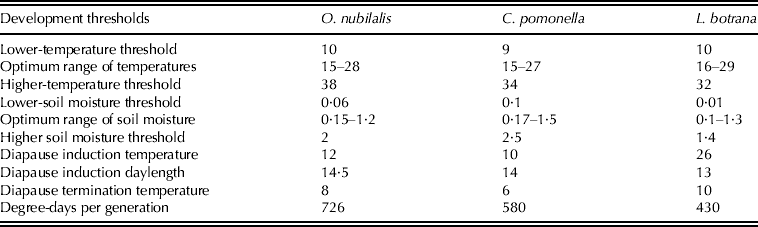
where GIA is the annual growth index describing population growth under favourable conditions, SI is the annual stress index describing survival during unfavourable periods, and SX is a measure of stress interactions. Calculation of the GIA and stress indices is based on the ranges of the threshold parameters for species development and adjusted by the user (Table 1). The temperature parameters include the upper and lower thresholds and the optimal range of air temperature for development. Similar parameters are also used for soil moisture. In addition to the temperature and moisture limitations, CLIMEX also accounts for the process of diapause, which is driven by temperature (initiation and termination temperature) and day-length thresholds. The number of pest generations is calculated based on the number of degree-days above the lower temperature threshold for each generation. Generally, EI ranges from 0 to 100, where EI=0 indicates climatic conditions that are unfavourable for long-term species occurrence and EI >30 represents very suitable climatic conditions for species occurrence (Sutherst & Maywald Reference Sutherst and Maywald1985). Hoddle (Reference Hoddle2004) considers locations with EI>25 as very favourable for species occurrence, locations with 10<EI<25 as favourable and locations with EI<10 as limiting for species survival and occurrence. The CLIMEX model uses input data on a monthly scale (minimum and maximum temperatures, relative humidity at 09·00 h and 15·00 h and precipitation).
The temperature (°C), daylength (h), and moisture developmental thresholds of O. nubilalis, C. pomonella and L. botrana. The moisture threshold is a combination of two parameters: (i) soil moisture storage capacity (default 100 mm representing a soil profile with a depth of c. 500 mm and a moderate water-holding capacity) and (ii) evapotranspiration coefficient (default value is 0·8 typical for mature pasture/crop areas). Soil moisture of 0·1 indicates soil moisture content is 10%. Soil moisture >1 indicates water content greater than the soil-holding capacity of i.e. run-off (see Sutherst et al. Reference Sutherst, Maywald, Bottomley and Bourne2004)

Reliability tests of the modelled establishment of a particular pest were used with developmental thresholds taken from the literature (Table 1). The modelled pest presence was verified by comparing the observed pest occurrence with the number of generations in a given modelled area. Model parameters were then altered to truly describe the pest presence. The model was tested for C. pomonella and O. nubilalis in the central European domain using the 1961–1990 reference period (Kocmánková et al. Reference Kocmánková, Trnka, Eitzinger, Dubrovský, Štěpánek, Semerádová, Balek, Skalák, Farda, Juroch and Žalud2011; Svobodová et al. Reference Svobodová, Trnka, Žalud, Semerádová, Dubrovský and Šefrová2011). The L. botrana model along with its reliability test is described in the present paper. Model verification took into account the harmfulness of L. botrana throughout Europe and the number of L. botrana generations in several European countries (Fig. 1). The model simulation used climatic data that represented the period from 1961 to 2000.
(Colour online) The reliability test of the L. botrana model is shown here. Visualization of the ecoclimatic index that represents the favourableness of climates for the development of one (green), two (yellow), three (orange) or four (red) generations of L. botrana. Blue represents areas without presence of the pest. Red circles mark the observed occurrences of the pest from the database of the Fauna Europea and the Suffolk Moth Group. The yellow line constitutes the potential northern range that was estimated based on the CLIMEX model results.
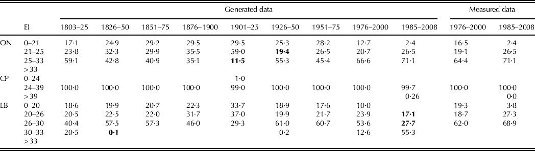
Following model verification and calibration, meteorological data were altered to represent the meteorological series climatic conditions from 1803 to 2008. These data had two forms: firstly, the meteorological series that was generated for the 1803–2000 period was used in six separate simulations in time-steps of roughly 25 years and secondly the 1985–2008 period. The exact structure of modelling periods regarding to generated and measured meteorological data are shown in Table 2.
The ratio of arable land that is affected by a particular pest's generation (in terms of EI ranges) according to simulations using generated meteorological data and measured meteorological data in particular periods. Bold values constitute the climatic niche core area (ON: Ostrinia nubilalis, CP: Cydia pomonella, LB: Lobesia botrana)
To produce a meteorological series that represented past climatic conditions for the study area, a stochastic weather generator (Met & Roll) (Dubrovský et al. Reference Dubrovský, Buchtele and Žalud2004) was focused on high-quality daily observations from 52 representative meteorological stations during the baseline period (1961–1990). Therefore, an approach was applied that has been used routinely in climate change studies (Trnka et al. Reference Trnka, Dubrovský and Žalud2004).
The measured meteorological series for the 1976–2008 period was divided into two sub-periods (1976–2000 and 1985–2008). Therefore, the first 25 year period from 1976 to 2000 refers to the identical semifinal period of generated data while the period from 1985 to 2008, as in the case of the generated data, represents the final warmer period of the 20th–21st centuries.
Both generated and measured meteorological data were applied for 52 representative meteorological stations in the southeast Czech Republic and the northern Austria regions (Fig. 2a). Simulation outputs were visualized using Geographical Information Systems (GIS) with a digital landscape model (grid layer with resolution of 1×1 km).
(Colour online) Map of the region involved in the model. (a) marked stations constitute detailed geographical position of C. pomonella simulation results: 1–Krems, 2–Laa Thaya, 3–St. Pöelten, 4–Wien, 5–Wörtenberg, 6–Pohořelice, 7–Strážnice, 8–Velké Pavlovice. The coloured scale depicts the annual mean temperature and represents the 1961–2000 period. (b) land use in the region.
RESULTS
European corn borer (O. nubilalis)
The corn borer develops one or (in rare cases) two partial generations in the Czech Republic and Austria (Bírová et al. Reference Bírová, Brestovský, Jakubčin and Longauerová1990). The modelled occurrence of the corn borer using the generated meteorological data resulted in the persistence of the first generation corn borers (EI 21–25) in the largest arable land area at the beginning of 20th century (0·59 during the period 1901–1925). In addition, a partial second generation (EI 25–33) occurred in the period 1985–2000 (0·71 of arable land), which agrees with field observations and supports the link between corn borer reproduction and increasing temperatures. The progress of infestations across the arable land by particular generations is shown in Table 2. In Fig. 3, the infested regions are depicted regardless of the acreage of maize cultivation. In addition, Fig. 3 shows the minimum area of the first and partial second generations, which are actually the cores of the climatic niches. The geographical position of the first generation climatic niche is visible in the 1951–1975 map, which shows the core of the climatic niche for the first generation in the relatively wide and stable (in terms of size) areas of southern Moravia and northern Austria. The determination of this area is crucial, because a continuous O. nubilalis first generation presence corresponds with the long-term establishment of the pest that was estimated in the model validation by Kocmánková et al. (Reference Kocmánková, Trnka, Eitzinger, Dubrovský, Štěpánek, Semerádová, Balek, Skalák, Farda, Juroch and Žalud2011). The core of the climatic niche for the partial second generation can be seen in the 1901–1925 period map and covers the most southern promontory of the Moravia region and the adjacent northward lowland (Fig. 3). In Austria, the climatic niche involves a more extensive area, occupying the entire eastern part (Burgenland) and continuing as far west as Krems (geographical position of Krems location is depicted in Figs 2(a), part (b) show this in the connection of land use).
(Colour online) The simulated distribution of O. nubilalis based on (a) measured and (b) generated meteorological data in different periods. There is an apparent shift in the primary area established by the O. nubilalis first (green) and a partial second (yellow) generations. Blue represents areas without presence of the pest.
The modelled results from the generated and measured meteorological data were similar, which suggests that both models considered the overall region regardless of agricultural land use (Fig. 3). The only significant difference was recorded in the first modelled period from 1976 to 2000, when the partial second generation covered less area in the most northern lowland of the Moravia region. The second difference was that first generation infestations were not found in the north-eastern part of the area when using measured meteorological data, but were when generated data was used. Overall, comparing the ratio of the arable land infested by one generation to the arable land infested by a partial second generation in the 1985–2008 period yielded identical results (Table 2).
European grapevine moth (L. botrana)
The larvae of L. botrana feed on grapevine flowers and berries, and facultative diapause and number of generations per year depend on temperature and photoperiod (Pavan et al. Reference Pavan, Floreani, Barro, Zandigiacomo and Dalla Monta2010). Previous literature suggests that there are greater numbers of L. botrana generations in southern latitudes than in northern latitudes. In addition, two generations of L. botrana occur in the colder areas of Europe, and three generations typically occur in the southern areas of Europe. Up to four generations can occur in warmer regions such as Greece (Moschos et al. Reference Moschos, Broumas, Souliotis, Tsourgianni and Kapothanassi1998). Furthermore, two or three generations typically occur in Germany (Louis et al. Reference Louis, Schmidt-Tiedemann and Schirra2002).
The reliability of the L. botrana model in the European domain was assessed with the CRU TS 1.2 (New et al. Reference New, Hulme and Jones2000; Mitchell et al. Reference Mitchell, Carter, Jones, Hulme and New2003) data for the current climate (1961–2000) (Fig. 1). Simulations using the CLIMEX model have estimated the suitability of climatic conditions for completing a number of generations in the European countries mentioned above. However, there were some inaccuracies in the previous simulations using CLIMEX. For example, there was a disagreement between the modelled L. botrana occurrence and the pest presence in Poland according to CABI (CABI Distribution Maps of Plant Pests, www.cabi.org). However, Fauna Europea (www.faunaeur.org) indicated levels of moth survival in Poland that were in agreement with the CLIMEX model. In addition, the potential presence of L. botrana in Poland is supported by the fact that Poland manages 250–300 ha of vineyards (Lisek Reference Lisek2008) and the HUGLIN Index for wine shows an extension of the potential growing area for grapes in Poland and Northern Europe (Eitzinger et al. Reference Eitzinger, Kersebaum and Formayer2009). In another disagreement relevant to Scandinavia, both CABI and Fauna Europea indicate that L. botrana is absent in Norway, Denmark and Finland, while the CLIMEX model marks Denmark and the southern border of Sweden and Finland as the northern limits for the occurrence of L. botrana, which is in agreement with the HUGLIN index for potential wine growing areas in Europe. The CLIMEX model also correctly indicates the climatic suitability of Gotland, Sweden for this pest (moth presence has been recorded by Fauna Europea). In Denmark and Finland, L. botrana is currently present in glasshouses (Canadian Food Inspection Agency, www.inspection.gc.ca). In the UK, where L. botrana is a rare immigrant in Suffolk (web site of the Suffolk Moth Group, www.suffolkmoths.org.uk), the CLIMEX model results supported this claim.
Meteorological data derived from the generated data set showed a change in the presence of L. botrana during various periods. The changing area of arable land that had one (EI 20·0–25·9), two (EI 26·0–29·9) and three (EI 30·0–32·9) pest generations within a particular period is shown in Table 2. It is clear that the climate niche of L. botrana was greatest during the 1985–2008 period, when the first generation covers the entire modelled domain (Fig. 4). This period was characterized by the warmest climatic conditions. In addition, it allowed the expansion of the third generation of L. botrana, which was recorded in significant areas in three simulated periods (1803–1825, 1976–2000 and 1985–2008). The 1826–1850 and 1926–1950 periods demonstrated only trace areas suitable for third generation L. botrana. If it is assumed that the southern Moravia area and the northern part of Austria are joined, the third generation climatic core occurs in the most southern part of the modelled region in Austria (in Burgenland, the districts ranging from Neusiedl am See and Eisenstadt). This result is shown in the 1826–1850 period map (Fig. 4a). The core of the first and second generation climatic niches is shown in the 1901–1925 period map (Fig. 4a).
(Colour online) The simulated distribution of L. botrana based on (a) measured and (b) generated meteorological data in different periods. There is an apparent shift in the primary area established by L. botrana and the first (green), second (yellow) and third (orange) generation regions. Blue represents areas without presence of the pest.
The results from the simulations that used measured data (Fig. 4b) differed from those obtained using generated data. For example, the area range for first and second generations that were simulated using the measured data did not extend into the same elevations as found in the simulation that used the generated meteorological data. In general, the infested area was at lower altitudes in the simulation that used the measured data. The main difference between the two simulations was the absence of the third L. botrana generation in most of the region. In the 1985–2008 period, the third generation was only present in a few grids south of the modelled Austrian region and in one grid in south Moravia. The third generation grids are not sufficiently visible in the map, thus they were estimated by using values in the output data.
The area and generation disagreements between the L. botrana models that used the generated and the measured data were probably caused by differences between the observed and the generated data. Both the measured and the generated temperature series (both maximum temperature T MAX and minimum temperature T MIN) show a high degree of correlation (Pearson correlation coefficient was higher than 0·99 for all months and all series). In addition, no statistically significant differences (using paired t-test) were found between the data types. Regardless, there are notable differences in the monthly mean temperatures (Δ=T generated–T measured). During the 1976–2000 period, the generated meteorological data showed a mean annual T MAX that was 0·12 °C higher and a T MIN that was 0·18 °C higher than measured temperatures. In addition, in the 1985–2008 period, the T MAX and T MIN are already 0·32 and 0·53 °C, respectively. For the mean April–September temperatures, the difference for T MAX is 0·09 °C and for T MIN is 0·17 °C in the 1976–2000 period, and the difference is significantly higher for T MAX (0·21 °C) and T MIN (0·43 °C) in 1985–2008. In both cases, the 1985–2008 period was characterized by higher generated temperatures. The difference in the generated meteorological dataset mentioned above may be caused by the data generating or the data homogenizing processes. In the present study, the long-term series of the Brno–Tuřany station is used, which was homogenized within the HISTALP project (http://www.zamg.ac.at/histalp/index.html). The new homogenization of this series (Brázdil et al. Reference Brázdil, Zahradníček, Pišoft, Štěpánek, Bělínová and Dobrovolný2012) signals a possible disagreement in the 1985–2000 period of up to 0·3 °C, which could cause this problem.
The differences between generated and measured data are caused by the relatively high diapause induction temperature of L. botrana (26 °C) and correspond with the pest's origin in the Mediterranean region. If T MIN during the development season is above 26 °C, the pest continues its development and, depending on the number of degree-days (°days) required for generation development (430 °days), completes the appropriate generation number. If T MIN at the end of the development season drops below 26 °C, the pest initiates the diapauses process. The difference between the generated and the observed T MIN values, although small, was enough to allow for the development of a higher number of generations due to later diapause initiation in large portions of the region. The fact that the CLIMEX model uses fixed thresholds leads to potential step-changes when threshold values are reached. Higher temperatures are more favourable for the development of pests, which is manifested by an increase in the area infested by the presence of first, second and third generations. In comparison with L. botrana, the reactions of O. nubilalis and C. pomonella to high temperatures are not as noticeable because of their lower temperature sensitivity. Temperature sensitivity is given primarily by the diapause induction threshold, which is significantly lower for both species (12 °C for O. nubilalis, 10 °C for C. pomonella).
Codling moth (C. pomonella)
Simulations of climatic suitability for the establishment of C. pomonella during the 19th and 20th centuries showed quite consistent results. For this reason, no maps are shown for this case. However, Table 2 shows that the whole area of arable land in the modelled domain was infested by the first generation of C. pomonella (EI 24–39). Only one exception in the colder 1901–1925 period occurred in which a small vacancy occurred in the western part of the region. Because of the overall presence of the first generation in the domain, it was not possible to determine the area of the climatic core. The rare occurrence of the second generation (EI>39) was recorded in Krems, Austria in the 1803–1825, 1976–2000 and 1985–2008 periods. In the last two periods, the second generation was also detected at the Wörterberg and St. Pölten Austria locations. Therefore, Krems could be considered as the climatic core of the second generation.
Simulation using the measured climatic data showed that the entire modelled area is favourable for one pest generation. The second generation is present only in a few locations, which includes the Austrian locations of Laa Thaya and Vienna, and the Moravian locations of Pohořelice, Strážnice and Velké Pavlovice (locations position in Fig. 2a). Table 2 shows that the entire area had one established C. pomonella generation.
DISCUSSION
The simulations presented in the current paper demonstrate species response in the central European region to changing climatic conditions through the 1803–2008 historical period. Comparing the results obtained from the weather generator and the measured data for the 1976–2000 and 1985–2008 periods showed similar distribution patterns of O. nubilalis and C. pomonella in central Europe. Considerable differences were found between the L. botrana simulations that used measured meteorological data for the 1976–2000 and 1985–2008 periods. These simulations resulted in a decreasing climatic niche for the first and second generations, and the near absence of a third generation climatic niche.
The O. nubilalis simulations that used the generated meteorological data depicted a shift in the area of O. nubilalis occurrence during the various periods. In particular, the exposure of the climatic core of the partial second generation in the colder period at the beginning of the 20th century was clear. The fact that the region of O. nubilalis occurrence comes out of this core and is wider in any other period that is characterized by higher temperatures could suggest a connection between increasing temperatures due to climate change and O. nubilalis occurrence. A number of studies that consider climate change effects showed an expected alteration in the geographical distribution of corn borers. According to one of the first studies that focused on the impacts of climate change on the populations of O. nubilalis in Europe (Porter et al. Reference Porter, Parry and Carter1991), a temperature increase associated with climate change would lead to a northward shift in the O. nubilalis area. This shift would potentially lead to the occurrence of a second generation of O. nubilalis each year in currently univoltine areas.
The same effect is likely to be seen for C. pomonella. Rafoss & Sæthre (Reference Rafoss and Sæthre2003) mentioned the northward shift of C. pomonella and increasing temperature is probably not the only factor causing an increase in the affected area. Sæthre & Edland (Reference Sæthre and Edland2001) found that in Norway (and also in Sweden and Finland) the codling moth was distributed in some localities where the mean temperatures in July (the hottest month of the year in most of Norway) are below 15·0 °C. Thus, Sæthre & Hofsvang (Reference Sæthre and Hofsvang2002) formed the hypothesis that the Norwegian populations of this species might have adapted (through natural selection) to a lower threshold temperature for oviposition.
In response to increased temperatures, Gutierrez et al. (Reference Gutierrez, Ponti, Cooper, Gilioli, Baumgartner and Duso2012) expect that the relative abundance of L. botrana will increase in most areas of California, although not in the southern desert areas where high summer temperatures would approach the upper thermal threshold. In Europe, Martin-Vertedor et al. (Reference Martin-Vertedor, Ferrero-Garcia and Torres-Vilas2010) found evidence that climate warming in six vine-growing areas of western Spain during the period 1984–2006 led to early adult flights and increased voltinism. However, Robinet & Roques (Reference Robinet and Roques2010) suggest that climate change might result in a loss of synchrony between L. botrana and the host. This claim is supported by simulations of Caffarra et al. (Reference Caffarra, Rinaldi, Eccel, Rossi and Pertot2012), which suggested that in the warmer viticultural areas increasing temperature might help to reduce grapevine sensitivity to L. botrana due to increased asynchrony between the larvae-resistant growth stages of grapevines and larvae. This asynchrony would be caused by the advance of harvest dates, which would limit damage to later generations, especially for early ripening grapevine varieties.
The results of the present study, based on the measured meteorological data for C. pomonella, agree with findings of Stará et al. (Reference Stará, Falta, Zichová, Ouředníčková and Kocourek2009) according to whom the second generation in the Czech Republic occurs below an altitude of 250 m. The present results have shown that the second generation area extends up to an altitude of 223 m (location Vienna). One of the limits of the present study (manifested primarily in C. pomonella simulations) is the rather small modelled domain that was caused by the lack of reliable climate data prior to 1900. Thus, it was impossible to determine the core climatic niche for one generation area for this species. To estimate the pure climatic core (i.e. the area with permanent C. pomonella presence), a wider domain (at least the central Europe domain) is needed. However, such a study is limited by the availability of climatic data, which are presently limited to the selected region.
With regard to the modelled occurrence using the measured meteorological data, it is important to compare the presence of the third L. botrana generation across different types of measured meteorological datasets, such as: (i) data for 1985–2008 and (ii) CRU data (1961–2000). Here, significantly less simulated area was occupied by the third generation according to data set (i), despite the higher temperatures of this data set. This disagreement is potentially caused by the different grid size. The CRU database obtains enough grids (grid network 10′×10′) that it is not necessary to interpolate the output values to create a map, which is created by inserting values into the data layer. This approach avoids any misrepresentation of results in terms of smoothed values. For this reason, it is appropriate to consider these simulation results for expressing the current occurrence and simultaneously entitles the use of these data as the initial data for testing model reliability.
In contrast, the results from the simulated period from 1985 to 2008 (52 locations) required interpolation of crucial points in order to show more information. Distribution models, despite a number of caveats, yield highly informative biogeographical information (Fleishman et al. Reference Fleishman, MacNally and Fay2003; Bourg et al. Reference Bourg, McShea and Gill2005). Models using the degree-day method premise the observed distribution of a species and provide useful information regarding its environmental requirements (Pearson & Dawson Reference Pearson and Dawson2003). The degree to which these models describe the range of conditions in which a species can persist (the fundamental niche, Hutchinson Reference Hutchinson1957) depends on the degree to which the environmental dimensions examined define the species distributional limits. In reality, additional factors that are commonly not considered in the modelling (such as biotic interactions, geographic barriers and history) suggest that the species rarely occupy all suitable environments (Anderson et al. Reference Anderson, Gómez-Laverde and Peterson2002). Therefore, the output from the niche-based distribution models must be interpreted carefully (Pearson et al. Reference Pearson, Raxworthy, Nakamura and Peterson2007). Namely, the CLIMEX modelling approach has two limitations as follows: (i) the detailed data about physiological tolerances are not available for most species and (ii) the available data are usually from the laboratory and do not accurately reflect the complex outdoor environment. Additionally, these models do not include other predictor variables, such as habitat data, which would probably help to predict the geographical distribution accurately (Ulrichs & Hopper Reference Ulrichs and Hopper2008).
The present study confirms that if the modelled region is sufficiently extensive, using models that are based on historical generated meteorological data allows for the determination of the climatic core in a given historical period. The opposite approach, which is based on the climate requirements and the known current geographical distribution of the species, allows evaluation of the usefulness and reliability of the meteorological data. This latest assessment was based on the model of the species sensitivity to temperature, which determines the diapause initiation.
CONCLUSIONS
The main conclusions of the study are as follows:
(a) The use of the generated meteorological data allowed for the observation of the climatic niche changes of species based on temperature changes throughout the historical periods.
(b) These simulations detected the areas with climate conditions that allowed the continual presence of the pests (climatic core).
(c) The estimation of the climatic core could be used in pest risk analysis. For example, the detection of the climatic core has revealed the most endangered areas assuming that the pest populations spread and develop a higher number of generations per season.
(d) In the case of a widespread species (C. pomonella), the climatic core could only be detected when the study covered a large area.
This research was supported by the CzechGlobe Center, which is being developed within OP RDI and co-financed from EU funds and the state budget of the Czech Republic (Projects: CzechGlobe – Center for Global Climate Change Impacts Studies, Reg. No. CZ.1.05/1.1.00/02.0073, CZ.1.07/2.4.00/31.0056). The study was also supported by the EU FP7 CLIMSAVE Project (contract number: 244031).