An analytical solution to the aeroelastic response of a two-dimensional elastic plate in axial potential flow

Cory Medina; Chang-kwon Kang

doi:10.1017/jfm.2018.264

An analytical solution to the aeroelastic response of a two-dimensional elastic plate in axial potential flow

Published online by Cambridge University Press: 20 April 2018

Cory Medina and

Chang-kwon Kang

Show author details

Cory Medina: Affiliation:
Department of Mechanical and Aerospace Engineering, University of Alabama in Huntsville, Huntsville, AL 35899, USANASA Marshall Space Flight Center, Huntsville, AL 35812, USA
Chang-kwon Kang*: Affiliation:
Department of Mechanical and Aerospace Engineering, University of Alabama in Huntsville, Huntsville, AL 35899, USA
*: †Email address for correspondence: chang-kwon.kang@uah.edu

Article contents

Abstract
Introduction
Methodology
Solution
Comparisons to results in the literature
Concluding remarks
References

Rights & Permissions

Abstract

This paper presents a novel analytical model that predicts the two-way coupled aeroelastic response of a linear elastic plate in axial potential flow, including the effects of plate curvature. The plate deforms in dynamic balance of the inertia, elastic, and aerodynamic forces. Analytical solutions are obtained by deriving the generalized aerodynamic force with respect to the beam eigenfunctions, which are expressed in a Chebyshev polynomial expansion. Exact expressions are derived for the generated lift, thrust and required input power. The derived solution agrees well with the results reported in the literature for plate flutter and flapping wings.

JFM classification

Aerodynamics: Aerodynamics Biological Fluid Dynamics: Swimming/flying

Information

Type: JFM Rapids
Information: Journal of Fluid Mechanics , Volume 845 , 25 June 2018, R3
DOI: https://doi.org/10.1017/jfm.2018.264 [Opens in a new window]
Copyright: © Cambridge University Press 2018. This is a work of the U.S. Government and is not subject to copyright protection in the United States.

1 Introduction

The aeroelastic response of an elastic plate in an unsteady flow describes many real world applications from biolocomotion to plate flutter and energy harvesting. However, the analysis is challenging because the dynamics of the structure and fluid are two-way coupled and a priori unknown.

Analytical models have been proposed in the literature. These models are fundamentally similar in using potential flow models by Glauert (Reference Glauert1926), Theodorsen (Reference Theodorsen1935) and Küssner & Schwarz (Reference Küssner and Schwarz1941). However, these models seek approximated solutions. Kornecki, Dowell & O’Brien (Reference Kornecki, Dowell and O’Brien1976) uses Galerkin’s method. Guo & Païdoussis (Reference Guo and Païdoussis2000) solves the linear beam and potential flow equations directly using Fourier series, but with an artificial incoming wake. Alternatively, the two-way coupled problem is solved iteratively using a numerical method or integrated numerically (Huang Reference Huang1995; Watanabe et al. Reference Watanabe, Isaogai, Suzuki and Sugihara2002; Breuker, Abdalla & Gürdal Reference Breuker, Abdalla and Gürdal2008; Moore Reference Moore2017).

The purpose of this paper is to present an analytical solution to the aeroelastic unsteady response of a two-dimensional linear elastic plate in an axial potential flow. In § 2, we derive the two-way coupled equation of motion from one-dimensional linear beam theory. The solution to the plate response is derived in § 3 along with exact solutions for the lift, thrust and power. In § 4, we compare the results of the current model to results found in the literature. Finally, conclusions are discussed in § 5.

2 Methodology

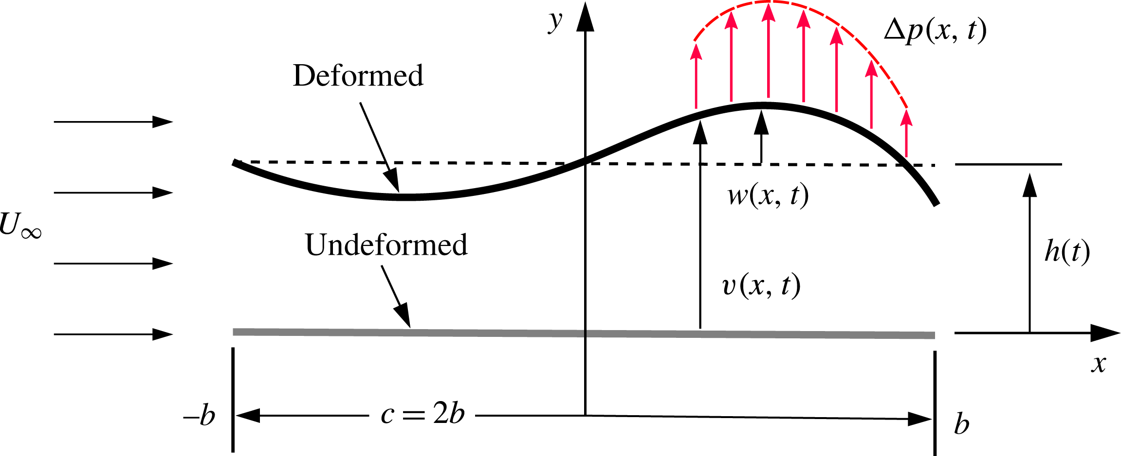
We consider a thin elastic plate with infinite span and finite chord $c$ in a two-dimensional axial free-stream flow $U_{\infty }$ , as shown in figure 1. We consider a high-Reynolds-number ( $Re$ ) flow, where the inertia forces in the surrounding fluid are important and the viscous effects are only important in the generation of circulation around the plate. To model the high- $Re$ flow, we treat the fluid as inviscid, but account for the viscous production of vorticity within boundary layers by allowing the plate to shed a flat vortex sheet from its trailing edge (Shelley & Zhang Reference Shelley and Zhang2011). We allow an imposed plunge excitation $h(t)=h_{a}\text{e}^{\text{i}2\unicode[STIX]{x03C0}ft}$ on the leading edge, where $h_{a}$ is the plunge amplitude, $f$ is the driving frequency and $t$ is the time variable. The plate deforms to an arbitrary deformation $w(x,t)$ in dynamic balance of the inertia, elastic and aerodynamic forces. This aerodynamic force is manifested as a pressure difference $\unicode[STIX]{x0394}p(x,t)$ acting on the plate. The instantaneous total displacement $v(x,t)$ of the plate can be expressed as the sum of the instantaneous plate deformation and the plunge motion, such that $v(x,t)=w(x,t)+h(t)$ . To linearize the problem, we enforce that the plate displacements are small relative to the chord, such that $|w|\ll c$ and $|h|\ll c$ .

Figure 1.

Schematic of case set-up.

2.1 Governing equation of motion

The plate with density $\unicode[STIX]{x1D70C}_{s}$ , Young’s modulus $E$ , thickness $h_{s}$ and chord $c$ is modelled as a one-dimensional Euler–Bernoulli beam, for which the governing differential equation for the transverse dynamic response is given as

(2.1)

$$\begin{eqnarray}\unicode[STIX]{x1D6F1}_{0}\frac{\unicode[STIX]{x2202}^{2}v^{\ast }}{\unicode[STIX]{x2202}t^{\ast 2}}+16\unicode[STIX]{x1D6F1}_{1}\frac{\unicode[STIX]{x2202}^{4}v^{\ast }}{\unicode[STIX]{x2202}x^{\ast 4}}=2\unicode[STIX]{x0394}p^{\ast },\end{eqnarray}$$

where $t^{\ast }=ft$ is the normalized time, $v^{\ast }=v/b$ is the normalized displacement, $x^{\ast }=x/b$ is the normalized spatial unit, $b=c/2$ is semi-chord and $\unicode[STIX]{x0394}p^{\ast }=\unicode[STIX]{x0394}p/\unicode[STIX]{x1D70C}_{f}U_{\infty }^{2}$ is the normalized pressure difference. Furthermore, $\unicode[STIX]{x1D6F1}_{0}=\unicode[STIX]{x1D70C}^{\ast }h_{s}^{\ast }(k/\unicode[STIX]{x03C0})^{2}$ is the effective inertia and $\unicode[STIX]{x1D6F1}_{1}=Eh_{s}^{\ast 3}/(12\unicode[STIX]{x1D70C}_{f}U_{\infty }^{2})$ is the effective stiffness (Kang et al. Reference Kang, Aono, Cesnik and Shyy2011), where $k=\unicode[STIX]{x03C0}fc/U_{\infty }$ is the reduced frequency, $h_{s}^{\ast }=h_{s}/c$ is the thickness ratio and $\unicode[STIX]{x1D70C}^{\ast }=\unicode[STIX]{x1D70C}_{s}/\unicode[STIX]{x1D70C}_{f}$ is the density ratio.

Using separation of variables, the plate deformation can be written as a linear summation of the products of known beam eigenfunctions in vacuo $\unicode[STIX]{x1D6F9}_{i}(x^{\ast })$ , which satisfy the boundary conditions at the leading and trailing edges, and unknown temporal solutions $\unicode[STIX]{x1D70F}_{i}(t^{\ast })$ , such that $w^{\ast }(x^{\ast },t^{\ast })=\sum _{i=1}^{\infty }\unicode[STIX]{x1D6F9}_{i}(x^{\ast })\unicode[STIX]{x1D70F}_{i}(t^{\ast })$ . Although the infinite series guarantees convergence, the number of beam eigenfunctions $N$ to be considered is determined by the physical characteristics of the problem – for example, based on the excitation frequency.

The pressure difference is expressed by a weighted linear summation of the beam eigenfunctions, such that $\unicode[STIX]{x0394}p^{\ast }(x^{\ast },t^{\ast })=\sum _{i=1}^{\infty }\unicode[STIX]{x1D6FD}_{i}(t^{\ast })\unicode[STIX]{x1D6F9}_{i}(x^{\ast })$ , where the time-dependent weighting coefficients are given by $\unicode[STIX]{x1D6FD}_{i}(t^{\ast })=1/2\int _{-1}^{1}\unicode[STIX]{x0394}p^{\ast }(x^{\ast },t^{\ast })\unicode[STIX]{x1D6F9}_{i}(x^{\ast })\,\text{d}x^{\ast }$ . We can now write (2.1) as

(2.2)

$$\begin{eqnarray}\unicode[STIX]{x1D6F1}_{0}\mathop{\sum }_{i=1}^{\infty }\unicode[STIX]{x1D6F9}_{i}\ddot{\unicode[STIX]{x1D70F}}_{i}+16\unicode[STIX]{x1D6F1}_{1}\mathop{\sum }_{i=1}^{\infty }\unicode[STIX]{x1D6F9}_{i}^{\prime \prime \prime \prime }\unicode[STIX]{x1D70F}_{i}=2\mathop{\sum }_{i=1}^{\infty }\unicode[STIX]{x1D6FD}_{i}\unicode[STIX]{x1D6F9}_{i}-\unicode[STIX]{x1D6F1}_{0}\ddot{h}^{\ast },\end{eqnarray}$$

where $h^{\ast }(t^{\ast })=h_{a}^{\ast }\text{e}^{\text{i}2\unicode[STIX]{x03C0}t^{\ast }}$ is the normalized plunge motion and $h_{a}^{\ast }=h_{a}/b$ is the normalized plunge amplitude. The operators $(\cdot )^{\prime }$ and $\dot{(\cdot )}$ indicate derivatives with respect to $x^{\ast }$ and $t^{\ast }$ , respectively. The term with $\ddot{h}^{\ast }$ is the inertia force due to the plunge excitation. Using the orthogonality of the beam eigenfunctions, such that 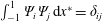$\int _{-1}^{1}\unicode[STIX]{x1D6F9}_{i}\unicode[STIX]{x1D6F9}_{j}\,\text{d}x^{\ast }=\unicode[STIX]{x1D6FF}_{ij}$ , where $\unicode[STIX]{x1D6FF}_{ij}$ is the Kronecker delta, equation (2.2) reduces to

(2.3)

$$\begin{eqnarray}\unicode[STIX]{x1D6F1}_{0}\ddot{\unicode[STIX]{x1D70F}}_{j}+\unicode[STIX]{x1D6F1}_{1}\unicode[STIX]{x1D706}_{j}^{4}\unicode[STIX]{x1D70F}_{j}=Q_{j}^{\ast }-q_{j}\unicode[STIX]{x1D6F1}_{0}\ddot{h}^{\ast },\end{eqnarray}$$

where $\unicode[STIX]{x1D706}_{j}$ are the eigenvalues associated with the beam eigenfunctions and the Fourier coefficient $q_{j}=\int _{-1}^{1}\unicode[STIX]{x1D6F9}_{j}\,\text{d}x^{\ast }/\int _{-1}^{1}\unicode[STIX]{x1D6F9}_{j}^{2}\,\text{d}x^{\ast }$ is a known constant for each beam eigenfunction. The generalized aerodynamic force is given as

(2.4)

$$\begin{eqnarray}Q_{j}^{\ast }(t^{\ast })=\int _{-1}^{1}\unicode[STIX]{x0394}p^{\ast }(x^{\ast },t^{\ast })\unicode[STIX]{x1D6F9}_{j}(x^{\ast })\,\text{d}x^{\ast }.\end{eqnarray}$$

2.2 Aerodynamic model

We further assume the fluid to be irrotational and incompressible, such that the potential flow equations govern the flow, for which a velocity potential $\unicode[STIX]{x1D6F7}$ exists and satisfies the Laplace equation, $\unicode[STIX]{x1D6FB}^{2}\unicode[STIX]{x1D6F7}=0$ . We enforce the slip boundary condition, such that the normal velocity of the fluid at the surface of the plate goes to zero, i.e. $(\unicode[STIX]{x1D735}\unicode[STIX]{x1D6F7}-\boldsymbol{v}_{rel})\boldsymbol{\cdot }\boldsymbol{n}=0,$ where $\boldsymbol{v}_{rel}=(0,\unicode[STIX]{x2202}v/\unicode[STIX]{x2202}t)$ . Since the solution to Laplace’s equation is linear, its solution can be written as $\unicode[STIX]{x1D6F7}=\unicode[STIX]{x1D719}+\unicode[STIX]{x1D719}_{\infty }$ , where $\unicode[STIX]{x1D719}$ is the perturbation velocity potential and $\unicode[STIX]{x1D719}_{\infty }=U_{\infty }x$ is the velocity potential due to the free stream. The surface normal is defined as $\boldsymbol{n}=1/|\unicode[STIX]{x1D735}v|(-\unicode[STIX]{x2202}v/\unicode[STIX]{x2202}x,1)$ , where $\unicode[STIX]{x2202}v/\unicode[STIX]{x2202}x$ is the local slope of the plate surface. Then, the vertical perturbation velocity at the surface of the plate becomes

(2.5)

$$\begin{eqnarray}\frac{\unicode[STIX]{x2202}\unicode[STIX]{x1D719}}{\unicode[STIX]{x2202}y}=U_{\infty }\frac{\unicode[STIX]{x2202}v}{\unicode[STIX]{x2202}x}+\frac{\unicode[STIX]{x2202}v}{\unicode[STIX]{x2202}t}+\frac{\unicode[STIX]{x2202}\unicode[STIX]{x1D719}}{\unicode[STIX]{x2202}x}\frac{\unicode[STIX]{x2202}v}{\unicode[STIX]{x2202}x}.\end{eqnarray}$$

In addition, the solution must satisfy Kelvin’s theorem, such that the change in circulation inside the control volume must remain zero. We enforce that far downstream the effects of any perturbation must vanish. Finally, we must satisfy the Kutta condition, which states that no infinite velocities may exist at the trailing edge of the plate, i.e. $|\unicode[STIX]{x1D735}(\unicode[STIX]{x1D719}(x_{TE}^{\ast },t))|<\infty$ , where $x_{TE}^{\ast }=1$ . Following the approach of Theodorsen (Reference Theodorsen1935), the perturbation velocity potential is divided into two parts: the non-circulatory velocity potential $\unicode[STIX]{x1D719}_{nc}$ and the circulatory velocity potential $\unicode[STIX]{x1D719}_{c}$ , such that $\unicode[STIX]{x1D719}=\unicode[STIX]{x1D719}_{nc}+\unicode[STIX]{x1D719}_{c}$ .

2.2.1 Non-circulatory flow

The non-circulatory flow is modelled using a source/sink sheet, which is composed of continuous source/sink pairs of strength $\pm \unicode[STIX]{x0394}\unicode[STIX]{x1D70E}$ along the $x$ -axis under the small plate displacement assumption, spanning from the leading edge to the trailing edge. The velocity potential for the source/sink sheet is given by (Theodorsen Reference Theodorsen1935)

(2.6)

$$\begin{eqnarray}\unicode[STIX]{x1D719}_{nc}=\frac{b}{4\unicode[STIX]{x03C0}}\int _{-1}^{1}\unicode[STIX]{x1D70E}(x_{1}^{\ast },t^{\ast })\log \frac{(x^{\ast }-x_{1}^{\ast })^{2}+(\sqrt{1-x^{\ast 2}}-\sqrt{1-x_{1}^{\ast 2}})^{2}}{(x^{\ast }-x_{1}^{\ast })^{2}+(\sqrt{1-x^{\ast 2}}+\sqrt{1-x_{1}^{\ast 2}})^{2}}\,\text{d}x_{1}^{\ast },\end{eqnarray}$$

where $x_{1}$ is the location of the source/sink. The influence from the curvature of the flexible plate is realized by a spatially varying source/sink sheet strength $\unicode[STIX]{x1D70E}(x_{1}^{\ast },t^{\ast })$ , which is a known function derived from satisfying the slip boundary condition, given as

(2.7)

$$\begin{eqnarray}\unicode[STIX]{x1D70E}(x_{1}^{\ast },t^{\ast })=2\left(U_{\infty }\frac{\unicode[STIX]{x2202}v^{\ast }}{\unicode[STIX]{x2202}x_{1}^{\ast }}+bf\frac{\unicode[STIX]{x2202}v^{\ast }}{\unicode[STIX]{x2202}t^{\ast }}\right),\end{eqnarray}$$

where we have neglected higher-order terms. The pressure difference due to the non-circulatory flow follows from the unsteady Bernoulli equation as

(2.8)

$$\begin{eqnarray}\unicode[STIX]{x0394}p_{nc}(x^{\ast },t^{\ast })=2\unicode[STIX]{x1D70C}_{f}\left(\frac{U_{\infty }}{b}\frac{\unicode[STIX]{x2202}\unicode[STIX]{x1D719}_{nc}}{\unicode[STIX]{x2202}x^{\ast }}+f\frac{\unicode[STIX]{x2202}\unicode[STIX]{x1D719}_{nc}}{\unicode[STIX]{x2202}t^{\ast }}\right),\end{eqnarray}$$

where we again have neglected higher-order terms.

2.2.2 Circulatory flow

The circulatory flow is modelled using a vortex sheet, which is composed of continuous vortex pairs of strength $\unicode[STIX]{x0394}\unicode[STIX]{x1D6E4}$ along the $x$ -axis under the small plate displacement assumption, spanning from the trailing edge to infinity. This vortex sheet satisfies Kelvin’s theorem and does not disrupt the slip boundary condition. We can express the strength of the circulation shed into the wake along the $x$ -axis as $\unicode[STIX]{x0394}\unicode[STIX]{x1D6E4}=b\unicode[STIX]{x1D6FE}_{w}(x^{\ast },t^{\ast })\,\text{d}x_{0}^{\ast }$ , where $\unicode[STIX]{x1D6FE}_{w}$ is the circulation per unit length and where $x_{0}$ is the location of the point vortex. The velocity potential for the vortex sheet is given as (Theodorsen Reference Theodorsen1935)

(2.9)

$$\begin{eqnarray}\unicode[STIX]{x1D719}_{c}(x^{\ast },t^{\ast })=-\frac{b}{2\unicode[STIX]{x03C0}}\int _{1}^{\infty }\tan ^{-1}\frac{\sqrt{1-x^{\ast 2}}\sqrt{x_{0}^{\ast 2}-1}}{1-x^{\ast }x_{0}^{\ast }}\unicode[STIX]{x1D6FE}_{w}(x_{0}^{\ast },t^{\ast })\,\text{d}x_{0}^{\ast }.\end{eqnarray}$$

Enforcing the Kutta condition, we ensure that the flow velocity magnitude at the trailing edge $x^{\ast }=1$ is to be finite, such that $\unicode[STIX]{x2202}[\unicode[STIX]{x1D719}_{nc}(1,t^{\ast })+\unicode[STIX]{x1D719}_{c}(1,t^{\ast })]/\unicode[STIX]{x2202}x^{\ast }=\unicode[STIX]{x1D709}$ , where $\unicode[STIX]{x1D709}$ is a finite constant. The Kutta condition dictates the amount of vorticity shed into the wake, leading to the following relation

(2.10)

$$\begin{eqnarray}\frac{1}{2\unicode[STIX]{x03C0}}\int _{1}^{\infty }\sqrt{\frac{x_{0}^{\ast }+1}{x_{0}^{\ast }-1}}\unicode[STIX]{x1D6FE}_{w}(x_{0}^{\ast },t^{\ast })\,\text{d}x_{0}^{\ast }=\left[-\frac{\sqrt{1-x^{\ast 2}}}{b}\frac{\unicode[STIX]{x2202}\unicode[STIX]{x1D719}_{nc}}{\unicode[STIX]{x2202}x^{\ast }}\right]_{x^{\ast }=1}.\end{eqnarray}$$

We assume that the wake vortex sheet strength is harmonic and can be written in terms of $k$ as $\unicode[STIX]{x1D6FE}_{w}(x^{\ast },t^{\ast })=\bar{\unicode[STIX]{x1D6FE}}_{w}\text{e}^{\text{i}(2\unicode[STIX]{x03C0}t^{\ast }-kx^{\ast })}$ , where $\bar{\unicode[STIX]{x1D6FE}}_{w}$ is the magnitude. From the unsteady Bernoulli equation and with some manipulation, the pressure due to the circulatory flow can be expressed as

(2.11)

$$\begin{eqnarray}\unicode[STIX]{x0394}p_{c}(x^{\ast },t^{\ast })=2\unicode[STIX]{x1D70C}_{f}U_{\infty }K(t^{\ast })\frac{C(k)+x^{\ast }(1-C(k))}{\sqrt{1-x^{\ast 2}}},\end{eqnarray}$$

where $C(k)$ is Theodorsen’s function (Theodorsen Reference Theodorsen1935), defined as

(2.12)

$$\begin{eqnarray}C(k)=\frac{\displaystyle \int _{1}^{\infty }\frac{x_{0}^{\ast }}{\sqrt{x_{0}^{\ast 2}-1}}\text{e}^{-\text{i}kx_{0}^{\ast }}\,\text{d}x_{0}^{\ast }}{\displaystyle \int _{1}^{\infty }\frac{\sqrt{x_{0}^{\ast }+1}}{\sqrt{x_{0}^{\ast }-1}}\text{e}^{-\text{i}kx_{0}^{\ast }}\,\text{d}x_{0}^{\ast }}=\frac{H_{1}^{(2)}(k)}{H_{1}^{(2)}(k)+\text{i}H_{0}^{(2)}(k)},\end{eqnarray}$$

where $H_{n}^{(2)}$ are the $n\text{th}$ -order Hankel functions of the second kind, and is a function of reduced frequency only. The time-dependent function $K(t^{\ast })$ is related to the amount of vorticity shed at the trailing edge, defined as

(2.13)

$$\begin{eqnarray}K(t^{\ast })=\frac{1}{2\unicode[STIX]{x03C0}}\int _{1}^{\infty }\sqrt{\frac{x_{0}^{\ast }+1}{x_{0}^{\ast }-1}}\unicode[STIX]{x1D6FE}_{w}(x_{0}^{\ast },t^{\ast })\,\text{d}x_{0}^{\ast },\end{eqnarray}$$

which is also given in (2.10). To obtain the complete pressure difference we sum the pressures due to non-circulatory and circulatory flows, such that $\unicode[STIX]{x0394}p=\unicode[STIX]{x0394}p_{nc}+\unicode[STIX]{x0394}p_{c}$ .

3 Solution

3.1 Chebyshev polynomial expansion

The plate deformation depends on the generalized aerodynamic force $Q^{\ast }$ given in (2.4). At the same time, $Q^{\ast }$ depends on $\unicode[STIX]{x0394}p^{\ast }$ , which in turn, depends on the plate deformation. To analytically solve this two-way coupled problem, we express the plate deformation in a Chebyshev polynomial expansion of the first kind as

(3.1)

$$\begin{eqnarray}w^{\ast }(x^{\ast },t^{\ast })=\mathop{\sum }_{i=1}^{\infty }\unicode[STIX]{x1D6F9}_{i}(x^{\ast })\unicode[STIX]{x1D70F}_{i}(t^{\ast })=\mathop{\sum }_{i=1}^{\infty }\unicode[STIX]{x1D70F}_{i}(t^{\ast })\mathop{\sum }_{n=0}^{\infty }c_{n,i}T_{n}(x^{\ast }),\end{eqnarray}$$

where the Chebyshev polynomials $T_{n}(x^{\ast })$ are a series of orthogonal polynomials within the interval $-1\leqslant x^{\ast }\leqslant 1$ and with a weight of $1/\sqrt{1-x^{\ast 2}}$ , defined by the recurrence relation

(3.2)

$$\begin{eqnarray}T_{n}(x^{\ast })=\left\{\begin{array}{@{}ll@{}}1\quad & n=0\\ x^{\ast }\quad & n=1\\ 2x^{\ast }T_{n}(x^{\ast })-T_{n-1}(x^{\ast })\quad & n\geqslant 2.\end{array}\right.\end{eqnarray}$$

This allows the exact evaluation of the non-circulatory velocity potential (Walker & Patil Reference Walker and Patil2014), given in (2.6). The Chebyshev polynomials have not only been used for two-dimensional incompressible flow aerodynamic models, but also for three-dimensional subsonic compressible aerodynamic models (Watkins, Woolston & Cunningham Reference Watkins, Woolston and Cunningham1959; Landahl & Stark Reference Landahl and Stark1968), which is also called the kernel function method. The Chebyshev coefficients $c_{n,i}$ are constants, referring to the $i\text{th}$ beam eigenfunction and are determined by

(3.3)

$$\begin{eqnarray}c_{n,i}=\left\{\begin{array}{@{}ll@{}}\displaystyle \frac{1}{\unicode[STIX]{x03C0}}\int _{-1}^{1}\frac{1}{\sqrt{1-x^{\ast 2}}}\unicode[STIX]{x1D6F9}_{i}(x^{\ast })T_{0}(x^{\ast })\,\text{d}x^{\ast }\quad & n=0\\ \displaystyle \frac{2}{\unicode[STIX]{x03C0}}\int _{-1}^{1}\frac{1}{\sqrt{1-x^{\ast 2}}}\unicode[STIX]{x1D6F9}_{i}(x^{\ast })T_{n}(x^{\ast })\,\text{d}x^{\ast }\quad & n\geqslant 1.\end{array}\right.\end{eqnarray}$$

The Chebychev expansion of each beam mode rapidly converges because the beam eigenfunctions are smooth functions. Therefore, the Chebyshev infinite series does not need to be considered and a sufficiently large number ( $M$ ) of terms can be used.

3.2 Generalized aerodynamic force

By expressing the plate deformation in a Chebyshev expansion, the source/sink sheet strength given in (2.7) can be expressed as a polynomial containing the Chebyshev coefficients, which include the influence from the plate curvature. The non-circulatory velocity potential given in (2.6), as well as $\unicode[STIX]{x0394}p^{\ast }$ given by (2.11) and (2.8), can be integrated exactly (see online supplementary material available at https://doi.org/10.1017/jfm.2018.264). Note that the Cauchy principal value should be taken (Katz & Plotkin Reference Katz and Plotkin2001). Then, the generalized aerodynamic force given in (2.4) can be evaluated exactly, by once again expressing $\unicode[STIX]{x1D6F9}_{j}$ in a Chebyshev expansion, yielding

(3.4)

$$\begin{eqnarray}Q_{j}^{\ast }(t^{\ast })=\int _{-1}^{1}\unicode[STIX]{x0394}p^{\ast }\unicode[STIX]{x1D6F9}_{j}\,\text{d}x^{\ast }=-\mathop{\sum }_{i=1}^{\infty }[\unicode[STIX]{x1D705}_{ji}^{m}\ddot{\unicode[STIX]{x1D70F}}_{i}+\unicode[STIX]{x1D705}_{ji}^{c}\dot{\unicode[STIX]{x1D70F}}_{i}+\unicode[STIX]{x1D705}_{ji}^{k}\unicode[STIX]{x1D70F}_{i}]-\unicode[STIX]{x1D707}_{j}\ddot{h}^{\ast }-\unicode[STIX]{x1D702}_{j}{\dot{h}}^{\ast },\end{eqnarray}$$

where

(3.5)

$$\begin{eqnarray}\displaystyle & \displaystyle \unicode[STIX]{x1D705}_{ji}^{m}=\frac{k^{2}}{4\unicode[STIX]{x03C0}}\left(c_{0,i}c_{0,j}+\frac{1}{8}c_{1,i}c_{1,j}-\frac{1}{2}(c_{0,i}c_{2,j}+c_{2,i}c_{0,j})+\unicode[STIX]{x1D6F4}_{ji}^{6}-\unicode[STIX]{x1D6F4}_{ji}^{7}\right), & \displaystyle\end{eqnarray}$$

(3.6)

$$\begin{eqnarray}\displaystyle & \displaystyle \unicode[STIX]{x1D705}_{ji}^{c}=\frac{k}{4}(C(k)(2c_{0,i}+c_{1,i})(2c_{0,j}-c_{1,j})+c_{1,i}(2c_{0,j}+c_{1,j})+2\unicode[STIX]{x1D6F4}_{ji}^{8}), & \displaystyle\end{eqnarray}$$

(3.7)

$$\begin{eqnarray}\displaystyle & \displaystyle \unicode[STIX]{x1D705}_{ji}^{k}=\unicode[STIX]{x03C0}(C(k)(2c_{0,j}-c_{1,j})\unicode[STIX]{x1D6F4}_{i}^{1}+c_{1,j}\unicode[STIX]{x1D6F4}_{i}^{1}-\unicode[STIX]{x1D6F4}_{ji}^{5}), & \displaystyle\end{eqnarray}$$

(3.8a,b )

$$\begin{eqnarray}\displaystyle \unicode[STIX]{x1D707}_{j}=\frac{k^{2}}{8\unicode[STIX]{x03C0}}(2c_{0,j}-c_{2,j}),\quad \unicode[STIX]{x1D702}_{j}=\frac{k}{2}C(k)(2c_{0,j}-c_{1,j}), & & \displaystyle\end{eqnarray}$$

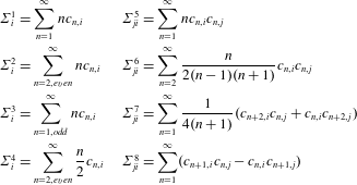
where the $\unicode[STIX]{x1D6F4}$ symbols are summations of Chebyshev coefficients given in table 1 for the $i\text{th}$ beam eigenfunction. The $\unicode[STIX]{x1D705}$ terms are related to the plate dynamics, where $\unicode[STIX]{x1D705}^{m}$ is the aeroelastic mass, $\unicode[STIX]{x1D705}^{c}$ is the aeroelastic damping and $\unicode[STIX]{x1D705}^{k}$ is the aeroelastic stiffness. The terms $\unicode[STIX]{x1D707}$ and $\unicode[STIX]{x1D702}$ are related to the imposed plunge excitation, where $\unicode[STIX]{x1D707}$ is the aerodynamic inertia and $\unicode[STIX]{x1D702}$ is the aerodynamic damping. Note that $Q^{\ast }$ is non-local due to $\unicode[STIX]{x0394}p^{\ast }$ being expressed by one set of beam eigenfunctions and then multiplied by another set of beam eigenfunctions.

Table 1.

Chebyshev coefficient summations for the $i\text{th}$ beam eigenfunction.

3.3 Solution to the equation of motion

By moving the terms related to $\unicode[STIX]{x1D70F}$ to the left-hand side and leaving the forcing terms on the right-hand side, we can write (2.3) as

(3.9)

$$\begin{eqnarray}\unicode[STIX]{x1D648}\ddot{\unicode[STIX]{x1D749}}+\unicode[STIX]{x1D63E}\dot{\unicode[STIX]{x1D749}}+\unicode[STIX]{x1D646}\unicode[STIX]{x1D749}=\boldsymbol{F},\end{eqnarray}$$

where the elements of each matrix are as follows: the mass matrix $\unicode[STIX]{x1D614}_{ji}=\unicode[STIX]{x1D6F1}_{0}\unicode[STIX]{x1D6FF}_{ji}+\unicode[STIX]{x1D705}_{ji}^{m}$ , the damping matrix $\unicode[STIX]{x1D60A}_{ji}=\unicode[STIX]{x1D705}_{ji}^{c}$ , the stiffness matrix $\unicode[STIX]{x1D612}_{ji}=\unicode[STIX]{x1D6F1}_{1}\unicode[STIX]{x1D706}_{j}^{4}\unicode[STIX]{x1D6FF}_{ji}+\unicode[STIX]{x1D705}_{ji}^{k}$ and the force vector $F_{j}=-(q_{j}\unicode[STIX]{x1D6F1}_{0}+\unicode[STIX]{x1D707}_{j})\ddot{h^{\ast }}-\unicode[STIX]{x1D702}_{j}\dot{h^{\ast }}$ . Due to the non-local behaviour of $Q^{\ast }$ , the mass, damping and stiffness matrices are fully populated with known coefficients. Therefore, we have an infinite number of non-local second-order linear ordinary differential equations.

3.3.1 Homogeneous solution

We assume harmonic motion in the form $\unicode[STIX]{x1D749}=\bar{\unicode[STIX]{x1D749}}\text{e}^{st}$ , where $\bar{\unicode[STIX]{x1D749}}$ is the modal amplitude and $s=\unicode[STIX]{x1D701}+\text{i}k$ is the Laplace variable, where $\unicode[STIX]{x1D701}$ is the modal damping. Substituting into (3.9) and setting the force vector to zero yields,

(3.10)

$$\begin{eqnarray}[s^{2}\unicode[STIX]{x1D648}(s)+s\unicode[STIX]{x1D63E}(s)+\unicode[STIX]{x1D646}(s)]\bar{\unicode[STIX]{x1D749}}=\mathbf{0}.\end{eqnarray}$$

In order for the system to have a non-trivial solution, we solve the eigenvalue problem given as

(3.11)

$$\begin{eqnarray}|s\unicode[STIX]{x1D644}-\unicode[STIX]{x1D63C}(s)|=0,\end{eqnarray}$$

where we have transformed the system into state-space form with $\unicode[STIX]{x1D644}$ being the identity matrix and $\unicode[STIX]{x1D63C}$ the system state matrix, given as

(3.12)

$$\begin{eqnarray}\unicode[STIX]{x1D63C}=\left[\begin{array}{@{}cc@{}}\mathbf{0} & \unicode[STIX]{x1D644}\\ -\unicode[STIX]{x1D648}^{-1}\unicode[STIX]{x1D646} & -\unicode[STIX]{x1D648}^{-1}\unicode[STIX]{x1D63E}\end{array}\right],\end{eqnarray}$$

which can be solved iteratively.

3.3.2 Inhomogeneous solution

Because we consider a harmonic forcing function $h$ in our study and (3.9) is a system of second-order linear ordinary differential equations, we try a trial solution of the form $\unicode[STIX]{x1D70F}_{j}=Z_{j}\text{e}^{\text{i}\unicode[STIX]{x1D711}_{j}}\text{e}^{\text{i}2\unicode[STIX]{x03C0}t^{\ast }}$ , where $Z_{j}$ is the amplitude and $\unicode[STIX]{x1D711}_{j}$ is the phase lag. Inserting into (3.9) yields

(3.13)

$$\begin{eqnarray}\mathop{\sum }_{i=1}^{\infty }[-4\unicode[STIX]{x03C0}^{2}(\unicode[STIX]{x1D6F1}_{0}\unicode[STIX]{x1D6FF}_{ji}+\unicode[STIX]{x1D705}_{ji}^{m})+\text{i}2\unicode[STIX]{x03C0}\unicode[STIX]{x1D705}_{ji}^{c}+\unicode[STIX]{x1D6F1}_{1}\unicode[STIX]{x1D706}_{j}^{4}\unicode[STIX]{x1D6FF}_{ji}+\unicode[STIX]{x1D705}_{ji}^{k}]Z_{i}\text{e}^{\text{i}\unicode[STIX]{x1D711}_{i}}=4\unicode[STIX]{x03C0}^{2}h_{a}^{\ast }(q_{j}\unicode[STIX]{x1D6F1}_{0}+\unicode[STIX]{x1D707}_{j})-\text{i}2\unicode[STIX]{x03C0}h_{a}^{\ast }\unicode[STIX]{x1D702}_{j}.\end{eqnarray}$$

Equation (3.13) represents the $j\text{th}$ equation, which can be solved analytically for $Z_{i}\text{e}^{\text{i}\unicode[STIX]{x1D711}_{i}}$ . The solution to the plate deformation is given as $w^{\ast }(x^{\ast },t^{\ast })=\sum _{j=1}^{\infty }\unicode[STIX]{x1D6F9}_{j}(x^{\ast })Z_{j}\text{e}^{\text{i}\unicode[STIX]{x1D711}_{j}}\text{e}^{\text{i}2\unicode[STIX]{x03C0}t^{\ast }}$ .

3.4 Aerodynamic performance

3.4.1 Lift

The generated lift can be obtained by integrating the pressure over the plate chord, such that $L^{\prime }(t^{\ast })=b\int _{-1}^{1}\unicode[STIX]{x0394}p(x^{\ast },t^{\ast })\,\text{d}x^{\ast }$ . The exact expression for the generated lift for the $i\text{th}$ beam mode is given as

(3.14)

$$\begin{eqnarray}\displaystyle L_{i}^{\prime }(t^{\ast }) & = & \displaystyle \text{Re}\left[-\unicode[STIX]{x03C0}\unicode[STIX]{x1D70C}_{f}b^{2}\left(bf^{2}\ddot{h}^{\ast }+{\textstyle \frac{1}{2}}b(2c_{0,i}-c_{2,i})f^{2}\ddot{\unicode[STIX]{x1D70F}}_{i}+U_{\infty }c_{1,i}f\,\dot{\unicode[STIX]{x1D70F}}_{i}\right)\right.\nonumber\\ \displaystyle & & \displaystyle \left.-\,2\unicode[STIX]{x03C0}\unicode[STIX]{x1D70C}_{f}U_{\infty }bC(k)\left(bf{\dot{h}}^{\ast }+{\textstyle \frac{1}{2}}b(2c_{0,i}+c_{1,i})f\dot{\unicode[STIX]{x1D70F}}_{i}+U_{\infty }\unicode[STIX]{x1D6F4}_{i}^{1}\unicode[STIX]{x1D70F}_{i}\right)\right],\end{eqnarray}$$

where we have taken the real part of the complex-valued solution. The first term is from the non-circulatory flow and the second term is from the circulatory flow. The total lift is the summation of all the $i\text{th}$ terms, such that $L^{\prime }(t^{\ast })=\sum _{i=1}^{\infty }L_{i}^{\prime }(t^{\ast })$ .

3.4.2 Thrust

The generated thrust force $T^{\prime }$ is composed of two components, the thrust due to the pressure difference $T_{p}^{\prime }$ and the thrust do to the leading-edge suction $T_{LES}^{\prime }$ . The thrust due to the pressure is obtained by integrating $\unicode[STIX]{x0394}p$ multiplied by the local slope of the plate over the chord, such that $T_{p}^{\prime }(t^{\ast })=b\int _{-1}^{1}\unicode[STIX]{x0394}p(x^{\ast },t^{\ast })(\unicode[STIX]{x2202}v^{\ast }/\unicode[STIX]{x2202}x^{\ast })\,\text{d}x^{\ast }$ . The exact expression for $T_{p}$ for the $i\text{th}$ beam mode is given as

(3.15)

$$\begin{eqnarray}\displaystyle T_{p,i}^{\prime }(t^{\ast }) & = & \displaystyle \text{Re}[\!-\unicode[STIX]{x03C0}\unicode[STIX]{x1D70C}_{f}b[2U_{\infty }^{2}(4\unicode[STIX]{x1D6F4}_{i}^{4}\unicode[STIX]{x1D6F4}_{i}^{4}+C(k)(\unicode[STIX]{x1D6F4}_{i}^{3}-\unicode[STIX]{x1D6F4}_{i}^{2})\unicode[STIX]{x1D6F4}_{i}^{1})\unicode[STIX]{x1D70F}_{i}^{2}\nonumber\\ \displaystyle & & \displaystyle +\,2U_{\infty }bC(k)(\unicode[STIX]{x1D6F4}_{i}^{3}-\unicode[STIX]{x1D6F4}_{i}^{2})f\unicode[STIX]{x1D70F}_{i}{\dot{h}}^{\ast }\nonumber\\ \displaystyle & & \displaystyle +\,U_{\infty }b(2\unicode[STIX]{x1D6F4}_{ii}^{5}+(C(k)(2c_{0,i}+c_{1,i})-c_{1,i})(\unicode[STIX]{x1D6F4}_{i}^{3}-\unicode[STIX]{x1D6F4}_{i}^{2}))f\unicode[STIX]{x1D70F}_{i}\dot{\unicode[STIX]{x1D70F}}_{i}\nonumber\\ \displaystyle & & \displaystyle +\,b^{2}c_{0,i}c_{1,i}\,f^{2}\unicode[STIX]{x1D70F}_{i}\ddot{\unicode[STIX]{x1D70F}}_{i}+b^{2}c_{1,i}\,f^{2}\unicode[STIX]{x1D70F}_{i}\ddot{h}^{\ast }]],\end{eqnarray}$$

where we have taken the real part of the complex-valued solution.

The thrust due to the leading-edge suction is given as $T_{LES}=\unicode[STIX]{x03C0}\unicode[STIX]{x1D70C}_{f}S^{2}$ (von Karman & Burgers Reference von Karman, Burgers and Durand1935). The leading-edge suction $S$ is generated by the vorticity at the leading edge and was determined by von Karman & Burgers (Reference von Karman, Burgers and Durand1935). The exact expression for the thrust due to the leading-edge suction for the $i\text{th}$ beam mode is given as

(3.16)

$$\begin{eqnarray}\displaystyle T_{LES,i}^{\prime }(t^{\ast }) & = & \displaystyle \text{Re}\left[\unicode[STIX]{x03C0}\unicode[STIX]{x1D70C}_{f}b\left[2U_{\infty }^{2}(C(k)\unicode[STIX]{x1D6F4}_{i}^{1}-2\unicode[STIX]{x1D6F4}_{i}^{4})^{2}\unicode[STIX]{x1D70F}_{i}^{2}\right.\right.\nonumber\\ \displaystyle & & \displaystyle +\,2b^{2}C(k)(C(k)(2c_{0,i}+c_{1,i})-c_{1,i})f^{2}\dot{\unicode[STIX]{x1D70F}}_{i}{\dot{h}}^{\ast }\nonumber\\ \displaystyle & & \displaystyle +\,{\textstyle \frac{1}{2}}b^{2}(c_{1,i}-C(k)(2c_{0,i}+c_{1,i}))^{2}f^{2}\dot{\unicode[STIX]{x1D70F}}_{i}^{2}+4U_{\infty }bC(k)(C(k)\unicode[STIX]{x1D6F4}_{i}^{1}-2\unicode[STIX]{x1D6F4}_{i}^{4})f\unicode[STIX]{x1D70F}_{i}{\dot{h}}^{\ast }\nonumber\\ \displaystyle & & \displaystyle +\left.\left.2U_{\infty }b(C(k)(2c_{0,i}+c_{1,i})-c_{1,i})(C(k)\unicode[STIX]{x1D6F4}_{i}^{1}-2\unicode[STIX]{x1D6F4}_{i}^{4})f\unicode[STIX]{x1D70F}_{i}\dot{\unicode[STIX]{x1D70F}}_{i}+2b^{2}C(k)^{2}f^{2}{\dot{h}}^{\ast 2}\right]\right],\nonumber\\ \displaystyle & & \displaystyle\end{eqnarray}$$

where again we have taken the real part of the complex-valued solution. The total generated thrust is the summation of all the $i\text{th}$ terms, such that $T^{\prime }(t^{\ast })=\sum _{i=1}^{\infty }[T_{p,i}^{\prime }(t^{\ast })+T_{LES,i}^{\prime }(t^{\ast })]$ .

3.4.3 Power

To drive the motion, power is required and is equal to time rate of work done on the fluid. Therefore, the power is equal to $\unicode[STIX]{x0394}p$ multiplied by the plate velocity and integrated over the chord, such that $P^{\prime }(t^{\ast })=bf\int _{-1}^{1}\unicode[STIX]{x0394}p(x^{\ast },t^{\ast })(\unicode[STIX]{x2202}v^{\ast }/\unicode[STIX]{x2202}t^{\ast })\,\text{d}x^{\ast }$ , which includes the effects of the plate deformation. The exact expression for the required input power for the $i\text{th}$ beam mode is given as

(3.17)

$$\begin{eqnarray}\displaystyle P_{i}^{\prime }(t^{\ast }) & = & \displaystyle \text{Re}\left[-\unicode[STIX]{x03C0}\unicode[STIX]{x1D70C}_{f}b^{2}\left[U_{\infty }^{2}(c_{1,i}\unicode[STIX]{x1D6F4}_{i}^{1}-\unicode[STIX]{x1D6F4}_{ii}^{5}+C(k)(2c_{0,i}-c_{1,i})\unicode[STIX]{x1D6F4}_{i}^{1})f\unicode[STIX]{x1D70F}_{i}\dot{\unicode[STIX]{x1D70F}}_{i}\right.\right.\nonumber\\ \displaystyle & & \displaystyle +\,2U_{\infty }^{2}C(k)\unicode[STIX]{x1D6F4}_{i}^{1}f\unicode[STIX]{x1D70F}_{i}{\dot{h}}^{\ast }\nonumber\\ \displaystyle & & \displaystyle +\,{\textstyle \frac{1}{2}}U_{\infty }b(2c_{0,i}+c_{1,i})(C(k)(2c_{0,i}-c_{1,i})+c_{1,i})f^{2}\dot{\unicode[STIX]{x1D70F}}_{i}^{2}+2U_{\infty }bC(k)f^{2}{\dot{h}}^{\ast 2}\nonumber\\ \displaystyle & & \displaystyle +\,U_{\infty }b(4C(k)c_{0,i}+c_{1,i})f^{2}\dot{\unicode[STIX]{x1D70F}}_{i}{\dot{h}}^{\ast }+b^{2}(c_{0,i}^{2}+{\textstyle \frac{1}{8}}c_{1,i}^{2}-c_{0,i}c_{2,i}+\unicode[STIX]{x1D6F4}_{ii}^{6}-\unicode[STIX]{x1D6F4}_{ii}^{7})f^{3}\dot{\unicode[STIX]{x1D70F}}_{i}\ddot{\unicode[STIX]{x1D70F}}_{i}\nonumber\\ \displaystyle & & \displaystyle +\left.\left.{\textstyle \frac{1}{2}}b^{2}(2c_{0,i}-c_{2,i})f^{3}(\dot{\unicode[STIX]{x1D70F}}_{i}\ddot{h}^{\ast }+\ddot{\unicode[STIX]{x1D70F}}_{i}{\dot{h}}^{\ast })+b^{2}f^{3}{\dot{h}}^{\ast }\ddot{h}^{\ast }\right]\right],\end{eqnarray}$$

where once again we have taken the real part of the complex-valued solution. The total power is the summation of all $i\text{th}$ terms, such that $P^{\prime }(t^{\ast })=\sum _{i=1}^{\infty }P_{i}^{\prime }(t^{\ast })$ .

4 Comparisons to results in the literature

Although the current model does not enforce any restrictions on the boundary conditions, we consider the cantilever beam configuration to compare to the results from the literature. The cantilever beam is described by no displacement or rotation at the leading edge and no bending or shear at the trailing edge. The beam eigenfunctions for the cantilever beam are given by (Timoshenko Reference Timoshenko2017)

(4.1)

$$\begin{eqnarray}\displaystyle \unicode[STIX]{x1D6F9}_{i}(x^{\ast }) & = & \displaystyle \cosh \left(\frac{\unicode[STIX]{x1D706}_{i}}{2}(x^{\ast }+1)\right)-\cos \left(\frac{\unicode[STIX]{x1D706}_{i}}{2}(x^{\ast }+1)\right)\nonumber\\ \displaystyle & & \displaystyle -\,\frac{\cosh (\unicode[STIX]{x1D706}_{i})+\cos (\unicode[STIX]{x1D706}_{i})}{\sinh (\unicode[STIX]{x1D706}_{i})+\sin (\unicode[STIX]{x1D706}_{i})}\left[\sinh \left(\frac{\unicode[STIX]{x1D706}_{i}}{2}(x^{\ast }+1)\right)-\sin \left(\frac{\unicode[STIX]{x1D706}_{i}}{2}(x^{\ast }+1)\right)\right],\end{eqnarray}$$

where $\unicode[STIX]{x1D706}_{i}$ is obtained through the transcendental equation $\cos (\unicode[STIX]{x1D706}_{i})\cosh (\unicode[STIX]{x1D706}_{i})+1=0$ .

4.1 Stability boundary comparison

The homogeneous solution given in § 3.3.1 provides information about the natural state of the system. In aeroelastic systems, there exists a minimum flow speed and corresponding frequency at which a given structure submerged in a fluid with a given density will exhibit sustained harmonic oscillations (Bisplinghoff, Ashley & Halfman Reference Bisplinghoff, Ashley and Halfman1996). This minimum flow speed is called the flutter speed and the frequency of the oscillation the flutter frequency $f_{f}$ .

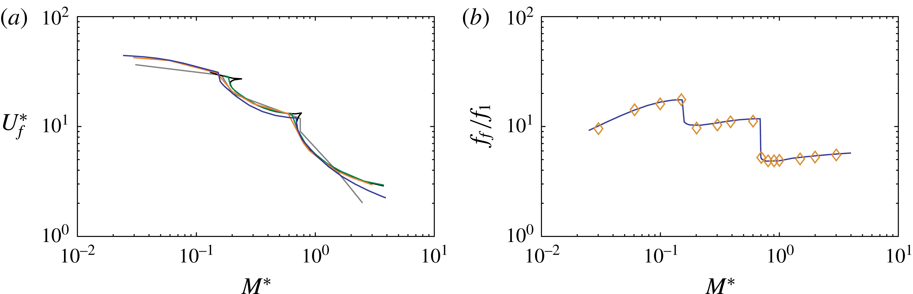
The non-dimensional flutter speed $U_{f}^{\ast }=\unicode[STIX]{x1D6F1}_{1}^{-1/2}$ , where $\unicode[STIX]{x1D6F1}_{1}$ is calculated with the flutter speed, and flutter frequency ratio $f_{f}/f_{1}$ , where $f_{1}$ is the first natural frequency of the beam, are shown in figure 2 as a function of the mass ratio $M^{\ast }=\unicode[STIX]{x1D70C}^{\ast }h_{s}^{\ast }$ . The jumps indicate mode switching, where the flutter mode shape and frequency instantaneously change to another mode shape and corresponding frequency.

There is good agreement on the flutter boundary between the current result and the results by Kornecki et al. (Reference Kornecki, Dowell and O’Brien1976), Guo & Païdoussis (Reference Guo and Païdoussis2000), Watanabe et al. (Reference Watanabe, Isaogai, Suzuki and Sugihara2002), Breuker et al. (Reference Breuker, Abdalla and Gürdal2008) in figure 2(a). Additionally, the mode switching is accurately captured. Furthermore, the frequency ratio matches well with the numerical solutions reported by Watanabe et al. (Reference Watanabe, Isaogai, Suzuki and Sugihara2002) in figure 2(b).

4.2 Forced vibration comparison

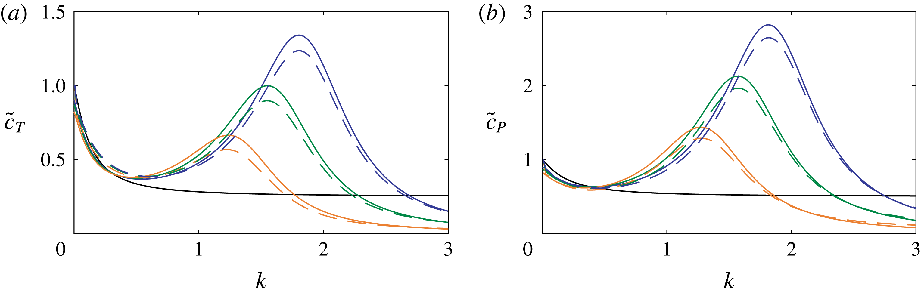
Moore (Reference Moore2017) studied the optimal thrust configuration for thrust production of flapping wings in forward flight due to chordwise flexibility. He solves the coupled one-dimensional linear beam and potential flow equations using a Chebyshev collocation iterative method, a semi-analytical approach. The normalized cycle-averaged thrust $\langle T^{\prime }\rangle$ and power $\langle P^{\prime }\rangle$ versus the reduced frequency are shown in figure 3. The black line represents the rigid wing, $\unicode[STIX]{x1D6F1}_{1}=\infty ,$ and the three coloured lines represent different stiffness, $\unicode[STIX]{x1D6F1}_{1}=5/6,5/4$ and $5/3$ . Only results near the first resonance are shown, because flapping flyers typically flap their wings at a frequency far below their wing’s first natural frequency (Moore Reference Moore2017).

It is observed that the greatest difference occurs near resonance where deformations are large, which may imply that any numerical error in Moore’s (Reference Moore2017) solution would be amplified with respect to the rate of deformations. Nonetheless, there is considerably good agreement between the two solutions, with the advantage of the current model being an exact analytical model and not requiring an iterative solver.

Figure 2.

Stability of cantilever plates. (a) Stability boundary $U_{f}^{\ast }$ and (b) flutter frequency ratio $f_{f}/f_{1}$ in terms of the mass ratio $M^{\ast }$ ; grey: Guo & Païdoussis (Reference Guo and Païdoussis2000), black: Eloy et al. (Reference Eloy, Lagrange, Souilliez and Schouveiler2008) following the method of Kornecki et al. (Reference Kornecki, Dowell and O’Brien1976), orange: Watanabe et al. (Reference Watanabe, Isaogai, Suzuki and Sugihara2002), green: Breuker et al. (Reference Breuker, Abdalla and Gürdal2008) and blue: current model ( $N=4$ , $M=20$ ).

Figure 3.

Propulsion performance of flexible wings in forward flight due to chordwise flexibility. (a) Mean thrust coefficient $\tilde{c}_{T}=\langle T^{\prime }\rangle /(2\unicode[STIX]{x03C0}^{3}\unicode[STIX]{x1D70C}_{f}(fh_{a})^{2}c)$ and (b) mean power coefficient $\tilde{c}_{P}=\langle P^{\prime }\rangle /(2\unicode[STIX]{x03C0}^{3}\unicode[STIX]{x1D70C}_{f}U_{\infty }(fh_{a})^{2}c)$ versus reduced frequency $k$ ; blue: $\unicode[STIX]{x1D6F1}_{1}=5/6$ , green: $\unicode[STIX]{x1D6F1}_{1}=5/4$ , orange: $\unicode[STIX]{x1D6F1}_{1}=5/3$ , dashed lines: Moore (Reference Moore2017) and solid lines: current model ( $N=4$ , $M=20$ ).

5 Concluding remarks

An analytical solution to the unsteady aeroelastic response of an elastic plate in axial potential flow has been presented. The key enabling step was to express the beam eigenfunctions in a Chebyshev expansion in the aerodynamic model. The generalized aerodynamic force was derived exactly in terms of the unknown temporal solution, resulting in an infinite number of non-local second-order linear ordinary differential equations, which can be solved using analytical methods. Exact expressions have been obtained for the generated lift, thrust and required input power. The flutter boundaries, obtained by the current model’s homogeneous solution, and the flexible flapping wing aerodynamics, obtained by the inhomogeneous solution, show good agreement with the results from the literature.

Supplementary material

Supplementary material is available at https://doi.org/10.1017/jfm.2018.264.

References

Bisplinghoff, R. L., Ashley, H. & Halfman, R. L. 1996 Aeroelasticity. Dover Publications.Google Scholar

Breuker, R. D., Abdalla, M. M. & Gürdal, Z. 2008 Flutter of partially rigid cantilevered two-dimensional plates in axial flow. AIAA J. 46 (4), 936–946.CrossRef Google Scholar

Eloy, C., Lagrange, R., Souilliez, C. & Schouveiler, L. 2008 Aeroelastic instability of cantilevered flexible plates in uniform flow. J. Fluid Mech. 611, 97–106.Google Scholar

Glauert, H. 1926 The Elements of Aerofoil and Airscrew Theory. Cambridge University Press.Google Scholar

Guo, C. Q. & Païdoussis, M. P. 2000 Stability of rectangular plates with free side-edges in two-dimensional inviscid channel flow. Trans. ASME J. Appl. Mech. 67, 171–176.Google Scholar

Huang, L. 1995 Flutter of cantilevered plates in axial flow. J. Fluids Struct. 9 (2), 127–147.Google Scholar

Kang, C.-K., Aono, H., Cesnik, C. E. S. & Shyy, W. 2011 Effects of flexibility on the aerodynamic performance of flapping wings. J. Fluid Mech. 689, 32–74.Google Scholar

von Karman, T. & Burgers, J. M. 1935 General Aerodynamic Theory – Perfect Fluids (ed. Durand, W. F.), Aerodynamic Theory, vol. 2, pp. 1–24. Springer.Google Scholar

Katz, J. & Plotkin, A. 2001 Low-Speed Aerodynamics, 2nd edn.. Cambridge University Press.Google Scholar

Kornecki, A., Dowell, E. H. & O’Brien, J. 1976 On the aeroelastic instability of two-dimensional panels in uniform incompressible flow. J. Sound Vib. 47 (2), 163–178.Google Scholar

Küssner, H. G. & Schwarz, I.1941 The oscillating wing with aerodynamically balanced elevator. Tech. Rep. No. 991. National Advisory Committee for Aeronautics.Google Scholar

Landahl, M. T. & Stark, V. J. E. 1968 Numerical lifting-surface theory – problems and progress. AIAA J. 6 (11), 2049–2060.Google Scholar

Moore, M. N. J. 2017 A fast chebyshev method for simulating flexible-wing propulsion. J. Comput. Phys. 345, 792–817.Google Scholar

Shelley, M. J. & Zhang, J. 2011 Flapping and bending bodies interacting with fluid flows. Annu. Rev. Fluid Mech. 43, 449–465.Google Scholar

Theodorsen, T.1935 General theory of aerodynamic instability and the mechanism of flutter. Tech. Rep. No. 496. National Advisory Committee for Aeronautics.Google Scholar

Timoshenko, S. P. 2017 Vibration Problems in Engineering, 5th edn. Dead Authors Society.Google Scholar

Walker, W. P. & Patil, M. J. 2014 Unsteady aerodynamics of deformable thin airfoils. J. Aircraft 51 (6), 1673–1680.Google Scholar

Watanabe, Y., Isaogai, K., Suzuki, S. & Sugihara, M. 2002 A theoretical study of paper flutter. J. Fluids Struct. 16 (4), 543–560.Google Scholar

Watkins, C. E., Woolston, D. S. & Cunningham, H. J.1959 A systematic kernel function procedure for determining aerodynamic forces on oscillating or steady finite wings at subsonic speeds. Tech. Rep. No. 48. National Aeronautics and Space Administration.Google Scholar

Figure 1.Schematic of case set-up.

Table 1.Chebyshev coefficient summations for the $i\text{th}$ beam eigenfunction.

Figure 2.Stability of cantilever plates. (a) Stability boundary $U_{f}^{\ast }$ and (b) flutter frequency ratio $f_{f}/f_{1}$ in terms of the mass ratio $M^{\ast }$; grey: Guo & Païdoussis (2000), black: Eloy et al. (2008) following the method of Kornecki et al. (1976), orange: Watanabe et al. (2002), green: Breuker et al. (2008) and blue: current model ($N=4$, $M=20$).

Figure 3.Propulsion performance of flexible wings in forward flight due to chordwise flexibility. (a) Mean thrust coefficient $\tilde{c}_{T}=\langle T^{\prime }\rangle /(2\unicode[STIX]{x03C0}^{3}\unicode[STIX]{x1D70C}_{f}(fh_{a})^{2}c)$ and (b) mean power coefficient $\tilde{c}_{P}=\langle P^{\prime }\rangle /(2\unicode[STIX]{x03C0}^{3}\unicode[STIX]{x1D70C}_{f}U_{\infty }(fh_{a})^{2}c)$ versus reduced frequency $k$; blue: $\unicode[STIX]{x1D6F1}_{1}=5/6$, green: $\unicode[STIX]{x1D6F1}_{1}=5/4$, orange: $\unicode[STIX]{x1D6F1}_{1}=5/3$, dashed lines: Moore (2017) and solid lines: current model ($N=4$, $M=20$).