



1. Introduction and main results
We consider continuous-state branching processes (or CB processes for short) with competition in a Lévy environment. A process of this type is a  $[0,\infty]$-valued strong Markov process with càdlàg paths which is the unique strong solution of the following stochastic differential equation (SDE):
 \begin{align}Z_t&=x+b\int_0^t Z_s\textrm{d} s-\int_0^t g(Z_s) \textrm{d} s +\sqrt{2{\gamma^2}}\int_0^t \int_{0}^{Z_s}W(\textrm{d} s, \textrm{d} u)\nonumber\\[3pt]&\quad +\int_0^t\int_{(0,\infty)} \int_0^{Z_{s-}}z\widetilde{N}(\textrm{d} s, \textrm{d} z, \textrm{d} u)+\int_0^t Z_{s-}\textrm{d} S_s,\end{align}
where g is a function on  $[0,\infty)$ with
 $g(0)=0$,
 $W(\textrm{d} s, \textrm{d} u)$ is a time–space Gaussian white noise on
 $(0,\infty)^2$ with intensity
 $\textrm{d} s \textrm{d} u$,
 $N(\textrm{d} s,\textrm{d} z,\textrm{d} u)$ is a Poisson random measure independent of W whose intensity is
 $\textrm{d} s\mu(\textrm{d} z)\textrm{d} u$, with
 $\mu$ a measure concentrated on
 $(0,\infty)$ satisfying
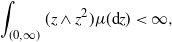 \begin{equation}\int_{(0, \infty)}(z\land z^2)\mu(\textrm{d} z)<\infty,\end{equation}
 $\widetilde{N}$ is the compensated measure associated with N (see [Reference Ikeda and Watanabe14, Chapter II] for a proper definition of the compensated Poisson integral), and S is a Lévy process with no negative jumps smaller than
 $-1$ which is independent of W and N. The Lévy process S can be written as
 \begin{equation}S_t= \sigma B^{({\rm e})}_t +\int_0^t \int_{(-1,1)^c} ({\rm e}^z-1)N^{({\rm e})}({\textrm{d} s},{\textrm{d} z})+\int_0^t \int_{(-1,1)} ({\rm e}^z-1)\widetilde{N}^{({\rm e})}({\textrm{d} s},{\textrm{d} z}),\end{equation}
where  $ \sigma\geq 0$,
 $B^{({\rm e})}=(B^{({\rm e})}_t,t\ge 0 )$ is a standard Brownian motion and
 $N^{({\rm e})}$ denotes a Poisson random measure, independent of
 $B^{({\rm e})}$, taking values on
 $\mathbb{R}_+\times \mathbb{R}$ with intensity
 ${\textrm{d} s} \pi({\textrm{d} z})$ satisfying
 \begin{equation} \int_{\mathbb{R}\setminus\{0\}} (1\land z^2) \pi(\textrm{d} z)
< \infty, \end{equation}
and  $\widetilde{N}^{({\rm e})}$ denotes the compensated version of
 $N^{({\rm e})}$. Notice that a linear term could be added in the definition of S in (3). All results would be identical since, from a mathematical point of view, this is equivalent to changing the value of b. For the convenience of the reader, such a term is thus not added in this paper.
The existence and uniqueness of the SDE (1) follows from [Reference Palau and Pardo25, Theorem 1, identity (8)]. The case  $g\equiv 0$ corresponds to a CB process in a Lévy environment, which was deeply studied, independently, in [Reference He, Li and Xu13, Reference Palau and Pardo25].
If the Lévy process S is just a linear drift (or equals 0), the strong solution of (1) corresponds to a CB process with competition. Such a family of processes has been considered recently by several authors; see, for instance, [Reference Ba and Pardoux2, Reference Berestycki, Fittipaldi and Fontbona7, Reference Foucart11, Reference Lambert18, Reference Le19, Reference Ma24, Reference Pardoux26], to name but a few. In the seminal paper [Reference Lambert18], Lambert introduced and studied the so-called logistic branching process, i.e.  $g(x)=cx^2$ for
 $x\ge 0$ and
 $c>0$. Lambert used a Lamperti-type representation (random time change) and then deduced the long-term behaviour of this process. More general competition mechanisms were considered in [Reference Ba and Pardoux2] in the case where the branching mechanism is of the form
 $\psi(u)=\gamma^2 u^2$ for
 $u\ge 0$, which is associated with Feller diffusions; see also [Reference Pardoux26, Chapter 8]. Actually, they allow the competition mechanism g to be a continuous function and not necessarily monotone, and they provide a necessary and sufficient condition for the process to become extinct. In this setting, if g is negative, the competition mechanism can be interpreted as cooperation in the sense of [Reference González-Casanova and Pardo12].
CB processes with competition in a random environment also arise as the scaling limit of discrete population models in random environment (DPREs); see, for instance, [Reference Bansaye, Caballero and Méléard4, Theorem 4.4]. DPREs describe the dynamics of populations where, at each generation, individuals reproduce independently of each other with the same offspring distribution, which depends on the population size and on an external random environment. When there is no interaction, i.e. the reproduction law only depends on the environment, DPREs are reduced to branching processes in a random environment (BPREs). These processes were introduced in [Reference Smith and Wilkinson27] and then deeply studied by several authors (see [Reference Afanasyev, Böinghoff, Kersting and Vatutin1, Reference Böinghoff, Dyakonova, Kersting and Vatutin8] and references therein). Scaling limits of BPREs in the finite-variance case were conjectured in [Reference Keiding16], which introduced Feller diffusions in a random environment. This conjecture was proved in [Reference Kurtz17], and recently in [Reference Bansaye, Caballero and Méléard4, Reference Bansaye and Simatos6] in more general cases.
Here, we assume that the measure  $\mu$ satisfies the integral condition (2) and that the function
 $g\in C^1$ is non-negative and non-decreasing. It is important to note that we may relax this last hypothesis by only assuming that there exist
 $\theta\ge 0$ such that
 \begin{equation}\textrm{the map}\ x\mapsto (\theta -b)x+g(x) \ \textrm{is non-negative and non-decreasing.}\end{equation}
In this case, the same calculations can be performed by setting  $\tilde b=\theta$ and
 $\tilde g\equiv(\theta-b){\rm Id}+g$ (where Id denotes the identity function), and studying the SDE associated with
 $\tilde b$ and
 $\tilde g$. For simplicity of exposition, we assume directly that
 $g\in C^1$ is non-negative and non-decreasing.
The integrability condition (2) and the assumptions on g are necessary to understand the long-time behaviour of the process Z, and in particular the event of extinction, for instance when  $g\equiv 0$, i.e. Z is a CB process in a Lévy environment, and under (2) the process Z does not explode and the event of extinction is well understood (see, for instance, [Reference Bansaye, Pardo and Smadi5, Lemma 7], [Reference He, Li and Xu13, Section 3], and [Reference Palau and Pardo25, Section 4]).
Our aim is to study the property of coming down from infinity for the process Z. In order to do so, knowledge of the event of extinction is required. We study the extinction event by using a comparison criterion for CB processes with competition in a Lévy environment. Such a comparison result is important for what follows and is a direct consequence of [Reference Dawson and Li9, Theorem 2.2], where the finite-mean case is treated. Here, we note that Z may have infinite mean due to the environment (recall that the Lévy measure  $\pi$ satisfies (4)). For simplicity, we state the comparison result and provide its proof below (see Proposition 1).
For simplicity of exposition, we denote by Z(x) the unique strong solution of (1) starting from  $x>0$, and by
 $\mathbb{P}_x$ its law. We may drop the notation (x) when there is no confusion. The first time Z(x) hits 0 is
 $T^{(x)}_0=\inf\{t\geq 0, Z_t(x)=0\}$, with the convention that
 $\inf\{\emptyset\}=\infty$. We also introduce the CB process in a Lévy environment
 $ Z^\sharp(x)=(Z^\sharp_t(x), t\ge 0)$ as the unique strong solution of (1) with
 $g\equiv 0$ starting from
 $x\geq 0$. We denote its law by
 $\mathbb{P}^\sharp_x$.
Proposition 1. Assume that the Lévy measure  $\mu$ satisfies (2). For
 $y\ge x\ge 0$, Z(x) is stochastically dominated by Z(y), i.e.
 \[\mathbb{P}\big(Z_t(x)\le Z_t(y)\ \textit{for\ all}\ t\ge 0\big)=1.\]
Moreover, the process Z(x) is stochastically dominated by  $ Z^\sharp(y)$.
Let us recall that the branching mechanism associated with Z is characterised by
 \begin{equation*} \psi(\lambda)=-b\lambda+\gamma^2 \lambda^2+\int_{(0,\infty)}\big({\rm e}^{-\lambda x}-1+\lambda x\big)\mu(\textrm{d} x),\qquad \text{for all } \lambda \geq 0,\end{equation*}
where the parameters  $(b, \gamma, \mu)$ are the same as in (1). According to [Reference He, Li and Xu13], Grey’s condition, i.e.
 \begin{equation}\int^\infty \frac{\textrm{d} u}{\psi(u)}<\infty,\end{equation}
is necessary and sufficient for CB processes in a Lévy environment to become extinct with positive probability (see [Reference He, Li and Xu13, Theorem 4.1]). From the latter and Proposition 1, we deduce the following result, where we denote the sets of bounded measurable and bounded continuous functions on  $[0,\infty)$ by
 $\mathcal{B}_b([0,\infty))$ and
 $C_b([0,\infty))$, respectively.
Corollary 1. Assume that the Lévy measure  $\mu$ satisfies (2) and that
 $g\in C^1$ is non-negative and non-decreasing. If the branching mechanism
 $\psi$ satisfies Grey’s condition (6), then the process Z(x) becomes extinct with positive probability and its semigroup
 $(\texttt{P}_t, t\ge 0)$ is strong Feller, in the sense that for any
 $f\in \mathcal{B}_b([0,\infty))$,
 $\texttt{P}_t\, f\in C_b([0,\infty))$ for
 $t\ge 0$.
In particular, the process is a  $C_b$ Feller, i.e.
(i) for any
 $f\in C_b([0,\infty))$, $\texttt{P}_t\, f\in C_b([0,\infty))$ for $t\ge 0$; and
(ii) for any
$f\in C_b([0,\infty))$ and $x\ge 0$, $\texttt{P}_t\, f(x)\to f(x)$ as t goes to 0.






For our last, and main, result, we assume that Grey’s condition is fulfilled. Hence, the CB processes with competition in a Lévy environment that we are considering here become extinct with positive probability and are  $C_b$ Feller.
The result provides a sufficient condition on the competition mechanism so that the processes come down from infinity, even for favourable environments. Coming down from infinity has been observed and studied by several authors in branching processes with interactions with no negative jumps, see for instance [Reference González-Casanova and Pardo12, Reference Lambert18, Reference Li22, Reference Li, Yang and Zhou23, Reference Pardoux26], and also for some jump diffusions in [Reference Bansaye3]. Formally, we define the property of coming down from infinity in the sense that  $\infty$ is a continuous entrance point, i.e.
 \[\lim_{M\to \infty}\lim_{x\to \infty}\mathbb{P}_x(T_M<t)=1 \qquad \textrm{for all} \ t>0,\]
where  $T_M=\inf\{t\ge 0\,{:}\, Z_t\le M\}$ (assuming that
 $\inf\{\emptyset\}=\infty$), and that the original process can be extended into a
 $C_b$ Feller process on
 $[0,\infty]$. In other words, its semigroup satisfies conditions (i) and (ii) of Corollary 1 for any function
 $f\in C_b([0,\infty))$ with a limit at
 $\infty$ (see, for instance, [Reference Kallenberg15, Theorem 20.13] for the diffusion case).
Let us now state our main result.
Theorem 1. Assume that the Lévy measure  $\mu$ satisfies (2) and that
 $g\in C^1$ is non-negative and non-decreasing. Suppose also that there exists
 $z_0 >0$ such that
 $g(z_0)>0$ and
 \begin{equation} \int_{z_0}^{\infty} \frac{\textrm{d} y}{g(y)}<\infty. \end{equation}
If Grey’s condition (6) holds, then
 \begin{equation}\sup_{x>0}\mathbb{E}_x[T_0]<\infty,\end{equation}
the boundary point  $\infty$ is a continuous entrance point, and the process Z comes down from infinity.
Observe that the condition on the competition parameter (7) is so strong that the process becomes extinct regardless of the long-time behaviour of the environment (see (8)). We also note that (8) was obtained in [Reference Le19] for fixed environments using similar conditions for the competition mechanism g, i.e. with (5) and (7). Indeed, condition (5) is equivalent to
 \[bu-g(x+u)+g(x)\le \theta u, \qquad \textrm{for}\ u\ge 0,\]
which is the same as condition (H1) in [Reference Le19] with  $f(x)=bx-g(x)$, and condition (7) here is equivalent to
 $\int^\infty \frac{\textrm{d} w}{|f(w)|}<\infty$, according to [Reference Le and Pardoux20, Lemma 2.3].
Moreover, the previous result can be applied to the particular case when the competition mechanism is logistic (i.e.  $g(x)=cx^2$) and the random environment is driven by a Brownian motion. Actually, further explicit computations can be carried out for the Laplace transform of the extinction time under
 $\mathbb{P}_\infty$, the law of the process starting from
 $\infty$; see [Reference Leman and Pardo21] for further details.
The remainder of this note is devoted to the proofs.
2. Proofs
In order to prove Proposition 1, we introduce the following stochastic processes as unique strong solutions of the SDEs. For  $i=1,2$, we let
 \begin{align*}Z^{(i)}_t&=Z^{(i)}_0+\int_0^tg_i(Z^{(i)}_s)\textrm{d} s+\sqrt{2\gamma^2}\int_0^t \int_{0}^{Z^{(i)}_s}W(\textrm{d} s, \textrm{d} u)\nonumber\\[3pt]&\quad +\int_0^t\int_{(0,\infty)} \int_0^{Z^{(i)}_{s-}}z\widetilde{N}(\textrm{d} s, \textrm{d} z, \textrm{d} u)+\int_0^t Z^{(i)}_{s-}\textrm{d} S^{(i)}_s,\end{align*}
where
 \begin{equation}S^{(i)}_t= \sigma B^{({\rm e})}_t +\int_0^t \int_{(-1,1)^c} (h_i(z)-1)N^{({\rm e})}({\textrm{d} s},{\textrm{d} z})+\int_0^t \int_{(-1,1)} ({\rm e}^z-1)\widetilde{N}^{({\rm e})}({\textrm{d} s},{\textrm{d} z}),\end{equation}
with  $g_1(z)\ge g_2(z)$ for
 $z\ge 0$, and
 $h_1(z)\ge h_2(z)\geq 0$ for
 $z\in \mathbb{R}$. We also assume that, for each
 ${m\ge 0}$, there is a non-decreasing concave function
 $z\mapsto r_m(z)$ on
 $\mathbb{R}_+$ satisfying
 $\int_{0+} r_m(z)^{-1}\textrm{d} z=\infty$ and, for
 $i=1,2$,
 \begin{equation*} |g_i(x)-g_i(y)|+|x-y|\int_{(-1,1)^c}\big(|h_i(z)-1|\land m\big)\pi(\textrm{d} z)\le r_m(|x-y|) \end{equation*}
for every  $0\le x, y\le m$. According to [Reference Palau and Pardo25, Proposition 1], the previous SDEs possess unique positive strong solutions that we denote by
 $Z^{(i)}$ for
 $i=1,2$.
Lemma 1. If  $Z^{(1)}_0\ge Z^{(2)}_0$, then, almost surely (a.s.),
 \[\mathbb{P}\big(Z^{(2)}_t\le Z^{(1)}_t \textrm{ for all } t\ge 0\big)=1.\]
Proof. Let  $\tau_m=\inf\{t\ge 0\,{:}\, Z^{(1)}_s\ge m \textrm{ or } Z^{(2)}_s\ge m\}$ for
 $m\ge 1$. According to the proof of [Reference Palau and Pardo25, Proposition 1], for
 $i=1, 2$ we have
 $Z^{(i)}_t=Z^{(i, m)}_t$ for
 $t<\tau_m$, where
 $Z^{(i, m)}$ is the unique strong solution to
 \begin{align*}Z^{(i, m)}_t&=Z^{(i)}_0+\int_0^tg_i(Z^{(i, m)}_s\land m)\textrm{d} s+\sqrt{2\gamma^2}\int_0^t \int_{0}^{Z^{(i, m)}_{s-}\land m}W(\textrm{d} s, \textrm{d} u)\nonumber\\[3pt] &\quad+\int_0^t\int_{(0,\infty)} \int_0^{Z^{(i, m)}_{s-}\land m}(z\land m)\widetilde{N}(\textrm{d} s, \textrm{d} z, \textrm{d} u)+\int_0^t \big(Z^{(i, m)}_{s-}\land m\big)\textrm{d} S^{(i)}_s,\end{align*}
with  $S^{(i)}$ defined by (9). In other words, for
 $m\ge 1$ we have
 \[\mathbb{P}\left(Z^{(1)}_t\ge Z^{(2)}_t, \textrm{ for all} \,\, t<\tau_m\right)=\mathbb{P}\left(Z^{(1, m)}_t\ge Z^{(2, m)}_t, \textrm{ for all } \,\, t<\tau_m\right)\!.\]
Then, a direct application of [Reference Dawson and Li9, Theorem 2.2] implies that the latter probability equals 1. The proof is completed by taking m to  $\infty$.
Proof of Proposition 1. The first statement follows directly from Lemma 1 by taking
 \[g_1(z)=g_2(z)=bz-g(z) \textrm{ for } z\ge 0\quad \textrm{and}\quad h_1(z)=h_2(z)={\rm e}^{z} \textrm{ for } z\in \mathbb{R}.\]
For the second statement, we recall that the competition mechanism g is non-negative and non-decreasing, implying that we can take  $g_1(z)=b z$,
 $g_2(z)=bz-g(z)$, and
 $h_1(z)=h_2(z)={\rm e}^{z}$. Again from Lemma 1, we deduce that the process Z(x) is stochastically dominated by
 $ Z^\sharp(y)$ for
 $y\ge x$.
Proof of Corollary 1. The first part of this result follows from the previous proposition and [Reference He, Li and Xu13, Theorem 4.1], where it was deduced that  $Z^\sharp(x)$ becomes extinct with positive probability.
It remains to deduce that the process Z(x) is strong Feller under Grey’s condition (6). With this purpose in mind, we introduce, for  $0\leq x\leq y$,
 \[T^{(x,y)}=\inf\{t\ge 0\,{:}\, Z_t(x)=Z_t(y)\}.\]
From the Markov property,  $Z_t(x)=Z_t(y)$ a.s. for any
 $t\geq T^{(x,y)}$. Thus, for any
 $f\in \mathcal{B}_b([0,\infty))$, we have
 \begin{equation}\begin{split}\big|\texttt{P}_t\, f(y)-\texttt{P}_t\, f(x)\big|&\le \mathbb{E}\left[\big|f(Z_t(y))-f(Z_t(x))\big|\textbf{1}_{\{t<T^{(x,y)}\}}\right]\\&\le2 \|\,f\|_{[0,\infty)} \mathbb{P}(t<T^{(x,y)}), \end{split}\end{equation}
where  $(\texttt{P}_t, t\geq 0)$ denotes the semigroup associated with the process Z and
 $\|\cdot\|_{[0,\infty)}$ denotes the supremum norm on
 $[0,\infty)$. Next, we define
 $\Gamma_t^{(x,y)}\coloneqq Z_t(y)-Z_t(x)$ for
 $ t\ge 0$. From Proposition 1, it is clear that
 $\Gamma_t^{(x,y)}\geq 0$ a.s. for any
 $t\geq 0$. Moreover, it satisfies
 \begin{align}\Gamma^{(x,y)}_t&= y-x+b\int_0^t \Gamma^{(x,y)}_s\textrm{d} s +\sqrt{2\gamma^2} \int_0^t \int_0^{\Gamma^{(x,y)}_s}W^\prime(\textrm{d} s, \textrm{d} u)\nonumber\\[3pt] &\quad-\int_0^t G_{Z_t(x)}(\Gamma^{(x,y)}_s) \textrm{d} s+\int_0^t\int_{(0,\infty)} \int_0^{\Gamma^{(x,y)}_{s-}}z\widetilde{N}^{\prime}(\textrm{d} s, \textrm{d} z, \textrm{d} u)+\int_0^t \Gamma^{(x,y)}_{s-}\textrm{d} S_s,\end{align}
where  $G_x(z)\coloneqq g(x+z)-g(x)$ is a non-decreasing continuous and non-negative function on
 $[0,\infty)$,
 \[W^\prime(\textrm{d} s, \textrm{d} u)\coloneqq W(\textrm{d} s, \textrm{d} u +Z_s(x))\]
is a Gaussian white noise with intensity  $\textrm{d} s \textrm{d} u$, and
 \[\widetilde{N}^{\prime}(\textrm{d} s, \textrm{d} z, \textrm{d} u)\coloneqq \widetilde{N}(\textrm{d} s, \textrm{d} z, \textrm{d} u+Z_s(x))\]
is a Poisson random measure with intensity  $\textrm{d} s\mu(\textrm{d} z) \textrm{d} u$. Again using Proposition 1, we deduce that
 \begin{equation}\mathbb{P}\left(\Gamma^{(x,y),\sharp}_t\ge \Gamma^{(x,y)}_t \textrm{ for all } t\ge 0\right)=1,\end{equation}
where the process  $\Gamma^{(x,y), \sharp}$ is the unique strong solution of (11) but with
 $G_x(z)\equiv 0$ for any
 $x,z\in [0,\infty)$. Observe that
 $\Gamma^{(x,y), \sharp}$ has the same law as
 $ Z^\sharp(y-x)$, and [Reference He, Li and Xu13, Theorem 4.1] thus implies that the former hits 0 with positive probability and that 0 is an absorbing boundary. In addition to (10) and (12), we have
 \[\begin{split}\big|\texttt{P}_t\, f(y)-\texttt{P}_t\, f(x)\big|&\le 2\|\,f\|_{{[0,\infty)}} \mathbb{P}^\sharp_{y-x}(T_0>t)\\[3pt]&\le 2\|\,f\|_{{[0,\infty)}} \mathbb{E}\left[1-{\rm e}^{-(y-x)v_t(0,\infty, K)}\right]\!,\end{split}\]
where  $v_t(0,\infty,K)$ is a functional of the auxiliary Lévy process K which is defined by
 \begin{multline*}K_t=bt-\left( \frac{\sigma^2}{2}+\int_{(-1,1)} ({\rm e}^z-1-z)\pi(\textrm{d} z)\right) t+ \sigma B^{({\rm e})}_t \\+\int_0^t \int_{(-1,1)^c} zN^{({\rm e})}({\textrm{d} s},{\textrm{d} z})+\int_0^t \int_{(-1,1)} z\widetilde{N}^{({\rm e})}({\textrm{d} s},{\textrm{d} z}), \qquad t\ge 0.\end{multline*}
Moreover, we have
 \[\mathbb{P}^\sharp_{y}(Z_t=0 \mid K)={\rm e}^{-yv_t(0,\infty,K)}>0 \]
(see, for instance, [Reference He, Li and Xu13, Theorems 4.1, 4.3]). In other words,  $|\texttt{P}_t\,f(y)-\texttt{P}_t\,f(x)|$ goes to 0 as
 $|x-y|$ goes to 0, implying that
 $\texttt{P}_t\, f$ is a continuous bounded function on
 $[0, \infty)$, i.e. the semigroup
 $(\texttt{P}_t, t\ge 0)$ is strong Feller.
Finally, it is clear that the strong Feller property and the right continuity of the unique strong solution (1) implies (i) and (ii). The proof is now complete.
Finally, we prove Theorem 1.
Proof of Theorem 1. First of all, from Lemma 1, it is enough to prove our result for a process with a random environment which has no downward jumps larger than  $1-{\rm e}^{-1}$. Hence, we assume throughout this proof that Z(x) is a solution to (1) with
 \begin{equation*} S_t= \sigma B^{({\rm e})}_t +\int_0^t \int_{(1,\infty)} ({\rm e}^z-1)N^{({\rm e})}({\textrm{d} s},{\textrm{d} z})+\int_0^t \int_{(-1,1)} ({\rm e}^z-1)\widetilde{N}^{({\rm e})}({\textrm{d} s},{\textrm{d} z}).\end{equation*}
Our first step is to prove (8). To do so, we observe that a similar Lyapunov function to the one used in [Reference Le19] will work in our case. Indeed, recall that  $T_M$ denotes the first passage time for the process Z below a level
 $M>0$, i.e.
 $T_M\coloneqq \inf \{t \geq 0, Z_t\leq M\}$. As we will see below, the finiteness of the first moment of such random times will be useful for deducing our result. Our first step is to show that there exists
 $M>0$ such that
 \begin{equation} \sup_{x\geq 0} \mathbb{E}_x\big[ T_M\big] = \sup_{x\geq M} \mathbb{E}_x\big[ T_M\big] <\infty.\end{equation}
With this goal in mind, we introduce  $A>b+\overline{\pi}(1)$, where
 $\overline{\pi}(x)=\pi([x,\infty))$. According to the integral condition in (7) and [Reference Le and Pardoux20, Lemma 2.3], we have that
 \begin{equation*} \lim_{y\to +\infty} \frac{g(y)}{y}=\infty. \end{equation*}
In other words, there exists a constant  $M>(z_0+1){\rm e}$ such that
 \begin{equation}\int_{M{\rm e}^{-1}}^{\infty}\frac{\textrm{d} w}{g(w)}\leq \frac{1}{A} \quad \text{and} \quad \frac{1}{g(y)} \leq \frac{y}{g(y)}\leq \frac{1}{A}, \qquad \text{for } y\geq M{\rm e}^{-1}.\end{equation}
The constant M will be our threshold. For our purposes, we define the function G in  $C^2(\mathbb{R})$ as
 \[ G(y)=\left\{ \begin{aligned} &\int_{z_0}^y\frac{\textrm{d} w}{g(w)} &&\text{ if } y \geq z_0+1,\\& 0 && \text{ if } y\leq z_0, \end{aligned} \right. \]
and such that G is non-negative and non-decreasing. Thus, applying Itô’s formula to  $G(Z_{t\land T_M})$, we find
 \begin{eqnarray} &&\hspace*{-110pt} G(Z_{t \wedge T_M})- G(Z_0)= -t \wedge T_M + b\int_0^{t\wedge T_M} \frac{{Z_s}}{g(Z_s)} \textrm{d} s\end{eqnarray}
 \begin{eqnarray} &&\hspace*{-84pt}- \int_0^{t\wedge T_M} \frac{g'(Z_s) }{g(Z_s)^2}\left( \gamma^2 Z_s+\frac{\sigma^2}{2}Z_s^2\right){\textrm{d} s} \end{eqnarray}
 \begin{eqnarray} && +\,\sqrt{2\gamma^2} \int_0^{t\wedge T_M}\int_0^{Z_s} \frac{1}{g(Z_s)}W(\textrm{d} s, \textrm{d} u)+ \int_0^{t\wedge T_M} \frac{\sigma{Z_s}}{g(Z_s)} \textrm{d} B^{({\rm e})}_s \end{eqnarray}
 \begin{eqnarray} &&+\,\int_0^{t \wedge T_M}\int_{(0,\infty)} Z_s\left(G(Z_{s}+z)-G(Z_{s})-\frac{z}{g(Z_{s})}\right) \mu({\textrm{d} z}){\textrm{d} s}\end{eqnarray}
 \begin{eqnarray}&& +\,\int_0^{t \wedge T_M}\int_{(0,\infty)}\int_0^{Z_{s-}} [G(Z_{s-}+z)-G(Z_{s-})]\widetilde{N}({\textrm{d} s},{\textrm{d} z},{\textrm{d} u})\end{eqnarray}
 \begin{eqnarray}&&\hspace*{-40pt} +\,\int_0^{t \wedge T_M}\int_{(1,\infty)} [G({\rm e}^z Z_{s-})-G(Z_{s-})]{N}^{({\rm e})}({\textrm{d} s},{\textrm{d} z})\end{eqnarray}
 \begin{eqnarray}&& \hspace*{-40pt}+\int_0^{t \wedge T_M}\int_{(-1,1)} [G({\rm e}^z Z_{s-})-G(Z_{s-})]\widetilde{N}^{({\rm e})}({\textrm{d} s},{\textrm{d} z})\end{eqnarray}
 \begin{eqnarray}&&+\int_0^{t \wedge T_M}\int_{(-1,1)} \left(G({\rm e}^z Z_{s})-G(Z_{s})-\frac{({\rm e}^z-1)Z_s}{g(Z_s)}\right) \pi(\textrm{d} z){\textrm{d} s}.\end{eqnarray}
We take expectations, assuming that Z starts from x, on both sides of the previous identity and we study each term separately. Our aim is to prove that the expectation of  $G(Z_{t \wedge T_M})- G(x)$ may be upper-bounded by
 $\mathbb{E}_x[t\wedge T_M]$.
We start with the integral on the right-hand side of (15). From the second inequality in (14), we see that
 \begin{equation}b\mathbb{E}_x\left[\int_0^{t\wedge T_M} \frac{{Z_s}}{g(Z_s)} \textrm{d} s\right]\le\frac{b}{A} \mathbb{E}_x\left[t\wedge T_M\right].\end{equation}
Next, since  $Z_s \geq M{\rm e}^{-1}>z_0+1$ for
 $s \leq t \wedge T_M$, and since g is non-negative and non-decreasing, the expectation of (16) is non-positive. The same assumptions imply that, for any
 $x\ge z_0+1$,
 \begin{equation} G(x+z)-G(x)-\frac{z}{g(x)}\le 0, \qquad \textrm{for }z> 0.\end{equation}
In other words, the expectations of (18) and (22) are also non-positive.
For (17), studying the quadratic variation of both continuous local martingales together with the second formula in (14), we observe that both processes are real martingales. Therefore their expectations are equal to 0.
For (19), we split the interval  $(0,\infty)$ into (0, 1] and
 $(1,\infty)$. Using the inequality in (24) together with the second formula of (14), we deduce that
 \[\mathbb{E}_x\left[ \int_0^{t \wedge T_M}\int_{(0,1)}Z_{s} \Big(G(Z_{s}+z)-G(Z_{s})\Big)^2 \mu({\textrm{d} z}){\textrm{d} s} \right]\le \frac{t}{A^2}\int_{(0,1)}z^2\mu({\textrm{d} z})<\infty. \]
Similarly, we get that
 \[\mathbb{E}_x\left[ \int_0^{t \wedge T_M}\int_{[1,\infty)}Z_{s} \Big|G(Z_{s}+z)-G(Z_{s})\Big| \mu({\textrm{d} z}){\textrm{d} s} \right]\le \frac{t}{A}\int_{[1,\infty)}z\mu({\textrm{d} z})<\infty. \]
In other words, the integral of (19) restricted to (0, 1] is a square integrable martingale and the integral restricted to  $(1, \infty)$ is a martingale. Finally, the expectation of (19) equals 0.
For (20), we use Fubini’s theorem and the first inequality in (14) to deduce that
 \begin{multline*}\mathbb{E}_x\Bigg[ \int_0^{t \wedge T_M}\int_{(1,\infty)} |G({\rm e}^z Z_{s-})-G(Z_{s-})|\pi(\textrm{d} z) \textrm{d} s\Bigg] \\[3pt]\leq \overline{\pi}(1) \mathbb{E}_x\left[ \int_0^{t \wedge T_M} \int_{Z_{s}}^{\infty} \frac{\textrm{d} w}{g(w)} \textrm{d} s \right] \leq t \overline{\pi}(1) \left(\int_{M{\rm e}^{-1}}^{\infty} \frac{\textrm{d} w}{g(w)}\right)\leq \frac{t}{A} \overline{\pi}(1).\end{multline*}
In other words, (20) may be written as the sum of a martingale and a finite variation process, and, since the martingale has null expectation, we deduce that
 \begin{align}&\mathbb{E}_x\left[\int_0^{t \wedge T_M}\int_{(1,\infty)} [G({\rm e}^z Z_{s-})-G(Z_{s-})]N^{({\rm e})}({\textrm{d} s},{\textrm{d} z})\right ]\nonumber\\[3pt]&\qquad =\mathbb{E}_x\left[\int_0^{t \wedge T_M}\int_{(1,\infty)} \left[G({\rm e}^z Z_{s-})-G(Z_{s-})\right]\pi(\textrm{d} z) \textrm{d} s \right]\le\frac{\overline{\pi}(1)}{A}\mathbb{E}[t\wedge T_M].\end{align}
Finally, for (21), the fact that  $g(w) \geq Aw$ for
 $w\geq M{\rm e}^{-1}$ implies that
 \[\begin{split}\mathbb{E}&\left[ \int_0^{t \wedge T_M}\int_{(-1, 1)} \left(G({\rm e}^zZ_s)-G(Z_s)\right)^2 \pi({\textrm{d} z}){\textrm{d} s} \right]\\[3pt]& \leq \mathbb{E}\left[ \int_0^{t \wedge T_M}\int_{(-1,1)} \left(\int_{Z_{s}}^{{\rm e}^z Z_{s}} \frac{\textrm{d} w}{Aw} \right)^2 \pi({\textrm{d} z}){\textrm{d} s} \right]\leq \frac{t}{A^2} \int_{(-1,1)} z^2 \pi({\textrm{d} z}) <\infty.\end{split}\]
In other words, (21) is a square integrable martingale and its expectation is equal to 0.
Thus, putting all the pieces together (i.e. inequalities (23) and (25), the fact that the expectations of (16), (18), and (22) are non-positive, and the fact that the expectations of (17), (19), and (21) are null), we deduce that
 \begin{equation*}\begin{aligned}\mathbb{E}_x\left[ \int_x^{Z_{t\wedge T_M}} \frac{\textrm{d} w}{g(w)} \right] \leq -\left(1-\frac{b}{A}-\frac{\overline{\pi}(1)}{A}\right) \mathbb{E}_x[t\wedge T_M]. \end{aligned}\end{equation*}
Since  $A>b+\overline{\pi}(1)$, we have, for any
 $x,t\geq 0$, that
 \begin{equation} \mathbb{E}_x\Big[t\wedge T_M\Big] \leq \frac{1}{C(A)} \mathbb{E}_x\left[ \int^x_{Z_{t\wedge T_M}} \frac{\textrm{d} w}{g(w)} \right] \leq \frac{1}{C(A)} \int_{M{\rm e}^{-1}}^{\infty} \frac{\textrm{d} w}{g(w)}, \end{equation}
where  $C(A)\coloneqq (1-\frac{b\,{+}\,\overline{\pi}(1)}{A})>0$. Hence, using the monotone convergence theorem, as t goes to
 $\infty$, we deduce (13).
In order to prove that the process becomes extinct with positive probability, we first show that the time to extinction for the process Z starting from M is not almost surely infinite. We recall that we assumed that the environment has no negative jumps larger than  $1-{\rm e}^{-1}$. Using Proposition 1 (both processes with the same restriction on negative jumps of the environment), we observe that, for any
 $x\leq M$, the process Z(x) is stochastically dominated by a process
 $ Z^\sharp(x)$ which is a CB process in a Lévy random environment (without competition) with branching mechanism
 $\psi$. Since
 $\psi$ satisfies Grey’s condition, [Reference He, Li and Xu13, Theorem 4.1] guarantees that there is
 $t_0>0$ for which
 \[ 0<\mathbb{P}^\sharp_M\big( Z^\sharp_{t_0}=0\big)\leq \inf_{x \leq M}\mathbb{P}_x\big(Z_{t_0}=0\big)\coloneqq p. \]
Reasoning by recurrence and using the Markov property, we can prove that the extinction time of Z is stochastically dominated from above by an integrable random variable. To be more precise, the algorithm is as follows.
We start from  $Z_0=x$; we wait a random time
 $T_M$ until the process is below the level M. Then, the process becomes extinct before a time interval of size
 $t_0$ with probability p. If the process is not extinct after
 $T_M+t_0$, we set
 $X_1\coloneqq Z_{T_M+t_0}$ and we repeat the procedure with a process starting from
 $X_1$ according to the Markov property. Finally, we obtain an a.s. finite sequence
 $(X_i)_{i\geq 1}$ such that Z is stochastically dominated by the random variable
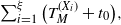 $ {\sum_{i=1}^{\xi} \big(T^{(X_i)}_{M}+t_0\big)}, $ where
 $\xi$ is a geometric random variable that counts the number of random steps before Z becomes extinct,
 $\big\{T^{(X_i)}_{M}\big\}_{i\geq 0}$ are independent of
 $\xi$, and, conditionally on the event
 $\{X_i=x\}$,
 $T^{(X_i)}_{M}$ has the same distribution as
 $T_{M}$ under
 $\mathbb{P}_x$. Hence,
 \[ \sup_{x \geq 0}\mathbb{E}_x[T_0] \leq \frac{1}{p}\left({t_0}+\sup_{x\geq 0} \mathbb{E}_x\big[T_M\Big]\right)<\infty,\]
and in particular the process becomes extinct a.s.
Let us prove that the point  $\infty$ is a continuous entrance point. From Chebyshev’s inequality, the monotone convergence theorem, and (26), we deduce that, for any
 $t>0$,
 \[\begin{aligned}\lim_{m\to \infty}\lim_{x\to \infty}\mathbb{P}_x(T_m>t)&\le \lim_{m\to \infty}\lim_{x\to \infty}\frac{\mathbb{E}_x[T_m]}{t}\\[3pt]&\leq \lim_{m\to \infty}\frac{1}{C(A)t}\int_{m{\rm e}^{-1}}^{\infty} \frac{\textrm{d} w}{g(w)}=0.\end{aligned}\]
In other words, the point  $\infty$ is a continuous entrance point.
It remains to prove the extension to a  $C_b$ Feller process on
 $[0,\infty]$. Let
 $C_b([0,\infty])$ denote the set of continuous bounded functions on
 $[0,\infty)$ with a limit at
 $\infty$, and recall that
 $(\texttt{P}_t, t\geq 0)$ denotes the semigroup associated with the process Z which is
 $C_b$ Feller on
 $[0,\infty)$.
Let  $t> 0$ be fixed. Recall, from Proposition 1, that, for any non-decreasing sequence
 $\{x_n\}_{n\ge 1}$ of strictly positive real numbers, the sequence of random variables
 $Z_t(x_n)$ is non-decreasing. Hence, it converges a.s. to a limit that we denote by
 $Z_t(\infty) \in [0,\infty]$. Then, for any
 $f\in C_b([0,\infty])$, f is bounded, and from the dominated convergence theorem we deduce that
 \[\texttt{P}_t\,f(x)=\mathbb{E}_x[\,f(Z_t)]\underset{x\to \infty}{\longrightarrow}\mathbb{E}[\,f(Z_t(\infty))].\]
We denote this limit by  $\texttt{P}_t\,f(\infty)$. Let us prove that such an extension on
 $[0,\infty]$ gives a semigroup satisfying the
 $C_b$ Feller property on
 $[0,\infty]$. The definition through a limit guarantees that
 $\texttt{P}$ remains a semigroup on
 $[0,\infty]$ and that
 $\texttt{P}_t\,f\in C_b([0,\infty])$ for
 $t\ge 0$. Thus, it remains to prove condition (ii) of Corollary 1; precisely, it remains to prove that, for any
 $f\in C_b([0,\infty])$,
 $|\texttt{P}_t\,f(\infty)-f(\infty)|\to 0 \textrm{ as } t\to 0.$ Observe that
 \[|\texttt{P}_t\,f(\infty)-f(\infty)|\le \limsup_{x\to \infty}\mathbb{E}_x\left[\left|f(Z_t)-f(\infty)\right|\right].\]
Moreover, we have
 \[\begin{split}\mathbb{E}_x\left[\left|f(Z_t)-f(\infty)\right|\right]&=\mathbb{E}_x\left[\left|f(Z_t)-f(\infty)\right|\textbf{1}_{\{T_{ x/2}\le t\}}\right]+\mathbb{E}_x\left[\left|f(Z_t)-f(\infty)\right|\textbf{1}_{\{T_{x/2}\ge t\}}\right]\\[4pt]&\le 2||f||_{[0,\infty]} \mathbb{P}_x(T_{x/2}\le t)+\sup_{y\ge \frac{x}{2}}|f(y)-f(\infty)|,\end{split}\]
where  $||\cdot||_{[0,\infty]}$ is the supremum norm over
 $[0,\infty]$. The second term is smaller as soon as x is large enough, and the first part is small as soon as t is small enough, which completes the proof of Theorem 1.
Acknowledgements
Both authors acknowledge support from the Royal Society and CONACyT-MEXICO. This work was concluded whilst JCP was on sabbatical leave holding a David Parkin Visiting Professorship at the University of Bath; he gratefully acknowledges the kind hospitality of the Department and University.


