
I. INTRODUCTION
Extrusion is well known as a high-volume production process to produce aluminum parts with fixed sectional profiles for applications in the industries of construction, automobile, aerospace, etc. It is reported that the repair and replacement of extrusion tools have significant impact on the production costs due to the failure caused by the thermo-mechanical loading of extrusion. In a typical industrial setting, up to hundreds of billets will be extruded sequentially at a frequency of 10 billets every hour, which leads to repetitive loading and unloading exerted on extrusion tools. In the extrusion process, the billet forced to flow through the tools leads to a forming load, which can be considered stable over a single stroke (dwell time). Reference Donati and Tomesani1 Moreover, a thermal balance of the die-press system will be generally obtained after an initial warm-up phase of the process (around 3-5ram strokes), keeping the die temperature remaining fairly stable during extrusion (450–500 °C). Reference Rahim, Lajis and Ariffin2 The extrusion die is under the fatigue–creep interaction due to the combined effect of stable forming load at high temperatures in multiple billet production, which plays a key role in the failure mechanisms.
The family of 5% chromium hot-work tool steels e.g., AISI H11 (X38CrMoV5-1), AISI H13 (4Cr5MoSiV1), are the commonly used materials in aluminum extrusion tools. To prolong the lifetime of extrusion dies, some efforts were made improve the high-temperature properties of these hot tool steels by modification of composition. Delagnes et al. Reference Delagnes, Lamesle, Mathon, Mebarki and Levaillant3 studied the influence of silicon content on fatigue properties of a 5% Cr tempered martensitic steel. They found that the modified AISI H11 tool steel (∼0.35 wt% silicon) exhibits improved tensile and fatigue properties at 550 °C than those of conventional ones (approximately 1 wt% silicon). Some researchers tried the new technique of laser surface remelting to improve the high-temperature properties of AISI H13. Reference Telasang, Dutta Majumdar, Padmanabham and Manna4,Reference Zhang, Lin, Cong, Kong, Zhou and Ren5 They found that the hardness of the hot tool steel surface was improved, and better fatigue resistance was found compared to the untreated one. Reference Jia, Liu, Li, Liu and Li6,Reference Telasang, Majumdar, Padmanabham and Manna7 Others were focused on the failure mechanisms of hot tool steel under its extreme working condition. Kchaou et al. Reference Kchaou, Elleuch, Desplanques, Boidin and Degallaix8 investigated the hot forging failure mechanism of AISI H13 dies and found that plastic deformation and fatigue are usually quoted as the main damage. Reggiani Reference Reggiani, Donati, Zhou and Tomesani9 studied the high-temperature behavior of AISI H11 tempered steel to determine the role that creep and fatigue play in the aluminum extrusion process. Fatigue crack propagation was also paid much attention to both at room and elevated temperatures. Reference Mosbah, Bellet and Gandin10,Reference Shah, Mabru, Baccar and Rezai-Aria11 However, the nonlinear fatigue–creep interaction of hot tool steel still lacked enough concerns, and few studies were focused on its life prediction and reliability analysis.
A large number of life prediction methods have been proposed to evaluate the fatigue, creep, and fatigue–creep life. Among these, the energy-based method can clearly describe the physical mechanism with accurate life prediction. Ductility exhaustion usually can be founded during stress relaxation in the dwell period of low-cycle fatigue tests. Reference Skelton12 The internal energy dissipates with the ductility exhaustion, which indicates the reduction of material static toughness. Reference Nikbin13 Based on that, Fan et al. Reference Fan, Shi and Tokuda14 set up an analytical approach to calculate the hysteresis energy for fatigue–creep life prediction, and the results showed good agreement. Zhu et al. Reference Zhu, Huang, He, Liu and Wang15–Reference Zhu, Lei, Huang, Yang and Peng18 has developed the energy method with several approaches to improve the life prediction accuracy such as introducing fatigue–creep damage parameter, adopting frequency separation techniques, proposing a novel viscosity-based model, and suggesting a mean stress corrected strain energy model, etc. Recently a unified ductility criterion for fatigue–creep life prediction was proposed based on the dissipated cyclic strain energy density of the high-temperature component. Reference Zhu, Yang, Huang, Lv and Wang19 Applicability and prediction accuracy of the newly proposed criterion were validated more accurately than other existing strain energy/ductility-based methods. By incorporating a reliability analysis, a probabilistic framework was also established, and a first order approximation was used to derive the safety factor for the fatigue design. Reference Zhu, Foletti and Beretta20
In the present study, a mean strain life model was proposed based on the energy conservation. Statistical analysis has been considered to illustrate the random behavior of fatigue and fatigue–creep life. A confidence interval was adopted to improve the prediction accuracy. To validate the model, a series of AISI H13 fatigue and fatigue–creep tests were conducted at 500 °C. The strain-controlled tests were used for obtaining the parameters, while the stress-controlled tests were utilized for validating the proposed model.
II. EXPERIMENTAL DETAILS
A. Material
The material investigated in the present study is AISI H13, and the cylindrical specimens were taken out of a forged ingot, of which the chemical composition is presented in Table I. To achieve a hardness of 47-49HRC (Rockwell hardness), heat treatment includes austenitising at 1020 °C for 1 h followed by nitrogen quenching, tow tempering twice at 570 °C and 550 °C, respectively, and then air cooling to room temperature. Figure 1 shows the different magnifications of the micrograph of AISI H13 after heat treatment with OM (Olympus Measuring Laser Microscope OLS4000, Olympus, Tokyo, Japan) and JEOL JSM-7800F field emission gun scanning electron microscope (SEM; JEOL Ltd., Tokyo, Japan). It can be revealed that the hardened and tempered AISI H13 tool steel (ThyssenKrupp Materials, Shanghai, China) is with large quantities of fine tempered martensite lath.
Chemical composition of hot-work steel AISI H13.

Different magnifications of the micrograph of AISI H13 (a) optical micrograph and (b) electron backscatter diffraction image.

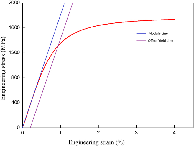
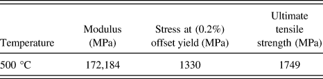
The stress–strain curve of AISI H13 hot tool steel at 500 °C is shown in Fig. 2. The high tensile strength can be found at 500 °C after heat treatment. Three tensile tests were conducted to acquire the average value of the tensile properties of AISI H13 steel, and the comparative mechanical properties at 500 °C are given in Table II.
Tensile curve of AISI H13 steel at 500 °C.

Basic mechanical properties of AISI H13 steel at 500 °C.

B. Test setup
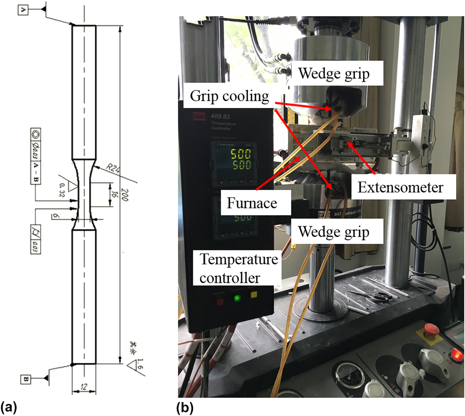
The detailed drawing of the AISI H13 specimens is shown in Fig. 3(a), and the surface of the specimens was carefully polished along the longitude direction to remove the scratches. The middle section of the specimen (16 mm) is referred to as the gauge section. All of the tests were conducted on an MTS 100-kN closed-loop servo-hydraulic testing machine with MTS Furnace 653 (MTS Systems Corporation, Eden Prairie, Minnesota) at ambient temperatures, as shown in Fig. 3(b). A clip gauge with 12.0 mm distance between the ceramic bars was used to monitor the strain, and two K-type thermocouples were directly attached to the specimen to measure the temperature. The tested temperature is started ramping to in 15 min, then soaked for 30 min at the test temperatures to ensure the uniform temperature throughout the gauge section of the specimen.
(a) Detailed drawing of the AISI H13 specimens and (b) the experimental setup.

All fully tension-compression low cycle tests with and without holding times were conducted on the specimens at an ambient temperature of 500 °C. This temperature was selected due to its application in an aluminum extrusion container. Once the temperature was achieved, the triangular loading waveform with and without tension holding times was set up in the software of Multipurpose Elite. For strain-controlled tests, the strain rate was all set as 0.01%/s. For stress-controlled tests, the load rate was all set as 400 MPa/s. A 10% drop method was suggested and considered for the failure criterion, which means that the maximum allowed stress at the cycle number is decreased by 10% from the stabilization level. The test data were collected by a PC.
III. A MEAN PLASTIC STRAIN LIFE PREDICTION BASED ON ENERGY METHOD
Various inevitable micro defects will be generated in the specimen under fatigue–creep load (e.g., dislocation, void, micro crack, etc.). These irreversible processes occur with the increase of internal energy. A local form can be derived from the law of energy conservation for the specimen under high-temperature fatigue–creep tests Reference Fan, Shi and Tokuda14 :
 $$\rho \cdot {{{\rm{d}}e} \over {{\rm{d}}t}} = \sigma \cdot \dot{\varepsilon } + {{{\rm{d}}Q} \over {{\rm{d}}t}}\quad ,$$
where e is the internal energy per mass, Q is the thermal energy per mass. Equation (1) indicates that the internal energy accumulation equals to the change of the mechanical work and heat transfer. For isothermal tests, the complicated heat exchange is related to the mechanical work to keep the temperature of the specimen constant. And thus, the right side of Eq. (1) can be given as a function of the mechanical work:
 $$\rho \cdot {{{\rm{d}}e} \over {{\rm{d}}t}} = f\left( {\sigma \cdot \dot{\varepsilon }} \right)\quad .$$
Toughness of a material can be defined as the ability to absorb energy and resist permanent deformation without fracturing. The failure occurs when the internal energy reaches a critical value. The material toughness continuously deteriorates with the increase of internal energy absorbed into the material, forming various micro defects. Since the internal energy is immeasurable, the function of mechanical work can be used to be defined as the LCF damage parameter from Eq. (2). Let ω represent a measurement of material degradation, and it can be expressed as:
 $${{{\rm{d}}\omega } \over {{\rm{d}}t}} = {{\partial \omega } \over {\partial U}} \cdot {{\partial U} \over {\partial t}} = {{\partial \omega } \over {\partial f\left( {\sigma ,\varepsilon } \right)}} \cdot {{\partial f\left( {\sigma ,\varepsilon } \right)} \over {\partial \varepsilon }} \cdot {{\partial \varepsilon } \over {\partial t}}\quad ,$$
where U represents the internal energy equaled to the function of the mechanical work f(σ, ε). Assuming that elastic deformation is reversible and does not cause the change of internal energy, the internal energy is only related to the plastic deformation. Thus, Eq. (3) can be replaced as follows:
 $${{{\rm{d}}\omega } \over {{\rm{d}}t}} = {{\partial \omega } \over {\partial f\left( {\sigma ,{\varepsilon _{\rm{p}}}} \right)}} \cdot {{\partial f\left( {\sigma ,{\varepsilon _{\rm{p}}}} \right)} \over {\partial {\varepsilon _{\rm{p}}}}} \cdot {{\partial {\varepsilon _{\rm{p}}}} \over {\partial t}} = {F_{\rm{D}}} \cdot {\dot{\varepsilon }_{\rm{p}}}\quad .$$
From Eq. (4), the process of material deterioration can be analogy as a process of doing work. The damage rate can be defined as the product of the damage force F D and the rate of the plastic strain, where F D is not a real force but a measure of the capability that mechanical work applied on the material transforms into internal energy. Integrating the damage per cycle, the amount of damage per cycle thus can be obtained:
 $${\rm{d}}D = \int {{{{\rm{d}}\omega } \over {{\rm{d}}t}}} {\rm{d}}t = \int {{F_{\rm{D}}}{\rm{d}}\varepsilon _{\rm{p}}^{{\rm{per}}}} = \left( {{F_{\rm{D}}} - \int {{\rm{d}}{F_{\rm{D}}}} } \right) \cdot \varepsilon _{\rm{p}}^{{\rm{per}}} = {F_{\rm{D}}}^\prime \cdot \varepsilon _{\rm{p}}^{{\rm{per}}}\quad ,$$
where F
D′ is the energy transformation parameter per cycle and
 $\varepsilon _{\rm{p}}^{{\rm{per}}}$
is the plastic strain per cycle.
According to Eq. (5) and the analogy mentioned above, damage evolution can also be considered as a ductility exhaustion process. The more damage that is accumulated, the more ductility is exhausted. The plastic strain under fatigue–creep interaction consists of cyclic creep strain and static creep strain, respectively. Based on the equivalent stress concept of continue damage mechanics (CDM), the plastic strain per cycle under the stress-controlled fatigue–creep condition can be generally written as Reference Wang21 :
 $$\varepsilon _{\rm{p}}^{{\rm{per}}} = {{{\rm{d}}{\varepsilon _{\rm{p}}}} \over {{\rm{d}}N}} = {\left[ {{{{\sigma _{{\rm{eqv}}}}} \over {A\left( {1 - D} \right)}}} \right]^m} = {\left[ {{{g\left( {{\sigma _{\max }},{\sigma _{\rm{m}}},{t_{\rm{h}}} \ldots } \right)} \over {A\left( {1 - D} \right)}}} \right]^m}\quad ,$$
where A and m are material constants. Cyclic strain is mainly related to σa, σmax, etc., and static creep strain is mainly caused by σmax, σm, t h, etc.; thus, the plastic strain is a complex function of these factors. Here, the equivalent stress is used to represent the coupled effect.
Substituting Eq. (6) into Eq. (5), the damage increment per cycle can be deduced:
 $${\rm{d}}D = {F_{\rm{D}}}^\prime \cdot {\left[ {{{g\left( {{\sigma _{\max }},{\sigma _{\rm{m}}},{t_{\rm{h}}} \ldots } \right)} \over {A\left( {1 - D} \right)}}} \right]^m}{\rm{d}}N\quad .$$
Integrating Eq. (7) with initial condition:
 $${\left. D \right|_{N = 0}} = {D_0}\quad {\left. D \right|_{N = {N_{\rm{f}}}}} = 1\quad ,$$
where D 0 is the initial damage, and material failure occurs when damage comes to 1, which gives
 $${N_{\rm{f}}} = {F_{\rm{D}}}^\prime \cdot {{\left( {1 - {D_0}} \right)} \over {m + 1}} \cdot {\left[ {{A \over {g\left( {{\sigma _{\max }},{\sigma _{\rm{m}}},{t_{\rm{h}}} \ldots } \right)}}} \right]^m}\quad ,$$
 $$1 - D = \left( {1 - {D_0}} \right) \cdot {\left( {1 - {N \over {{N_{\rm{f}}}}}} \right)^{{1 \over {1 + m}}}}\quad .$$
Substituting Eq. (9) into Eq. (6), the increment of plastic strain per cycle is given
 $${{{\rm{d}}{\varepsilon _{\rm{p}}}} \over {{\rm{d}}N}} = = {\left[ {{{g\left( {{\sigma _{\max }},{\sigma _{\rm{m}}},{t_{\rm{h}}} \ldots } \right)} \over {A \cdot \left( {1 - {D_0}} \right) \cdot {{\left( {1 - {N \over {{N_{\rm{f}}}}}} \right)}^{{1 \over {1 + m}}}}}}} \right]^m}\quad .$$
Some assumptions Reference Fan, Chen, Chen and Jiang22 are made that the plastic strain at half-life represents the mean plastic strain. To be more precise, the following relationship gives:
 $${\left. {{{{\rm{d}}{\varepsilon _{\rm{p}}}} \over {{\rm{d}}N}}} \right|_{N = 0.5{N_{\rm{f}}}}} = {\left[ {{{g\left( {{\sigma _{\max }},{\sigma _{\rm{m}}},{t_{\rm{h}}} \ldots } \right)} \over {A \cdot \left( {1 - {D_0}} \right) \cdot {{0.5}^{{1 \over {1 + m}}}}}}} \right]^m} = \Delta {\varepsilon _{\rm{m}}}^\alpha \quad ,$$
 $$\Delta {\varepsilon _{\rm{m}}} = {1 \over {{N_{\rm{f}}}}}\sum\limits_{i = 1}^{{N_{\rm{f}}}} {{\rm{d}}{\varepsilon _{{\rm{pi}}}}} \quad ,$$
where Δεm denoting mean strain is the mean of the plastic strain per cycle through the whole life time. By Eqs. (11) and (8), we can finally get the final simple life model, where k is the material constant:
 $${N_{\rm{f}}} = k \cdot \Delta {\varepsilon _{\rm{m}}}^{ - \alpha }\quad ,$$
 $$k = {F_{\rm{D}}}^\prime \cdot {{\left( {1 - {D_0}} \right)} \over {\left( {m + 1} \right) \cdot {{0.5}^{{m \over {m + 1}}}}}}\quad .$$
IV. STATISTICAL ANALYSIS OF THE LIFE PREDICTION MODEL
The life prediction model based on the energy method was derived from the paragraphs above. However, fatigue as well as fatigue–creep life usually exhibits a random behavior because inhomogeneity in materials inherents microstructural properties, model errors, differences in the specimen surface, and other factors. Reference Sankararaman and Mahadevan23,Reference Guida and Penta24
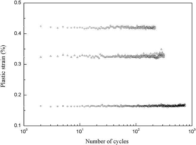
Complicated microstructure evolution with different macro performances occurs during the load process. Reference Giordana, Giroux, Alvarez-Armas, Sauzay, Armas and Kruml25,Reference Kim and Kim26 Du et al. Reference Du, Luo, Wang, Chen and Yu27 investigated the macro cyclic stress response and the microstructure evolution of AISI H11 during high-temperature fatigue tests. It shows that AISI H11 presents three stages like most metallic materials during the life time: an initial hardening phase usually covering a short number of cycles, followed by a stabilization phase covering the major part of the life time, and finally a crack propagation stage leading to a fracture. Since the dynamic balance of hardening and softening occupies most of the life time, it may be reasonable to approximate the transformation relationship in this dynamic balance stage as that of whole life. However, it cannot be promised that F D is a fixed value due to its complicated microstructure evolution and other unknown factors. It will be of great significance to take F D as a random variable that represents a random process dependent on time. Model errors also occur because the plastic strain per cycle usually varies all over the life time. Figure 4 shows the plastic strain per cycle through the whole lifetime under a load condition of 0.8%, 1.0%, 1.0% t600 s. Random phenomenon still can be found for the one specimen under a fixed load condition.
Plastic strain per cycle through whole life time under load condition of 0.8%, 1.0%, 1.0% t600 s.

Therefore the cycle life on one working condition in fact presents a set of possible different values, each with a corresponding probability instead of a single and fixed value. To model this experimental variability, a random error term is introduced in Eq. (12):
 $${N_{{\rm{fi}}}} = k \cdot \Delta {\varepsilon _{{\rm{mi}}}}^{ - \alpha } \cdot {\delta _i}\quad ,$$
where δ i is usually assumed to be distributed as a log-normal random variable with (unknown) variance independent of Δεmi. If conducting repeated tests, the errors δ i are assumed to be independent with each other.
For statistical analysis, it is usual to rewrite Eq. (13) into a logarithm expression. Arranging the following transform, the simple linear regression model is obtained:
 $${Y_i} = \beta - \alpha {x_i} + \sigma {e_i}\quad ,$$
where Y
i
= log N
fi,
 ${x_i} = {u_i} - \bar{u}$
, u
i
= log Δεmi,
 $\bar{u} = {1 \over n}\sum\limits_1^n {{u_i}}$
,
 $\beta = \log k - \alpha \bar{u}$
, and e
i
∼ N(0,1). The Y
i
is usually assumed to obey independently distribute normal random variables with mean
 ${\mu _{{x_i}}} = \beta - \alpha {x_i}$
and constant variance σ2. Thus the probability density function (PDF) of the random variable Y
i
can be given by:
 $$f\left( {{Y_i}} \right) = {1 \over {\sqrt {2\pi } \sigma }} \cdot \exp \left[ { - {1 \over {2{\sigma ^2}}}\left( {{Y_i} - \beta + \alpha {x_i}} \right)} \right]\quad .$$
After observing the couples (x i , Y i ) (i = 1, 2, …, n), the unknown parameters α and β are estimated by the maximum likelihood method, which gives:
 $$\hat{\alpha } = {{\sum\limits_{i = 1}^n {{x_i} \cdot {Y_i}} } \over {\sum\limits_{i = 1}^n {x_i^2} }}\quad \hat{\beta } = {1 \over n}\sum\limits_{i = 1}^n {{Y_i}} \quad .$$
Thus
 $\hat{\alpha }$
and
 $\hat{\beta }$
are the linear estimators, and they are linear combinations of the observed data Y
i
. Since Y
i
are normal random variables, the repeated samples also are
 $\hat{\alpha }$
and
 $\hat{\beta }$
normal random variables. They are unbiased minimum variance estimators. The minimum variance unbiased estimator of the error term is usually obtained as follows:
 $${s^2} = {{\sum\limits_{i = 1}^n {{{\left( {{Y_i} - {{\hat{\mu }}_{{x_i}}}} \right)}^2}} } \over {n - 2}}\quad ,$$
where
 ${\hat{\mu }_{{x_i}}} = \hat{\beta } - \hat{\alpha }{x_i}$
.
When sufficient data is available, these estimated parameters come to their true values. However, in case of a small sample number, the confidence level of results should be taken into consideration. Usually, the width of confidence intervals is determined by the amount of data when the confidence levels are fixed. Reference Xiong and Shenoi28 For the same confidence interval, the more data items there are, the narrower the confidence level in the statistical results will be. To calculate the confidence interval for cyclic life, the t-distribution is generally used. The following random variable obeys the t-distribution with an n − 2 degree of freedom:
 $$T = {{\left( {{{\hat{\mu }}_x} - {\mu _x}} \right)} / {{s_{{{\hat{u}}_x}}}}}\quad ,$$
where μ
x
= β − αx and
 ${s_{{\mu _x}}} = s\sqrt {{1 / n} + {{{x^2}} / {\sum\limits_{i = 1}^n {x_i^2} }}}$
. Finally, the 1 − γ two-sided equal tailed confidence interval is:
 $${\hat{\mu }_x} \pm s{t_{\gamma {\rm{/}}2;n - 2}}\sqrt {{1 / n} + {{{x^2}} / {\sum\limits_{i = 1}^n {x_i^2} }}} \quad .$$
The statistical analysis of the mean strain life model has been made. Thus it determines that the predicted life is not a fixed value but a certain two-side confidence interval with a probability of 1 − γ in which the failure life will fall in. This data-driven analysis can significantly complement the physical-based model inaccuracy due to unmeasured and unknown exogenous influences.
V. EXPERIMENTAL RESULTS
A. Fracture behavior
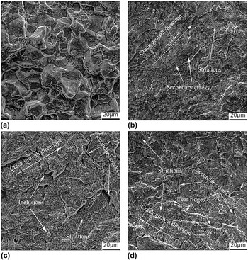
To further understand the failure mechanism of H13 under the working condition of aluminum, the fracture surfaces of creep and fatigue–creep specimens (with dwell time of 0, 10, 600 s) were observed by Scanning electron microscope (SEM). Figure 5(a) shows the fracture surface on the creep specimen that is with an inter-granular brittle fracture. The failure mechanism is probably caused by strain localization and creep cavitation forming at grain boundaries. It deteriorates the strength of grain boundaries and makes it brittle, finally leading to local grain-boundary separation with void the nucleation and propagation. Reference Yan, Zhang, Tu, Mannan, Xuan and Lin29 Figures 5(b)–5(d) show fracture surfaces of the specimen (−500 1500 MPa) with a holding time of 0, 10, and 600 s. The fatigue striations can be more clearly observed with a holding time of 600 s than that of 0 and 10 s. More secondary cracks are also found with the increase of the holding time. The phenomenon can be explained by interaction of the damage effect of fatigue and creep.
Fracture surfaces (a) creep, (b) t = 0 s, (c) t = 10 s, and (d) t = 600 s.

B. Verification of the new life model
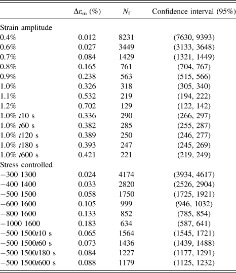
In this section, the life prediction model of Eq. (12) above will be verified by the data from experiment results of AISI H13. Table III illustrates the fatigue and fatigue–creep test results. The tests were divided into two groups. One group which consists of strain-controlled fatigue and fatigue–creep tests is utilized to fit the material constants k and α in Eq. (12). To verify the proposed model, the other stress-controlled group of fatigue tests and fatigue–creep tests were performed.
The fatigue and fatigue–creep test results.

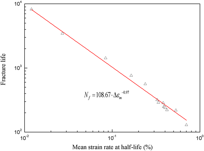
The results of fitting the numbers of failure and mean plastic strain were shown in Fig. 6. It shows that the mean plastic strain Δεm relates to N f linearly very well at a double logarithmic coordinate under both fatigue and fatigue–creep tests. The fitting material parameters k and α can be obtained, and the fitting equation of AISI H13 at 500 °C is as follows:
 $${N_{\rm{f}}} = 108.67 \cdot \Delta {\varepsilon _{\rm{m}}}^{ - 0.97}\quad ,$$
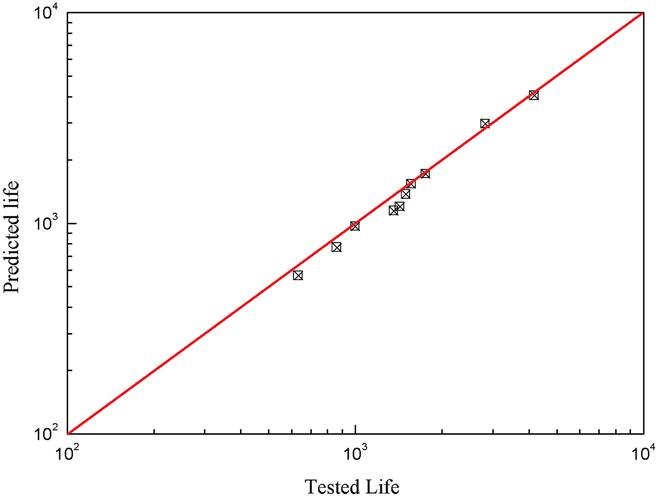
where the linear correlation coefficient R = 0.99751. Figure 7 shows the comparison of the predicted life based on proposed model and experiment stress-controlled life. Good correlations between the experimental results and predictions of the proposed model can be seen.
Fitting results of the model with strain-controlled life.

Comparison of the predicted life and experimental stress-controlled life.

From Table III, it can be found that life reduction does not seem obvious with the increase of hold time. Because the toughness of experimental material AISI H13 is high even at elevated temperatures, the accumulated static creep strain was rather smaller compared to the cyclic creep strain. Although it was rather small, the small increase of mean plastic strain and the small reduction of cyclic life still can be found with the increase of hold time, which means that the static creep strain generated during hold time influences the cyclic life.
The results show the good accuracy of life prediction. However, it is just applicable for low-cycle fatigue and fatigue–creep tests at elevated temperatures since the model was deduced from the law of energy conservation for the specimen under high temperature. Moreover, high-cycle fatigue will not be suitable using this model since there will be no or rare plastic strain existing.
C. The reliability analysis
Since life exhibits a random behavior as mentioned above, it is necessary to calculate the confidence interval. According to the collected data, the unknown parameters α and β can be obtained by Eq. (16) above:
 $$\hat{\alpha } = - 0.99\quad \hat{\beta } = - 2.88\quad .$$
Then the life range of each load condition with 1 − γ confidence can be calculated. Table III shows the calculated life intervals with a confidence level of 95%. It can be found that each experiment life falls in their life interval. However, the larger the experiment failure life is, the wider the width of the life confidence interval is. This means that the life shows a more random behavior than those lower load conditions.
The distribution function of life can be obtained from Eq. (15). The reliability can be expressed as follows:
 $$R\left( n \right) = 1 - P\left[ {n \le {N_{\rm{f}}}} \right]\quad .$$
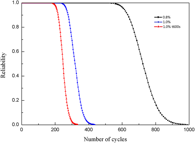
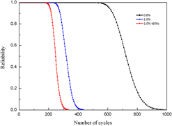
Then substituting Eq. (15), the reliability of the specimen can be calculated under a certain load condition. Figure 8 plots the time-dependent reliability curves for AISI H13 steel under three different load conditions, 0.8%, 1.0%, 1.0% t10 min, respectively. It can be clearly seen that reliability decreases with an increase in time or number of loading cycles. Moreover, the initial stage of reliability is relatively high and nearly has no decrease, which represents the long period of damage initiation. It should be noted that although the specimen has failed in this experiment, its reliability may not be zero according to the calculation. The life of reliability of zero represents the maximum life this specimen could reach.
Reliability curves for AISI H13 steel under three different load condition (0.8%, 1.0%, 1.0% t10 min).

VI. CONCLUSIONS
This article presented a new mean plastic strain model based on the energy for predicting fatigue and fatigue–creep life-time of AISI H13 (4Cr5MoSiV1). To validate the model, a series of tests of AISI H13 were performed at 500° high temperature. In addition, the reliability analysis with a classical statistical method has been made. Following conclusions can be drawn:
-
(1) The life-time model for fatigue and fatigue–creep of AISI H13 at 500 °C was obtained, and the expression was shown as:
 ${N_{\rm{f}}} = 108.67 \cdot \Delta {\varepsilon _{\rm{m}}}^{ - 0.97}$
. Besides, the results predicted by the proposed model are in a good agreement with the experimental results.
-
(2) The life interval of each load condition with 95% confidence can be calculated. The results show that larger the experiment failure life is, the wider the width of the life confidence interval is
-
(3) The curve of the number of cycles to failure at the associated probability was deduced. The life time of reliability zero can be obtained, which is usually larger than the experimental failure life.

ACKNOWLEDGMENT
This work was sponsored by National Natural Science Foundation of China (Grant No. 51405044).