2. EPISTEMIC LANDSCAPES, PROBLEM DIFFICULTY, AND THE FIENDISHNESS INDEX

Some research questions are easier to answer than others. However, what counts as a difficult problem varies from field to field, and attempts to codify and measure problem difficulty vary accordingly. In computational complexity research, a well-known line is drawn between P problems, whose answers are computable in polynomial time, and NP problems, answers for which are only verifiable in polynomial time. That is one measure of question difficulty. It also remains a notably hard open question whether P = NP. In optimization research, there are also attempts at finding a satisfactory measure for fitness functions resistant to solution by genetic algorithm and evolutionary computation. Isolation, fitness-distance correlation, fitness variance, and epistasis variance have all been proposed as measures of difficulty in this regard, but for each there are some intuitively easy cases that those measures improperly classify as hard and some intuitively hard cases they class as easy (Naudts and Kallel Reference Naudts and Kallel2000; He et al. Reference He, Reeves, Witt and Yao2007). The term ‘wicked problem’ has been applied in social policy with a set of fairly loose criteria. Novel or unique problems are said to be wicked if they have no definitive formulation, definitive solution, or even a definitive set of alternative solutions. A problem is wicked if it is a one-shot problem for which an answer cannot be generalized from other cases or generated by trial or error, and the investigation of which carries no "stopping rule" (Rittel and Webber Reference Rittel, Webber and Cross1973; Conklin Reference Conklin, Kirschner, Shum and Carr2003).

The modeling framework we present below is flexible enough to model many types of problem difficulty. In this first paper we restrict ourselves to problems that are difficult for the straightforward empirical reason that their solution may take a lot of trial-and-error to find; e.g., practical medical effectiveness, true causal pathways, how a specific protein folds, or where a treasure is buried. Some questions of this kind prove difficult because of tempting answers that are merely second- or third-best. Other questions prove particularly difficult because the answer (e.g., the best treatment, the true causal chain, the correct folding pathway, or the actual treasure location) is a “needle in a haystack,” hard to find because it is hidden in a tiny portion of the hypothesis space. For this kind of question, the shape of the epistemic terrain makes it difficult to find the right answer. We'll call a difficult problem of this type “fiendish.”

In our models, graphs are used to represent particular aspects of the epistemic structure of a problem. For a question about which dosage of an antiviral drug is most effective, hypothesized best dosages are represented on one axis. The other axis gives a measure of how good each hypothesis is – the percentage of patients who show remission at a given dosage, for example. These epistemic landscapes are similar to fitness landscapes in biology except that the height indicates epistemic fitness of a hypothesis rather than ecological fitness of a genotype.Footnote ¹We think of the epistemic landscape as giving an objective picture of the problem under investigation: it maps every possible hypothesis to the strength of the epistemic upshot of the deliverances of the world for a research investigating that hypothesis, which we can think of as the epistemic goodness of that hypothesis.

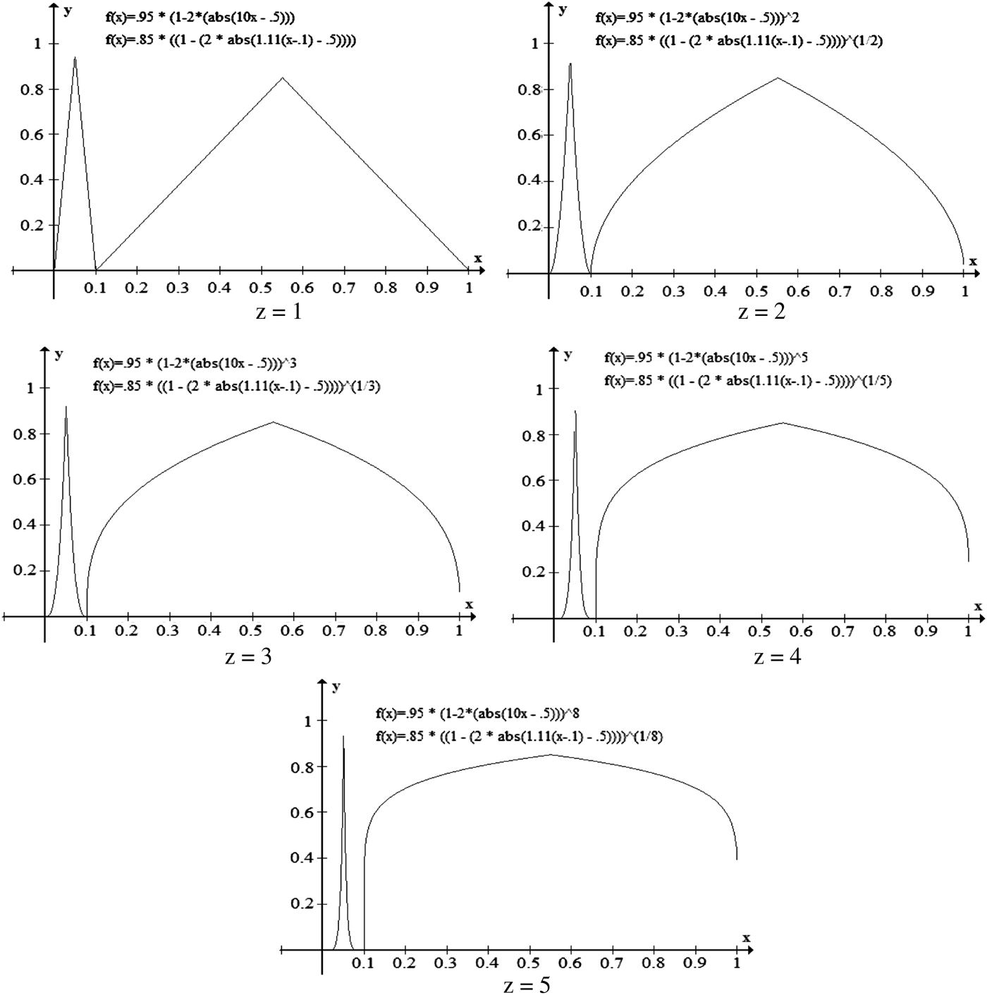
The epistemic landscape gives a “God's eye view” of the epistemic payoffs of the entire collection of hypotheses. All the individual researcher has access to is a small collection of particular points of investigation on that landscape. A researcher adopts a hypothesis by taking a value on the x-axis. Only then can he find the epistemic payoff for that hypothesis represented in the landscape. Researchers are doing better when the epistemic payoff of their hypothesis is higher, so researchers aim to adopt the hypothesis with the highest payoff. What makes a question fiendish is that the epistemically best hypothesis is hard to find. Progressively more fiendish questions are represented by the epistemic landscapes in Fig. 1. In our models, we restrict ourselves to linear representations to reduce the complexity of the model; in many cases, such as combination of two cancer treatments, an epistemic landscape will be better represented in more dimensions (Fig. 2). Empirical questions may be difficult in other regards as well (e.g., due to ambiguous, missing, or conflicting evidence), but our inquiry here is focused on fiendishness.

Fig. 1.

(colour online) An abstract representation of progressively more fiendish empirical questions.

Fig. 2.

(colour online) An idealized epistemic landscape for effectiveness of combined cancer therapies.

As the examples make clear, landscapes can contain both a global maximum peak and one or more sub-optimal local maxima. The number, location, height, and position of the maxima of the landscape can affect its fiendishness. Intuitively, finding the needle in the haystack is a more fiendish problem than finding a medium-sized object in the haystack because a searcher is less likely to happen upon the needle in the course of the search. We provide a formal measure of fiendishness that is meant to capture this idea: The fiendishness index of a landscape, relative to a number N, is the probability that for N random points on the landscape, the highest point will not be within the basin of attraction of the global maximum. The basin of attraction for a maxima is the set of points on the landscape for which simple hill-climbing will result in that maxima. Lower probabilities that the highest random point is within the highest peak's basin of attraction correspond to higher fiendishness. Alternatively stated, higher fiendishness scores correspond to landscapes on which there is a lower probability that hill-climbing from the highest randomly chosen point results in the landscape's global maximum.

There will be an uncountable number of different landscapes that have any given fiendishness index. In what follows, we focus on simple landscapes constructed in terms of just two peaks: a global maximum that takes the form of a “needle in a haystack” spike, with a height (success level) of 0.95, and a local maximum hump with a height of 0.85 (Fig. 3).

Fig. 3.

(colour online) A simple “spike and hump” epistemic landscape.

We construct our landscapes using a formula in which we can vary the curvature of the spike and hump, without varying the width of their bases. For the spike (shown between x = 0.35 and x = 0.45 in Fig. 3).

$$\,f\lpar x\rpar = 0.95\left( {1 - 2\left( {abs\left( {10x - 0.5} \right)} \right)} \right)^Z .$$

For the hump,

$$\,f\lpar x\rpar =0.85\left({1 - 2\left({abs\left({\displaystyle{{10} \over {9\lpar x - 0.1\rpar }} - 0.5} \right)} \right)} \right)^{\left({{1 \over Z}} \right)}.$$

The variable z is used in both to adjust the curvature of the spike and hump. The fiendishness index tracks the probability that the highest of N random points on the landscape will be in the basin of our global maximum. Using the formulae above, we can also think of fiendishness in terms of the “fiendishness exponent” z. Figure 4 shows the increasingly fiendish landscapes generated with these formulae for exponents 1, 2, 3, 5, and 8. Here for simplicity we exhibit the spike to the left (which does not affect the fiendishness index).

Fig. 4.

Epistemic landscapes for exponents z = 1, 2, 3, 5, and 8 showing increasing fiendishness.

Though the fiendishness exponent determines the topology of a particular class of landscapes, the particular probability of the highest of N random points falling in the basin of the global maximum will be relative to N. In other words, how improbable it will be for the highest random drop to land in the basin of the global maximum will depend on the number of random drops we are allowed. Figure 5 shows the probability of the highest drop landing in the spike area for N between 1 and 100 and for fiendishness exponents of z = 1, 3, 5, and 7. In what follows, we will focus on the comparative success of different scientific networks with the same number of agents (fixed value of N) across a range of landscapes. We vary the fiendishness index of the landscapes through changes in the parameter z, which tracks the fiendishness index when the number of agents is held fixed.

Fig. 5.

(colour online) (1 − fiendishness index) as a function of the parameter z and the number of random drops.

3. MODELING THE SOCIAL STRUCTURE OF SCIENCE

Using our epistemic landscapes, we can produce a highly idealized, simple simulation model of the social structure of a population of scientists. We consider collections of scientist agents, each of whom has a hypothesis, which we model as the agent having a location on the x-axis of the landscape. Agents are also connected to other agents. At each round of the model, agents receive feedback from the landscape and other agents, and then they change their hypothesis based on the feedback. The feedback consists of the epistemic fitness (the y-value) of their current hypothesis and the hypotheses of those with whom they are connected.

For simplicity, the connections between agents in the models presented here are bi-directional and do not change over time. The basic modeling framework could easily be extended to allow for models with dynamic and directed networks, networks in which different information is shared, networks in which feedback is received without perfect fidelity, and models with multiple networks used at different times and for different purposes (e.g., one for colleagues, another for conferences, and another for scientists who read published research papers).

Our models differ from some related models in important ways. The models of Weisberg and Muldoon (Reference Weisberg and Muldoon2009) and Hegselmann (Reference Hegselmann2013) put agents on a checkerboard landscape and allow them to see only the epistemic fitness of the hypotheses bordering their current location. By doing so, the models limit the communication of agents to those near them in the hypothesis space. We believe that to model the social nature of science, models must allow the social network structure (the communication network, in this case) to vary independently of the epistemic landscape. Scientists often do consult with others who either moderately or severely disagree with them, and the information gained in such a consultation may influence that agent's later views. Our modeling framework allows us to model communication between agents independently of the similarity of their hypotheses.

Our models also differ from the models of the social structure of science that use bandit problems (e.g., Zollman Reference Zollman2007, Reference Zollman2010a). In those models, agents can be thought of as playing mixed strategies on a collection of slot machines. Agents receive binary (win or lose) data about the machine they play on each round and update their hypotheses about which machine is the most advantageous. These models do allow the network structure to come apart from the epistemic landscape, but the epistemic landscape itself is too simple. There are a relatively small number of hypotheses that agents explore (one for each slot machine), and the hypotheses at issue do not bear any interesting topological relationship to each other, like the hypotheses in our epistemic landscapes do. Along with Weisberg and Muldoon (Reference Weisberg and Muldoon2009), we think that there is a natural and important aspect of hypotheses captured by the topological relationship imposed on them by the landscape, for example that of some hypotheses being “nearer to” or “further from” others. When considering problems like the effectiveness of combined cancer therapies, we can model agents as moving to nearby hypotheses in some circumstances (e.g., when the agent receives some evidence that less radiation is more effective), but we can also model agents radically changing their opinions by moving to more remote hypotheses when that is appropriate. Bandit problem models don't offer an analogous notion of closeness. A benefit of that approach is that it can model agents as being unsure about the successfulness of their current hypotheses, but our models can easily be extended to model that uncertainty as well.

In general, models of the social structure of science like ours consist of three important parts. First, an epistemic landscape provides, for individual agents (or individual scientific laboratories), a connection between the agent's epistemic position – her hypothesis or project – and the epistemic outcome associated with that position. Second, these models contain a social element, which in our case consists of the agents’ communication network. Similar models might also include other social elements, such as funding sources, allegiances due to training, and journal distributions. The final element of these models is a bridge between the first two elements: an updating rule, which informs agents about what their future epistemic position should be in light of their current epistemic position and the information provided by the social element of the model.

A potential objection to the models of Weisberg and Muldoon (Reference Weisberg and Muldoon2009) and Hegselmann (Reference Hegselmann2013) is that they don't distinguish between the first two elements. A potential objection to the bandit problem models of Zollman (Reference Zollman2007, Reference Zollman2010a) is that they have too meager an epistemic landscape to be compatible with natural ideas about the updating rule that bridges the social aspects of the model and the epistemic landscape.

4. MODELS OF EPISTEMIC SUCCESS

In the models we present here, we start with a population of agents, each of whom starts with a randomly assigned hypothesis, represented by a single value between 0 and 1 on the x-axis of an epistemic landscape. In testing their hypotheses, our agents accumulate data on their success as feedback – a percentage of patients cured, for example. Our agents can see not only the success rate of their own hypothesis but also the success rate for the hypotheses of those to whom they are linked. Agents then change their hypotheses based on their own success rate and the success rates of those to whom they are linked. If a contact's hypothesis is better supported by the data than yours or any of your other contacts’ hypotheses, you shift your hypothesis toward that hypothesis.

Crucial to this model is an element of speed, which may be seen as either a measure of conservatism or of the limitations of neighbor influence. In shifting toward what appears to be a more successful hypothesis, does an investigator jump immediately to that hypothesis, or do training, prior commitment, familiarity, remaining doubts and inertia dictate a move that is only some portion of the distance in that direction? We build in a simple form of the latter assumption by having agents move merely halfway toward a superior hypothesis at any step. More complex models might treat speed as a function of the hypotheses in play, their epistemic success, or even the past success of the agent.

The model also builds in a “trembling hand”: in moving toward another's hypothesis, you may be slightly off, since your laboratory conditions may be slightly different from that of the other agent, you might slightly misunderstand the hypothesis, or your samples may be slightly biased. In earlier models we used a margin of error of landing randomly within an x-distance of 0.04 (Grim Reference Grim2006, Reference Grim2007, Reference Grim2009a, Reference Grim2009b). Here we use a trembling hand that is a function of the distance from a point to its target hypothesis. An agent approaches a perceived target hypothesis within a trembling hand window, centered on the target, that is 10% of the distance to that target. Farther targets have a wider window of approximation. Closer targets have a narrower window. At a closer distance, in other words, an agent is better able to “see” the target hypothesis and thus better able to approximate it. Using an intermediate speed and a margin of error results in a greater exploration of the epistemic landscape (Lazer and Friedman Reference Lazer and Friedman2007).

We consider several topologies for the hypothesis axis of the epistemic landscape below, including one that has no endpoints in the hypothesis space at all. For those cases in which a target hypothesis is close to the edge of a landscape, with the possibility that the agent might overshoot the hypothesis space by adopting a hypothesis outside of the 0 to 1 space, we bounce the agent back into the hypothesis space by a distance equaling the overshot amount.

Since our focus here is on problems where the answer is a needle in a haystack, we focus on one particular criterion of epistemic success: whether the best answer to a question (the best treatment, the true causal chain, the correct folding pathway, or the actual treasure location) is found. In terms of our models, that criterion of epistemic success is realized if any individual or group of individuals manages to find the global maximum, rather than some tempting but sub-optimal local maximum. Because all networks at issue are connected, this measure is equivalent to eventual community convergence on the global maximum; if any agent finds the peak, the rest will eventually get there. Given stochastic models such as ours, we can measure how good a particular scientific organization is by the probability that it will find that highest peak.

Our goal here is to understand how the structure of scientific communication and the difficulty of the problem combine to affect scientific outcomes, so in our experiments here we consider a number of different network types in models where the fiendishness index of the epistemic landscape varies.

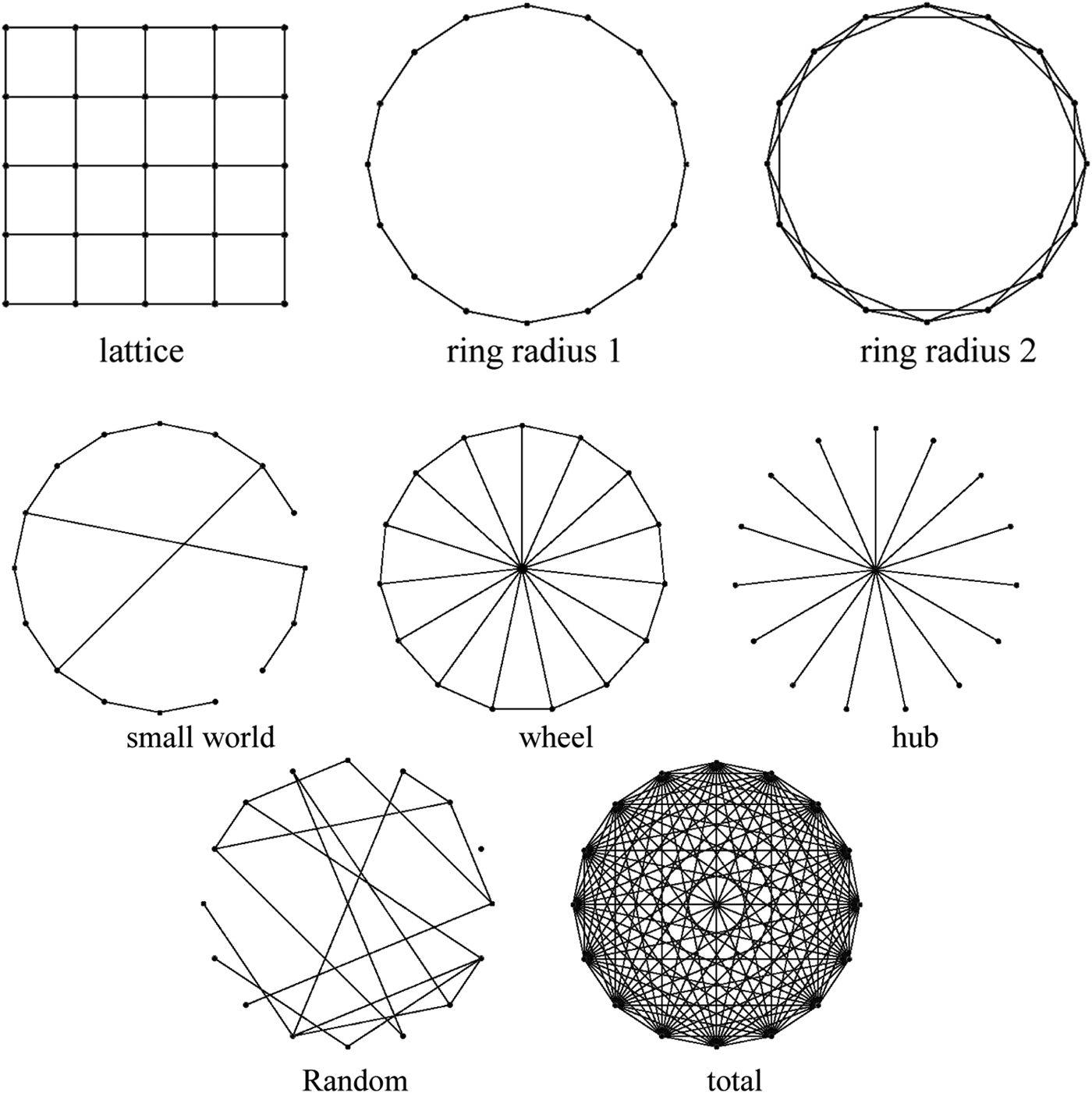
We used 50 nodes (49 in the case of the lattice) and studied the following network structures (illustrated in Fig. 6 with fewer nodes for clarity):

1. (1) a regular square lattice, with contacts to four agents on each side;

2. (2) a simple ring, with contacts to a single agent on each side;

3. (3) a ring with double radius, in which each agent has contacts with two agents on each side;

4. (4) a small world network, constructed by minimally connecting a simple ring with a 9% probability of rewiring;

5. (5) a wheel, also known as a “royal family,” in which each agent on a simple ring also has contact with a central agent;

6. (6) a hub, in which agents have contact only through a central agent;

7. (7) a random connected network with a 9% probability of combination between any two nodes;

8. (8) a total or complete network, in which all nodes are linked to all others.

To explore the effect of network structure on epistemic success, we performed 1000 runs for each network type on landscapes of increasing fiendishness index produced by the formulae given above, with random initial locations of agent hypotheses (and randomized network structure in the case of small world and random networks). For each run, we simulate 100 time steps in which each agent in the network updates its hypothesis based on its feedback using the parameters noted above for speed and margin of error.

Fig. 6.

Types of epistemic network structures. Simulations used a population of 50 nodes (49 in the case of the lattice, which wraps around).

Results for these networks on a landscape of the structure of Fig. 3 are shown in Fig. 7. The x-axis indicates the fiendishness exponent between 0.5 and 10. The y-axis reports epistemic success, that percentage of runs for a particular network in which any agent of the network established a hypothesis scoring above 0.85 (i.e., within the region of the global maximum spike above any level possible in the hump).

Fig. 7.

(colour online) Epistemic success – percentage of runs in which the spike region is found – across a range of fiendishness exponents and for a variety of networks. Spike center is located at x = 0.4.

Here, the simple ring and small world networks prove most successful across the entire range of landscape fiendishness. Random, hub, double-radius ring, wheel, and lattice networks form a middle group in terms of success, with fully connected networks the clear loser across the entire range. As the problems become more difficult to solve – for high fiendishness – the difference between networks narrows. With a fiendishness exponent of 2, probability differences are dramatic: ring and small world networks have a probability of over 70% of finding the highest peak. The middle group ranges between a probability of 42% and 58% of finding that peak. Connected networks find the peak in only a little over 20% of cases. At a fiendishness exponent of 3, the ring has a success rate of 60%. The connected network has a success rate of 18%.

It turns out, however, that landscape fiendishness and network structure are not the only factors of importance for this measure of epistemic success, even when assumptions regarding agent updating are held constant. It is not merely the existence of a hidden “needle in a haystack,” but also its position in the landscape that is of importance to these results.

In two further series we changed the landscape merely by the position of the spike. In one series, shown in Fig. 8, the spike was placed precisely in the landscape center (x = 0.5) rather than shifted to one side (at x = 0.4). With that change, the impact of network structure on epistemic success and the relative success of different networks is quite dramatic (Fig. 8).

Fig. 8.

(colour online) Epistemic success with spike located precisely in the landscape center.

Fiendishness remains the same in the two cases, since the position of the spike makes no difference to the probability of a highest random drop landing in the spike basin. Given our agent dynamics, however, position of the spike does make a difference in the success of various networks. Ring lattices and small worlds are still more successful than total networks. At a fiendishness exponent of 2, for example, ring and small world networks now have a success rate of above 95%. Total networks can boast a success rate of only a little above 25%. Ring 2 and random networks, which scored significantly below the simple ring in the earlier landscape, here track it fairly closely throughout.

In many cases the order of successful networks has changed as well. In the former landscape, with a shifted spike, the hub scored above the wheel and lattice, which were approximately equal. Here, with a central spike, the lattice is clearly superior to the wheel, which is in turn superior to the hub. A network epistemic success ordering of A > B ≈ C, in other words, has been replaced by C > B > A.

Why the difference? The answer is that our updating dynamics interact with a central landscape structure in a very particular way. With our setting for the speed parameter, approaching the hypothesis of a more successful network neighbor is in steps of 50% toward a target approximated with a margin of error of 10% of the distance. Given a landscape with a centered spike, the peaks of our sub-optimal local maxima fall precisely at 0 and 1 on the scale. If a node is on the sub-optimal hump on one side and its most successful neighbor is higher on the sub-optimal hump on the other side, our dynamics will throw him halfway toward the hypothesis of that more successful neighbor, which will tend to throw him toward the middle of the landscape, increasing the chances of hitting on a more successful hypothesis within the spike.

This result emphasizes the complexity of the phenomenon at issue. Fiendishness clearly plays a role. Network structure clearly plays a role. But precisely what role these play may depend on the interaction of agent updating and other aspects of landscape topography – in particular, the specific position of relevant peaks. This is the particular lesson of dramatic differences in results given the central spike: that not merely the proportional domain but the relative position of epistemic landscape features can spell the difference between success and failure, in some cases reversing the success dominance of particular network structures. Using a very different form of updating, in which networks do not play a pronounced role, Hegselmann and Krause (Reference Hegselmann and Krause2006) notes a similarly important role for the “position of the truth” toward the edges or in the center of an opinion space.

We don't think that the positional effect should be regarded as merely a modeling artifact. Epistemic landscapes can vary not merely in proportion of areas of success, but in the relative position of those areas to one another. A successful result may prove easier to find if it is one that is bound to be traversed in the switch from one hypothesis to another. A particular hypothesis may be difficult to hit on not merely because it is a needle in a haystack, but because that needle is located at a particularly unpropitious spot in the haystack as a whole.

The lesson we draw is that there is an additional aspect of landscapes to keep track of, and it is certainly of interest to track the relative impact of those different aspects. We also investigated the positional effects by filtering out the effect of the position of the spike by reconstructing our landscape so that it has no spatial structure bound between 0 and 1; i.e., we made it “wrap around,” thus leaving no center for a spike to occupy. With that change, we're able to extract those network effects that function independently of the positional effect.

The results for a wrap-around landscape of this type are shown in Fig. 9, zooming in to focus on the fiendishness exponent from 0.5 to 5.0 in Fig. 10.

Fig. 9.

(colour online) Epistemic success for a wraparound landscape.

Fig. 10.

(colour online) Epistemic success for a wraparound landscape, focus on fiendishness exponents from 0.5 to 5.

Figures 9 and 10 make it clear that results in the other two cases do rely on positional effects. In the case of a wraparound landscape, the divergence of successful from unsuccessful strategies is far less, though at many points the most successful strategies – ring and small world – still have a success rate almost twice that of total networks. At a fiendishness exponent of 1, ring and small world arrays have a success rate of approximately 80%; total networks come in at only 48%. At a fiendishness exponent of 1.5, ring and small world networks approximate a 60% success rate, while total networks are at approximately 32%. In the wraparound landscapes, the order of relative success is the same as our original graph, though the field gets crowded above a fiendish exponent of 4.5 or so.

Interestingly, the case can be made that lattices share the bottom of the pecking order here, precisely as they occupied part of the top region in the case of a central spike. This seems all the more significant since so much work has been done using square lattices (e.g., on cooperation, segregation, and the emergence of language) as if the results were generalizable to networks more broadly (Schelling Reference Schelling1969, Reference Schelling1978; Axelrod Reference Axelrod1984; Boccara et al. Reference Boccara, Goles, Martinez and Picco1993; Hegselman and Flache Reference Hegselmann and Flache1998; Cangelosi and Parisi Reference Cangelosi and Parisi2002; Grim et al. Reference Grim, Selinger, Braynen, Rosenberger, Au, Louie and Connolly2005, Reference Grim, Wardach and Beltrami2006; Grim Reference Grim2007). The same worry applies to Weisberg and Muldoon (Reference Weisberg and Muldoon2009) as we mentioned above.

The above results use a particular set of assumptions regarding agent updating to offer a more precise picture of the differential impact of investigatory networks over increasing question difficulty. In doing so, the important and unexpected role of what we have termed “positional effects” was highlighted.

5. ANOTHER SCIENTIFIC GOAL: CONVERGENCE

The scientific community puts significant weight on individual discovery – the element of epistemic success we focused on in the last section. But science could not proceed if a discovery remained solely with the discoverer. Dissemination of discoveries allows other scientists to rely on those discoveries and further their own work, and it allows non-scientists to use that information in policy-making and education. The desiderata of both dissemination and discovery are reflected in standard rules governing scientific priority: that the glory goes to the first presentation or publication of a discovery.

The dynamics of the current model guarantee that consensus will emerge since agents always move their hypotheses toward that of more successful neighbors. The amount of time required for convergence of opinion to occur, however, may depend on both the communication network and the epistemic landscape. Kevin Zollman has repeatedly called attention to the trade-off between scientific goals of accuracy and speed (Zollman Reference Zollman2007, Reference Zollman2010a, Reference Zollman2010b, Reference Zollman2012). Here we can outline some details of that trade-off against a background of epistemic landscapes with varying degrees of fiendishness.

Recall from above that the ring network is generally the best communication network in finding the hidden spike of a fiendish problem. But as Figs 11 and 12 show, for both the bounded and offset and wraparound landscapes, it is also the ring network in which consensus takes the longest time to achieve.

Fig. 11.

(colour online) Time to convergence for a bounded and offset landscape (peak at x = 0.4).

Fig. 12.

(colour online) Time to convergence in a wraparound landscape.

If the goal is fast consensus, total networks are clearly optimal. But total networks also do the worst in terms of accuracy. Roughly and qualitatively, the time to consensus and the percentage of runs that find the spike share close to the same ranking: those distributed networks in which exploration is relatively insulated against immediate input from the group are those which have the highest rate of success in individual discovery but also take the longest to achieve a consensus of recognition and adoption.

The precise time to consensus for a given network differs between bounded and offset and wraparound landscapes, just as does the precise percentage of runs in which it finds the highest peak. What holds for both landscapes is the general inverse ordering between accuracy and time to consensus. The higher a network's accuracy on either landscape, the slower its time to consensus. We should therefore expect a bounded landscape with a centered spike, which shows the highest success rates, to show the longest times to network consensus as well. This is indeed what the data show (Fig. 13).

Fig. 13.

(colour online) Time to convergence with a central spike.

There is an obvious difference between these graphs. Beyond a fiendishness exponent of 2 or so there is a quick decline in time to convergence in the case of both the wraparound and bounded and offset landscapes, while time to convergence in the case of the central spike shows something closer to a plateau. The declines in Figs 11 and 12 occur because decreasing success, i.e., convergence on the highest point in the landscape, is accompanied by the increasing speed of convergence on the suboptimal hump. If we map instead time to convergence limited to those cases in which convergence was on the highest, we see the appropriate increase in time with increasing question difficulty (Figs 14 through 16). Within those constraints, we see that the convergence results are remarkably uniform.

Fig. 14.

(colour online) Time to convergence on a bounded and offset landscape among cases in which convergence is on the highest peak.

Fig. 15.

(colour online) Time to convergence on a wraparound landscape among cases in which convergence is on the highest peak.

Fig. 16.

(colour online) Time to convergence on a bounded and centered landscape among cases in which convergence is on the highest peak.

6. EPISTEMIC SUCCESS AND CONVERGENCE ON THE WATTS–STROGATZ CONTINUUM

In the previous two sections, we analyzed the impact of network structure on epistemic success (measured in terms of whether any agent finds the peak) and time to convergence. Following Zollman (Reference Zollman2007), our method has been to focus on a handful of representative network structures to tease out which aspects of network structure are influenced on the target phenomena. Here we introduce a new technique, that of analyzing data produced by a series of models that contain networks produced by systematically varying a network structure parameter.

In the data above, it appears that that median node degree roughly tracks the observed results. The highest achieving networks in terms of accuracy are consistently those with the lowest degree; the worst performing is the total, with the highest degree. Those networks which are slowest to achieve consensus are those with the lowest degree; those with high degree converge quickly for precisely that reason.Footnote ²

But neither epistemic success nor convergence are purely a matter of degree. Within the limits of keeping rewired networks connected, our ring and small world networks have the same mean degree, track each other closely in terms of success, but diverge importantly in terms of speed to consensus. The 4-lattice and the radius-2 ring networks (in which each node is connected to two neighbors on each side) are both regular networks with a uniform degree of 4. But both success and convergence rates differ significantly between them.

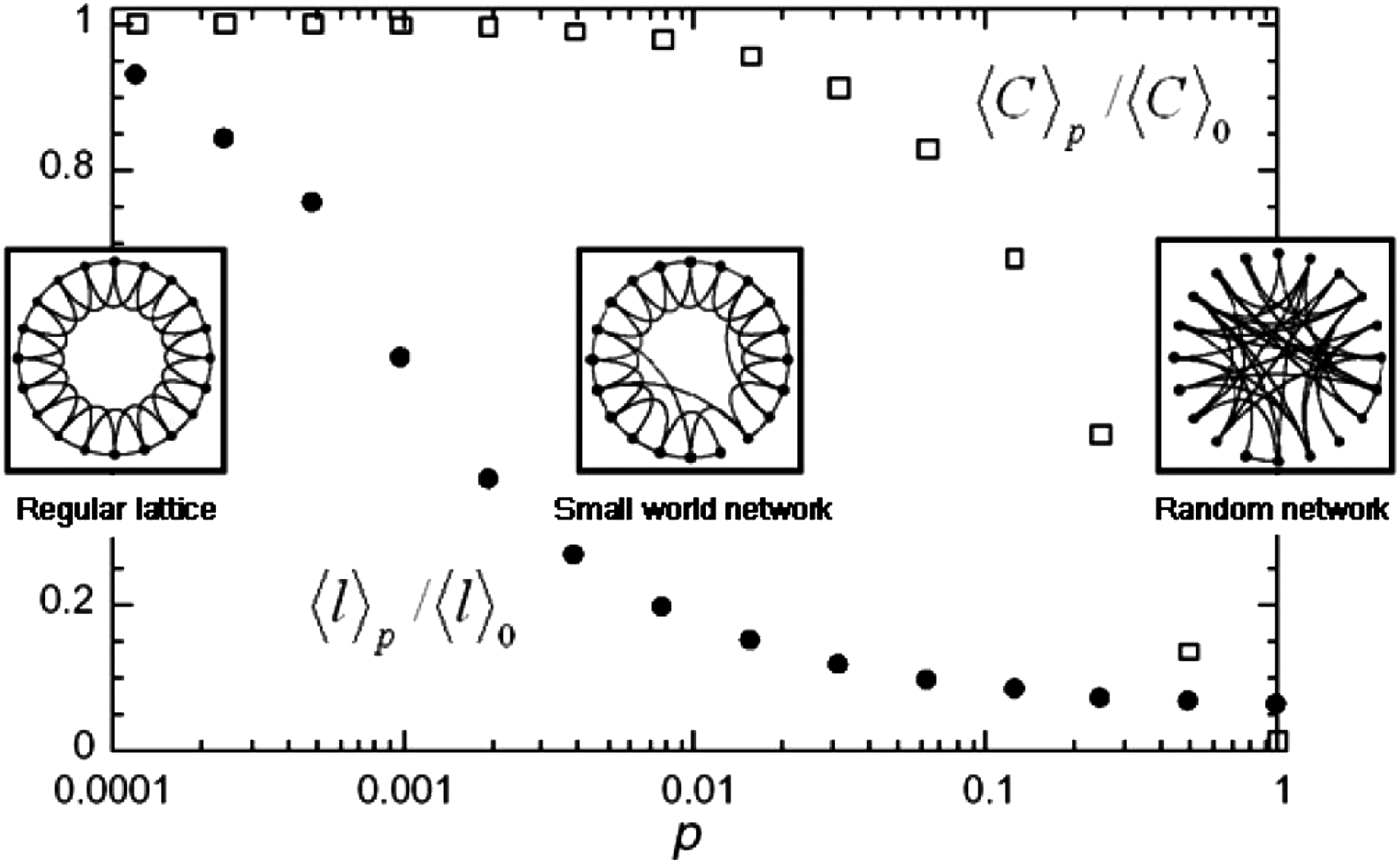
In order to get a better feel for relevant network properties we lay out patterns of epistemic success and convergence in comparison with the well-known Watts–Strogatz model, which produces a series of small-world networks by varying a rewiring parameter. Watts and Strogatz (Reference Watts and Strogatz1998) start with a ring of 1000 nodes, each connected to the 5 nearest on each side. The series of networks is produced by increasing the probability that any link will be rewired randomly, until it reaches 1, where the network is completely random. Across that scale, Watts and Strogatz measure both clustering coefficient – the proportion of node pairs connected to a focal node that are also connected to each other – and characteristic path length – the average number of steps along the shortest paths among all pairs of nodes. When laid out on a log scale, the measure of clustering coefficient across that continuum of increasingly random networks shows an importantly different pattern than does mean path length.

Clustering coefficient and path length are both normalized to their highest value. Watts and Strogatz present their result in terms of a mean of 20 runs. That actually makes the data appear somewhat cleaner than they actually are. The original illustration from Watts and Strogatz appears in Fig. 17.

Fig. 17.

Normalized clustering coefficient and characteristic path length across increasing probabilities of near-neighbor link rewiring (Watts and Strogatz Reference Watts and Strogatz1998).

Figure 18 shows our replication of the Watts–Strogatz runs, using probabilities from .0001 and marking values for each of the 20 runs. It is clear that mean path length across the spectrum has a significantly wider variance than one might have expected from its original presentation.

Fig. 18.

(colour online) Replication of the Watts–Strogatz runs, showing the variance in mean shortest path length.

Using our replication of the Watts–Strogatz series of networks, we ask whether epistemic success tracks characteristic path length or clustering coefficient. Duplicating Watts and Strogatz's 1000 node networks against a fiendishness exponent of 2.5 for all of our landscapes, it turns out that epistemic success follows neither one.

Across that continuum of networks, the percentage of runs in which the highest peak is found is over 90% in all cases, demonstrating no pattern that suggests that either shortest path length or clustering coefficient closely tracks it. So, for epistemic success, something other than these simple network measures must be at work. Figure 19 shows results for a bounded landscape in which the spike is offset from the center. Figure 20 shows epistemic success for a wraparound landscape. In the case of a bounded and centered landscape, all networks across the continuum had a success rate of 100%. Here the results are shown for the mean of 100 runs in all cases except the bounded and offset network, in which results are shown for the mean of 1000 runs.

Fig. 19.

(colour online) Epistemic success across the Watts–Strogatz spectrum of networks, using a bounded and offset landscape with a fiendishness exponent of 2.5.

Fig. 20.

(colour online) Epistemic success across the Watts–Strogatz spectrum of networks, using a wraparound landscape with a fiendishness exponent of 2.5.

When we turn to the amount of time it takes for the network to converge on a hypothesis, the story is very different. Here the behavior of our epistemic networks does follow a simple network property – that of characteristic path length. Figures 21 through 23 show superposition of time to convergence over the characteristic path length obtained in our replication of Watts and Strogatz above.

Fig. 21.

(colour online) Time to convergence across the Watts–Strogatz spectrum, using a bounded and offset landscape.

Fig. 22.

(colour online) Time to convergence across the Watts–Strogatz spectrum, using a wraparound landscape.

Times to convergence on both the bounded and offset and wraparound landscapes lie squarely along the values for mean shortest path length. Although the curve is the same in a bounded and centered landscape (Fig. 23), the pattern is somewhat different in that case: it is intriguing to note there that time to convergence in that case is slower through the region of small worlds than one would expect from shortest path length alone.

Fig. 23.

(colour online) Time to convergence across the Watts–Strogatz spectrum, using a centered spike landscape.

Above, we noted the inverse orderings of successful as opposed to quickly converging networks among our samples, which is consistent with the lesson from Zollman (Reference Zollman2007, Reference Zollman2010a). But despite that inverse ordering, the fact that time to consensus tracks characteristic path length in the network, while epistemic success does not, indicates that there are different aspects of network structure at work in the two phenomena. Time to convergence parallels shortest path length quite closely. Epistemic success, even in the simple model we have outlined here, turns out to be significantly more complicated across both our networks and those in the Watts–Strogatz series of networks.