1. Introduction
Given a probabilistic causal model that describes the causal structure for many possible situations, how does one assign credit or blame for what actually happens? Causal models have a natural semantics: variable C is a cause if and only if (iff) there is some context in which a change in the value of C would make a difference to E (see, e.g., Woodward Reference Woodward2005). But in actual causation, we do not care that “there is some context.” We want an answer for this actual context. Certainly smoking can kill, but did Jones's smoking kill him?
In Handfield et al. (Reference Handfield, Twardy, Korb and Oppy2008), we argued for integrating causal models with process-theory semantics. Here we attempt to push stochastic causal models as far as they can go alone. Although finally incomplete, the account can surpass the limits declared by Hiddleston and others. We demonstrate the model on several problematic examples from the literature, including cases of overdetermination and “late cutting” (where a slower potential cause is rendered otiose by a faster-acting cause).
This article extends “active path” accounts such as those of Hitchcock (Reference Hitchcock2001) and Halpern and Pearl (Reference Halpern and Pearl2005a, Reference Halpern and Pearl2005b). The key idea is that in a given context, some paths become inactive. An actual cause must be on an active path. But earlier accounts assume deterministic networks, which is unnecessary and contrary to the spirit of probabilistic causal models. Determinism also masks some subtleties, much as using binary variables can mask intransitivity.
2. Deterministic Active Paths
Following Hiddleston (Reference Hiddleston2005), we use H1 for Hitchcock's “strongly active path,” H2 for Hitchcock's (Reference Hitchcock2001) “weakly active path” with redundancy ranges, and H3 for Halpern and Pearl (Reference Halpern and Pearl2005a, Reference Halpern and Pearl2005b). We will present a reconstruction that blends H2 and H3.
2.1. Strongly Active Paths (H1)
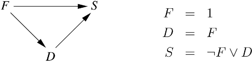
A boulder falls (F) toward a hiker (Hitchcock Reference Hitchcock2001). The hiker sees the boulder in time, and ducks (D), thereby surviving (S). Each variable is binary. We represent the causal variables as nodes in a graph and the causal links as arrows between them. We specify the exact dependencies with a series of simple structural equations, as in figure 1. The first equation gives an initial condition: in the actual world, the boulder falls. The second says that the hiker ducks if the boulder falls. The third says the hiker survives if he ducks or if the boulder does not fall. The causal model is fully specified by the equations and the possible values for each variable.
Boulder example. D = ducks; F = falls; S = survives.

Causal models specify the counterfactuals over the variables in the model, in the same way a circuit diagram specifies the effect of any alteration or failure of its components (Pearl Reference Twardy and Korb2000). Counterfactuals do not backtrack. If they did, ducking would make no difference to survival. But counterfactuals are assessed by interventions, not observations. We do not observe that D is 1. Instead, we replace the structural equation  with
 and reevaluate. The boulder falls
 , and
 when
 , and
 when
 , so ducking makes a difference. Therefore, we want to say that ducking caused survival. Conversely, we do not want to say that the boulder falling caused survival. The difference is that only ducking has an active path to survival.
We now define active path actual causation (APAC). A path is a traversal from C to E along the arrows, in the direction of the arrows. Then:
Definition 1 (APAC).  was an actual cause of
 iff there was an active path from C to E (and actually
 and
 ).
Intuitively, a path is active if it makes a difference. A path is strongly active if c makes a difference to e when all other paths between C and E are blocked by setting variables along those paths to their actual values. “Making a difference” has the usual counterfactual meaning: had C been different, E would have been different, for at least some  .
In Boulder, neither of the paths from F to S is strongly active. First, we hold D fixed at its actual value  blocking
 and leaving only
 . But since
 , F makes no difference: given that the hiker ducked, the boulder has no effect. The path
 is not strongly active.
To evaluate  for strong activity, we would have to block
 , which we cannot, as there is no intermediate variable. With nothing to block, we are back to the original case where F makes no difference to S because the paths cancel. We happily conclude that F did not cause S. “Intuitively, the falling boulder does not save Hiker's life because without it, Hiker's life would not have been endangered in the first place” (Hitchcock Reference Hitchcock2001, 295).
When we are considering a particular path, all ancestors of E not on it constitute the background. A straightforward (if inefficient) attempt to block all but one path is to intervene to set the whole background—all ancestors of E except those along our path . Call this background β.
Definition 2 (Background β). Given a target variable E and path ending with E, the background β is all the ancestors of E except for those in .
Definition 3 (β-actual model). Given target variable E, the β-actual model replaces all the equations for β with their actual values  . The replacements are by intervention.
We can now give a formal definition of strong activity. Let  , or just
 , denote that we intervene to set
 ; similarly for
 . (We shall also use “set” as an English equivalent for the I notation.) We assume throughout that C is the beginning of the path and E its end. Then:
Definition 4 (Strongly active path). A path is strongly active iff  (vs.
 ) makes a difference to E, in the β-actual model, for some c and
 .
If we allow only strongly active paths, then APAC yields Hitchcock's first active path account, which Hiddleston (Reference Hiddleston2005) dubs H1. Unfortunately, H1 handles neither symmetric overdetermination nor late cutting. We review redundancy ranges to handle overdetermination and then resetting ranges to avoid late cutting. Afterward, we present our probabilistic reformulation.
2.2. Redundancy Ranges
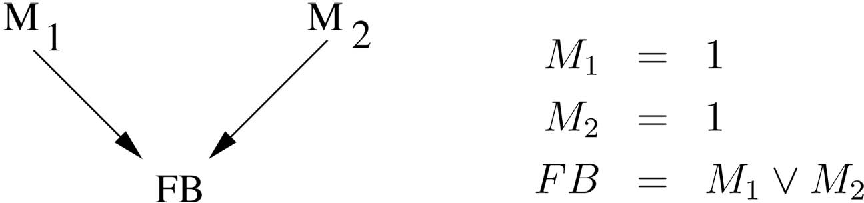
Symmetric overdetermination happens, given multiple sufficient causes. One such case is Matches. Two lit matches (M 1 and M 2) are dropped in the forest. Either would suffice to burn it down, and the forest burns down (FB; fig. 2).
Matches example. FB = forest burns; M = match.

The reader can verify that neither match has a strongly active path. However, intuitively both matches contributed to the fire, although neither alone was necessary. The causal structure allows us to reveal the hidden dependency.
Note, we can let M 2 be 0 without affecting the result—the forest still burns down. Hitchcock calls the set of such “redundant” settings of background variables the redundancy range.
Definition 5 (Redundancy range). Given a particular path and background β,  lies in β's redundancy range for E iff
 leaves E unchanged.
The redundancy range is the set of all possible ways of fixing the background variables so that they make no difference to E. Of course, the actual values of β are also in the redundancy range.
Definition 6 (β model). The  model replaces all
 with values
 in their redundancy range, via
 .
In Matches, by setting  , we reveal a hidden dependency: now
 makes a difference. We define an active path (simpliciter) as a path that becomes strongly active when we set background variables to some values in their redundancy range (H2).
Definition 7 (Active path). A path is active iff  (vs.
 ) makes a difference to E in some
 model. More precisely,
 gives e and
 gives
 .
Both paths in Matches are active, so both matches are causes according to definition 1. But we cannot yet handle late cutting.
2.3. Resetting Ranges (∼H3)
Late cutting is a kind of preemptive overdetermination. It occurs when one of the potential causes preempts the other, precisely by completing first. For example, Bottle:
Suzy and Billy throw rocks at a bottle. Suzy's rock arrives first, breaking the bottle before Billy's rock, which would also have broken it.
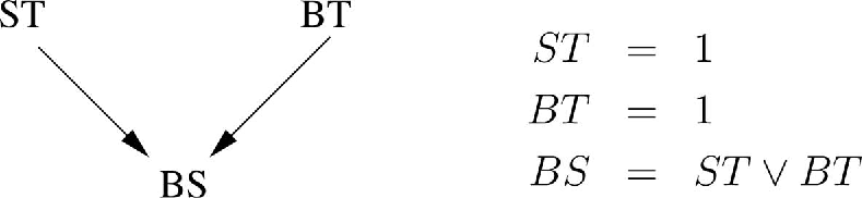
We want to say that Suzy's throw (ST) caused the bottle to break (BS) but that Billy's throw (BT) did not. First, note that the obvious model (fig. 3) does not work. This is the same model as Matches, so it gives the same answer: both throws caused the bottle to smash. But our intuitions strongly favor Suzy's throw over Billy's: the preemption matters.
Bottle example. BS = bottle shatters; BT = Billy throws; ST = Suzy throws.

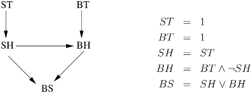
Halpern and Pearl (Reference Halpern and Pearl2005a) argue that this model misrepresents the case since the model is symmetric and Bottle is not. They argue that a proper model should show the key asymmetry: when Suzy's throw hits (SH), it prevents Billy's from hitting (BH). Therefore, Halpern and Pearl suggest the model in figure 4.
Modified bottle example. BH = Billy hits; BS = bottle shatters; BT = Billy throws; SH = Suzy hits; ST = Suzy throws.

This seems a good model, and it works for Suzy, whose path is strongly active. Unfortunately, Billy's path  is also active. Let
 :
 is in the redundancy range, and under
 , BT makes a difference.
Hitchcock's H2 solves that problem by requiring that  not change anything on the path , whereas
 implies a change to BH. But Halpern and Pearl showed that this strategy was vulnerable to a voting machine example (Twardy and Korb Reference Twardy and Korb2011). Their solution is to allow resetting of variables along . We now present a somewhat simplified version of resetting variables.
Definition 8 (H3AP). is active iff:
A. When we set
 and as in definition 7, we get .
B. When we set c and
, we get e, even if we reset any of the other variables in to their actual values.
 and
 as in definition 7, we get
 .
 , we get e, even if we reset any of the other variables in to their actual values.
Note that resetting is only done for  ; otherwise, no cause could make a difference.
Condition A amounts to saying that there is a background state  where c can make a difference to e. Condition B ensures that the background
 alone is insufficient to force
 : it means that
 is in the redundancy range for e. The “even if” clause about resetting variables in to their actual values is only necessary in cases of late cutting.
In the extended bottle-smashing model, Suzy's throw  remains an actual cause of
 using a redundancy range to reveal the dependency. Choosing
 as our background, and setting
 , we see that ST makes a difference. Resetting has no effect because, actually,
 .
Billy's throw would similarly make a difference, save for the new “resetting” clause. Let the background be  . Setting
 , Billy's throw makes a difference. However, we can reset BH to its original value when
 . Of course, then Billy's throw will no longer make a difference, and
 , in violation of clause B of definition H3AP. Therefore, this path is not an active path, and BT is not an actual cause. We turn now to probabilistic extensions.
3. Probabilistic Active Paths
The counterfactuals in H1–H3 are of the form, “if not  , then not
 .” That will not work for probabilistic causation. In Matches, if each match acts independently with probability p of burning down the forest, then both matches will have a greater probability of burning down the forest, but it still might not burn down. Conversely, the model could allow the forest to burn down with neither match lit: active paths need to be redefined in terms of changing probabilities rather than changing states. Except for noting that by “cause” we will henceforth mean “causally relevant,” we retain APAC. (We can distinguish promoters from preventers by examining whether the probability went up or down.)
We will use two measures of probabilistic difference making. The first measure,  , is the difference caused by c in some background
 .

Intuitively, a path is active when  . However, with finite data to estimate probabilities and limited computing power, we cannot be so stringent, so we introduce a tolerance parameter. Let ε denote some threshold below which we consider changes in probability to be insignificant. Then, a path is active when
 . (If
 , then the path is an active preventer.)
To be strongly active, we must have  in the β-actual model, when
 . But in general,
 can be any member of the redundancy range, which are instantiations of β whose effect on
 is less than ε.
We define  to be the effect of wiggling
 versus
 in “background” c:

Instantiation  lies in β's redundancy range iff
 . This already is sufficient for handling probabilistic matches (see fig. 5).
Probabilistic matches example. FB = forest burns; M = match.

Let s and t be the probabilities that  and
 , respectively, acting alone would burn down the forest (i.e., in this case
 ). The model combines these probabilities independently in determining the probability of FB (i.e., there is no “synergy” between the two causes). The model also assumes the forest cannot burn down spontaneously (or, indeed, by any other cause than the matches named); this is recorded in the third equation, where the exponents just switch the terms on and off. That equation expresses the idea that
 and
 act independently since their chances of failure simply multiply.
Variables  and
 are only strongly active (i.e., active relative to the other match being lit) for
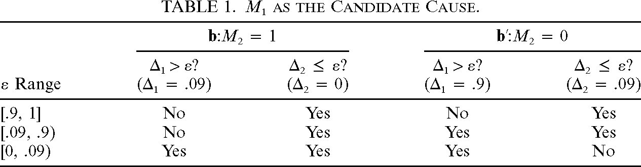
 . We can construct table 1, relative to
 as the candidate cause. There are two cases when
 is counted as a cause, depending on ε. If
 , then
 is a cause because its path is active in the actual case
 . If
 , then
 is a cause because its path is active in the redundant case
 . If
 , then
 is not a cause. The analysis is symmetrical for
 . Therefore, if
 , both matches cause the forest to burn down, but if
 —a very large tolerance—then neither does.

 |
 |
|||
 ? |
 ? |
 ? |
 ? |
|
| ε Range | ( ) |
( ) |
( ) |
( ) |
| [.9, 1] | No | Yes | No | Yes |
| [.09, .9) | No | Yes | Yes | Yes |
| [0, .09) | Yes | Yes | Yes | No |
We can make the model “feel” more deterministic by defining  . In that case,
 so long as any match is lit. Clearly, neither is strongly active for any ε. Nevertheless, both are active simpliciter for any
 . Setting
 recovers the original deterministic Matches exactly, concluding that both matches are actual causes (so long as
 ); the same, of course, can be said of the original model.
3.1. Soft Interventions
The final step will be to introduce resetting ranges, dealing with late cutting. However, for assessing active paths probabilistically, we turn to “soft interventions.” A soft intervention (Korb et al. Reference Korb, Hope, Nicholson, Axnick, Zhang and Güsgen2004) fixes a variable to a distribution, instead of a single value. For example, fixing  (i.e., a 70% chance of Suzy hitting) is a soft intervention. The proper probabilistic analog of “setting X back to the value it would have under c” is “setting X back to the distribution it would have under c.”
Soft interventions are easily dealt with formally. A soft intervention on X is implemented by adding a new parent  , such that when I is true,
 takes the desired distribution, and when I is false, X has its previous distribution. How this might be done experimentally (outside of simulation) is less clear. Nevertheless, many actual interventions are soft rather than hard (Korb et al. Reference Korb, Hope, Nicholson, Axnick, Zhang and Güsgen2004). In any case, we are not here concerned with implementation but with using soft interventions as a calculating tool.
The soft interventions of interest here freeze X at its current distribution. Because the distribution is unchanged, such interventions have no downstream effect. However, all back paths are severed: changes in parent values (other than I) have no effect on X; changes in X can only then tell us about I and not its other parents or, through them, any cousin variables. This gives us exactly what we need: the ability to distinguish causes and effects by the asymmetries of intervention. In this article, we denote such distributional (soft) interventions with a vector symbol  —or
 —denoting that we have simply replaced the distribution for C. (When we do not specify that new distribution, by default we shall mean the current distribution.)
3.2. Resetting Ranges and Probabilistic Active Paths
Let there be n variables along path , not counting C and E. There are  possible combinations for clamping (or not). Let
 denote the set of possible “resetting ranges,” the power set listing all possible combinations of these variables. Then for
 , let
 denote the intervention resetting those variables in
 to their current distribution. We can now define the probabilistic active paths (PAP) criterion:
Definition 9 (PAP). A path is active iff for some background  :
1.
. (Wiggling C makes a difference.)2.
. (Wiggling alone does not make a difference.)3. In
, leaves , .
 . (Wiggling C makes a difference.)
 . (Wiggling
 alone does not make a difference.)
 ,
 leaves
 ,
 .
Condition 3 requires that condition 2 holds for all combinations of variables in ; that is, resetting them to their original distributions leaves  in the redundancy range. As noted, we add our clamp
 to the interventions already done for
 . A brute force search over the power set of resetting ranges will naturally be expensive, but we are not concerned with that here. For the small models treated in this literature, the problem is not serious.
4. Probabilistic Examples
Here we review the application of PAP to some examples from the literature. PAP deals well with deterministic examples (if H3 does) because PAP with degenerate distributions is H3. So here we treat only probabilistic variants of the examples.
4.1. Probabilistic Bottle
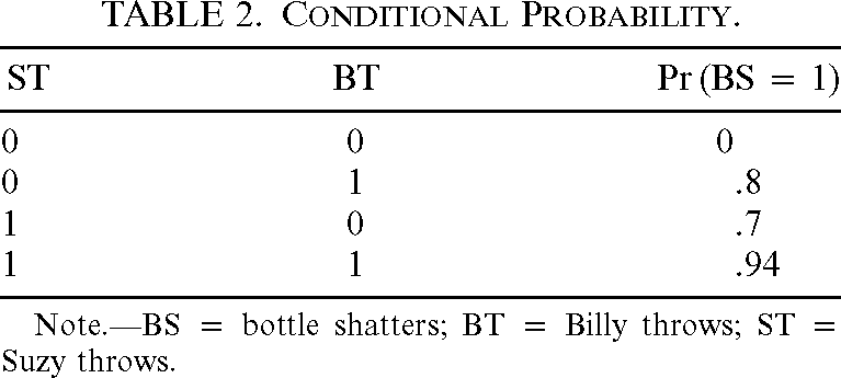
For a more realistic version of Bottle, we allow that Suzy and Billy sometimes miss. In particular, given knowledge only of ST and BT, we use table 2. We use the extended model of Halpern and Pearl to capture the timing asymmetry as before, yielding figure 6.

| ST | BT |  |
| 0 | 0 | 0 |
| 0 | 1 | .8 |
| 1 | 0 | .7 |
| 1 | 1 | .94 |
Note BS = bottle shatters; BT = Billy throws; ST = Suzy throws.
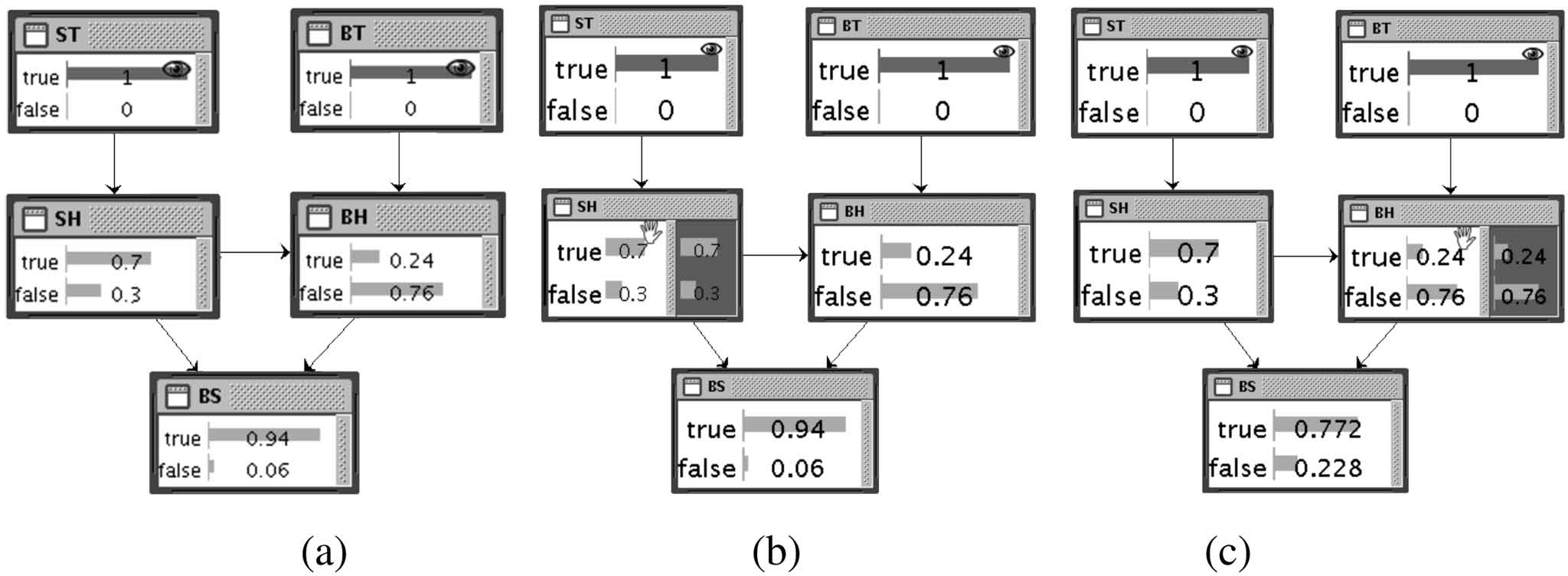
Probabilistic version of bottle with results of intervening to fix the probability distributions: a, original state; b, clamping SH has no effect on BS; c, clamping BH affects BS. BH = Billy hits; BS = bottle shatters; BT = Billy throws; SH = Suzy hits; ST = Suzy throws.

Let  , so the redundancy ranges are degenerate for both Suzy and Billy: we have to use the actual background
 or
 . The network is shown in three states in figure 6. The original distribution is in figure 6a. As before,
 and
 for both Suzy and Billy. Next, we see whether resetting the intermediate “hits” variables violates condition 3.
In figure 6b, we consider Suzy, resetting to  . This leaves
 unchanged, so we conclude that Suzy Throws is an actual cause. In figure 6c, we consider Billy. Resetting to
 ,
 changes, so
 , and BT is not actually a cause on PAP. This happens because the intervention on BH blocks the backward flow of probability otherwise relating BS and BH through their common cause SH. Before resetting, the distribution
 arose because Billy could hit only when Suzy did not. Suzy missed 30% of the time, and
 . Now, however, Billy never hits more than 24% of the time, so
 drops from 94% to 77%.
The original probabilistic Boulder can be resolved without resetting. However, if we add noise at S, so that ducking no longer guarantees survival, we find an influence for F, which we argue is appropriate. (For further analysis, see Twardy and Korb Reference Twardy and Korb2011, the online companion piece.)
4.2. The Trainee Assassin
The deterministic version is that a trainee assassin T shoots a victim V, but Supervisor will shoot if Trainee loses nerve. Being deterministic, Victim survives only when neither shot is fired. In the actual case, the trainee shoots, the supervisor does not, and the victim dies. As with Boulder, there is no marginal effect, but any path-based account works because the path  is strongly active. However, Hiddleston (Reference Hiddleston2005) alleges that the analysis will not survive a probabilistic extension, which leads us to the stochastic assassin.
4.3. The Stochastic Assassin
In the probabilistic version, Trainee firing lowers the overall chance that Victim dies, by preventing the more accurate Supervisor from shooting. Once again, a path-based analysis of actual causation does fine here. Let  and
 . For completeness,
 .
Since Supervisor does not shoot, Trainee is strongly active with  . Similarly, Supervisor's
 (vs.
 ) has
 in the actual background where Trainee shoots, and so is a strongly active preventer (of death), having the same status as the falling boulder. That is, Supervisor is ineluctably causally active.
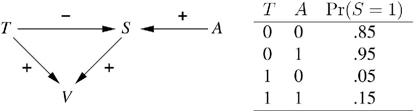
Hiddleston recommends adding an extra variable for Supervisor taking Aim (A). The supervisor is unlikely to fire without aiming and is always more likely to fire if she aims. Avoiding extremes, let Supervisor be 90% likely to fire if Trainee loses nerve and 10% likely even if Trainee also fires. Let those numbers average over Aiming and not-Aiming, with a 5050 prior over each. Furthermore, let aiming improve chances 10% over not aiming in both cases. The model and conditional probability table are shown in figure 7.
Stochastic assassin example, with supervisor's conditional probability table. A = aiming; S = supervisor; T = trainee; V = victim.

As before, let T and S be independent causes of V (in a noisy-or model). Consider whether  is an actual cause of
 . In the actual background,
 , and
 . Aiming appears to be an actual cause, provided
 . Clamping S at the distribution
 induced by
 has no effect on
 . Therefore,
 is on an active path and is a cause.
Hiddleston thinks this is wrong because in actual fact Supervisor did not shoot, so Aiming made no difference. We disagree. As our analysis has made clear, when considering the probabilistic effect of C on E, one must unfix the path between C and E. If we fixed S, we would cut the active path and get Hiddleston's answer, but in a probabilistic context that procedure implies that only direct causes are actual causes. Hiddleston is correct that such probabilistic accounts cannot work, but that is just a misconstrual of probabilistic accounts. Hiddleston's superfluous antidote presents more of a problem.
4.4. Superfluous Antidote
Fred injects himself with a harmless antidote  in the false belief that he has been (or is about to be) poisoned (P). The model is simple:
 , and
 . Fred survives when
 . In fact there is no poison
 , so the antidote is irrelevant. However, because
 , the redundancy range includes
 . Were there poison, the antidote would make a difference; hence, the path
 is active. As Hiddleston says, “That is the wrong answer. H2 [and H3] counts
 an ‘actual cause’ merely because it would have been a cause if the circumstances had been different” (Reference Hiddleston2005, 32).
This is a good counterexample because it targets redundancy ranges, an epicycle added to handle symmetric cases. H1, which lacks redundancy ranges, correctly says  is not a cause. But it also says
 is not a cause, leaving
 uncaused, as it does with Matches. Several responses might mitigate the damage:
• Pick one's poison, trading off cases like Matches for those like Superfluous Antidote. This is unsatisfactory since nothing is mitigated.
• Make the problem probabilistic. For many reasonable values of ε,
in the actual background , or if we try to set . That solves the problem. However, the point of the example involves extreme probabilities, which this response ignores.• Hiddleston recommends employing Cheng's account of causal power (Cheng Reference Cheng1997).
• Argue that the model structure is wrong. Hitchcock (at PSA 2010) noted that antidote and poison have to mix in the body; if we represent that aggregating variable, the problem disappears. While solving the problem, we should like an independent account of when a model is adequate. Handfield et al. (Reference Handfield, Twardy, Korb and Oppy2008) and Korb and Nicholson (Reference Korb, Nicholson, Holmes and Jain2008) sketch an account using the idea of “possible processes.”
 in the actual background
 , or
 if we try to set
 . That solves the problem. However, the point of the example involves extreme probabilities, which this response ignores.
We think that some combination of the last two responses—a mixture of an analysis of causal strength with a metaphysical analysis of causal processes—is the most promising framework for completing the story of actual causation.
5. Conclusion
Active path approaches treat actual causation in the same way one might treat type causation—assessing causal relevance by wiggling a potential cause and reading the changes in a downstream variable—except in applying a restricted context. The trick is to find the right context to do justice to our intuitions.
Hitchcock (Reference Hitchcock2001) and Halpern and Pearl (Reference Halpern and Pearl2005a, Reference Halpern and Pearl2005b) made some progress in this using deterministic criteria, that is, using only the Bayesian network structure and ignoring parameters. We have addressed that limitation, extending active path analyses to probabilistic models and defending the project against impossibility claims. Nevertheless, the resultant analysis is incomplete. For example, it cannot independently handle Hiddleston's superfluous antidote case. For such cases, we suggest considering an account that unifies difference making with causal process metaphysics, such as that presented in Handfield et al. (Reference Handfield, Twardy, Korb and Oppy2008).