


1. Introduction
Nature-based carbon capture enhances the ability of forests, soil and water to absorb CO2. Given the challenges of fully decarbonising certain economic sectors and the urgency of reducing atmospheric carbon and global emissions, carbon capture is increasingly regarded as an essential instrument in climate policy. Developing countries significantly contribute to nature-based carbon capture because they host most of the world’s natural carbon sinks, including tropical forests, peatlands and water reservoirs. Setting the right price for these carbon capture natural sources is crucial for integrating developing countries into effective and equitable climate policy.
This paper develops a macroeconomic framework for optimal carbon markets. In the model, energy use in production generates emissions that accumulate in the atmosphere and cause economic damages in the form of output losses – a climate externality. Two mechanisms offset emissions: a costly technological process and natural carbon sinks that capture carbon when individuals undertake preservation efforts. The socially optimal outcome accounts for both the social cost of emissions and the social value of carbon capture. In a market economy, a carbon price ensures that individuals and firms internalise these costs and benefits – a standard Pigouvian approach Pigou (Reference Pigou1920).
The central result of this paper shows that a carbon tax alone is sufficient to implement the socially optimal allocation. This means that a carbon tax effectively implements a carbon market, where emissions are taxed, and carbon capture has a market value. Carbon capture is valuable because it directly absorbs atmospheric carbon – the source of the climate externality. Additionally, firms that cannot reduce emissions quickly enough can offset them through carbon capture, lowering their tax bill. Importantly, the value of carbon sink preservation is internalised through the market. When a carbon price exists, carbon sinks immediately become assets that generate a positive return equal to the carbon price.
A key implication of this result is that it challenges the traditional concept of ‘additionality’, which defines the value of carbon capture based on whether it would not have occurred without policy intervention. Under the additionality criterion, only carbon sequestration that depends on policy incentives qualifies for compensation. For example, this approach would leave the carbon absorbed by the Amazon rainforest unpriced unless there were an imminent and verifiable deforestation threat. However, an optimal carbon pricing system does not follow this criterion. Instead, it assigns value to all carbon capture, ensuring that every unit of sequestration receives appropriate compensation. The optimal carbon price accounts for both positive and negative emissions, creating a comprehensive and efficient incentive structure.
Additionality arises in voluntary carbon markets precisely because there is no market price for carbon emissions. Without a price for emissions entering and leaving the atmosphere, additionality assumes that positive emissions will persist and assigns a price only to extra efforts to absorb them. Imposing – or not imposing – an additionality criterion is particularly relevant for nature-based carbon capture. Technological carbon capture inherently qualifies as additional because firms would not invest in it without a price mechanism to incentivise investment. In contrast, natural carbon sinks already exist, providing global and local benefits that remain unpriced – leading to their overexploitation. However, once emissions have a market price, expecting natural carbon sinks to provide carbon sequestration for free while placing a cost on emissions becomes difficult to justify.
A secondary result of the paper shows that additionality arises for the same reason as carbon capture subsidies and spending on carbon sink preservation. Specifically, none of these policy instruments is optimal when a well-functioning carbon price is in place. They only emerge when carbon markets are missing.
Literature review. This paper contributes to the emerging literature on pricing planetary commons – particularly forests and other natural carbon sinks – as an essential tool for climate policy. A growing number of studies emphasise the potential of natural carbon removal and the importance of pricing it appropriately. Assuncao et al. Reference Assuncao, Hansen, Munson and Scheinkman(2025) estimate that relatively modest payments can significantly improve forest preservation and encourage large-scale reforestation. Griscom et al. (Reference Griscom, Adams, Ellis, Houghton, Lomax, Miteva, Schlesinger, Shoch, Siikamäki, Smith, Woodbury, Zganjar, Blackman, Campari, Conant, Delgado, Elias, Gopalakrishna, Hamsik, Herrero, Kiesecker, Landis, Laestadius, Leavitt, Minnemeyer, Polasky, Potapov, Putz, Sanderman, Silvius, Wollenberg and Fargione2017) identify a broad set of ‘natural climate solutions’, including conservation, restoration, and land-use practices that enhance carbon sequestration across forests, wetlands, grasslands and croplands. Rockström et al. (Reference Rockström, Kotzé, Milutinović, Biermann, Brovkin, Donges, Ebbesson, French, Gupta, Kim, Lenton, Lenzi, Nakicenovic, Neumann, Schuppert, Winkelmann, Bosselmann, Folke, Lucht, Schlosberg, Richardson and Steffen2024) and Nave et al. (Reference Nave, Domke, Hofmeister, Mishra, Perry, Walters and Swanston2018) document the long-term carbon storage potential of reforested lands, particularly in soil carbon stocks. Similarly, Waring et al. Reference Waring, Neumann, Prentice, Adams, Smith and Siegert(2020) stress that existing forests already store around 45 per cent of terrestrial organic carbon. Realising this potential, however, depends critically on the development of effective and credible pricing mechanisms.
Several contributions highlight that the absence of market prices conceals the value of ecosystem services. Costanza et al. Reference Costanza, d’Arge, de Groot, Farber, Grasso, Hannon, Limburg, Naeem, O’Neill, Paruelo, Raskin, Sutton and van den Belt(1997), for example, quantify the global value of these services, arguing that their omission leads to distorted incentives. More recently, Rickels et al. Reference Rickels, Meier, Peterson, Rühland, Thube, Karstensen, Posern, Wolff, Vafeidis, Grasse and Quaas(2024) propose methods to value ocean carbon sinks by combining estimates of climate damage and abatement costs. These approaches aim to support the design of robust pricing instruments for natural sinks, and reflect a broader shift in climate policy towards recognising the role of carbon removal alongside emissions reductions.
This paper is also related to the broader literature on the global carbon budget and climate justice. Natural carbon sinks are considered relatively low-cost mitigation options compared to interventions in other sectors (Richard and Stokes, Reference Richard and Stokes2004; Stern, Reference Stern2006; Fisher et al., Reference Fisher, Nakicenovic, Alfsen, Corfee-Morlot, de la Chesnaye, Hourcade, Jiang, Kainuma, La Rovere, Matysek, Rana, Riahi, Richels, van Vuuren, Warren, Metz, Davidson, Bosch, Dave and Meyer2007; Tavoni et al., Reference Tavoni, Sohngen and Bosetti2007). Many studies have estimated the supply of emissions reductions from avoided deforestation (Blaser and Robledo, Reference Blaser and Robledo2007; Grieg-Gran, Reference Grieg-Gran2008; Kindermann et al., Reference Kindermann, Obersteiner, Sohngen, Sathaye, Andrasko, Rametsteiner, Schlamadinger, Wunder and Beach2008; Strassburg et al., Reference Strassburg, Turner, Fisher, Schaeffer and Lovett2008). In this context, the role of carbon capture – both technological and natural – becomes central to achieving net-zero goals. In its intersection with issues of climate justice, Shue (Reference Shue2014) emphasises that the atmospheric carbon budget is a scarce global resource that must be shared fairly across countries and generations. While industrialised countries have historically contributed the most to climate change (McKinnon, Reference McKinnon2015; Skeie et al., Reference Skeie, Fuglestvedt, Berntsen, Peters, Andrew, Allen and Kallbekken2017), vulnerable countries are most affected (Ionesco et al., Reference Ionesco, Mokhnacheva and Gemenne2016). Belfiori and Macera (Reference Belfiori and Macera2024) show that in a world with unequal countries, carbon capture is a key component of optimal climate policy. Since many low-income countries cannot fully decarbonise by 2050, high-income countries must reach net-negative emissions. This creates a clear link between carbon capture, global equity and climate responsibility. This paper contributes to this debate by showing how pricing all forms of carbon removal – including from natural sinks – is part of an optimal carbon trading system. Because developing countries host most of the world’s natural carbon sinks, including tropical forests, peatlands and water reservoirs, setting the right price for carbon capture is crucial for integrating developing countries into effective and equitable climate policy.
Controversies remain over the role of carbon dioxide removal and how to measure it accurately (Anderson et al., Reference Anderson, Buck, Fuhr, Geden, Peters and Tamme2023). In voluntary carbon markets, the additionality criterion – only rewarding actions beyond business-as-usual – has been the dominant approach. However, this framework excludes many socially valuable actions that do not meet that test. A central result of this paper is that, under an efficient pricing system, all carbon removal that reduces atmospheric CO2 should receive a positive price, regardless of whether it qualifies as ‘additional’. This approach corrects incentives and fosters innovation in measurement and verification, which are essential for building trust in both voluntary and regulated carbon markets.
Finally, this paper builds on the integrated assessment modelling literature, using a neoclassical growth framework originally developed by Nordhaus and Boyer (Reference Nordhaus and Boyer2003) and extended by Golosov et al. (Reference Golosov, Hassler, Krusell and Tsyvinski2014), Barrage (Reference Barrage2020), van der Ploeg and Rezai (Reference van der Ploeg and Rezai2021) and others. While Belfiori and Rezai Reference Belfiori and Rezai(2024) incorporates a carbon sequestration technology, it does not include a carbon trading system and instead uses a subsidy mechanism. This paper differs by modelling a carbon market where both technological capture and natural sinks are priced at the same marginal rate. It focuses specifically on the conditions under which a well-defined market price for carbon capture emerges and abstracts from broader fiscal instruments, highlighting a fundamental mechanism to support climate policy design.
The rest of the paper is organised as follows. Section 2 presents the climate economy and characterises the optimal path of carbon emissions and economic variables. Section 3 develops a competitive equilibrium with fully-fledged carbon markets and presents the paper’s main results. Section 3.4 discusses general insights from the analysis. Section 4 offers some final remarks. The appendix presents the formal proofs.
2. A climate-economy with carbon capture
Consider a global economy that extends the framework in Golosov et al. Reference Golosov, Hassler, Krusell and Tsyvinski(2014) to incorporate a carbon capture technology and natural carbon sinks. Time is discrete and infinite,  $t\in \left\{
0,...,\infty \right\} $. The economy consists of a unit mass continuum of identical individuals and a single consumption good produced using capital, labour and energy.
There are five production units indexed by i: the final good producers, the energy sector, and a carbon capture producer. Capital, labour and productivity in each sector are denoted Kit, Nit and Ait respectively. All production functions exhibit constant returns to scale and satisfy the Inada conditions. The production function for the final consumption good is given by
 \begin{equation}
\tilde{F}_{t}(A_{0t},N_{0t},K_{0t},E_{0t}),
\end{equation}
where  $E_{0t}$ is an energy composite used for the production of the final consumption good. The sub-index t on the production function captures the possibility of technological progress, which can capture the change into less energy-intensive inputs. Also, technological change can be deterministic or stochastic.
There are three energy sources: an exhaustible resource ( $E_{1t}$), an abundant but finite resource (
 $E_{2t}$), and a clean energy source (
 $E_{3t}$). These sources can be thought of as oil/natural gas, coal, and renewables, respectively. The energy composite,
 $E_{0t}$, is defined as
 \begin{equation}
E_{0t}=[\kappa _{1}E_{1t}^{\rho }+\kappa _{2}E_{2t}^{\rho }+\kappa
_{3}E_{3t}^{\rho }]^{1/\rho },
\end{equation}
where 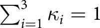 $\sum_{i=1}^{3}\kappa _{i}=1$, and the parameter ρ represents the elasticity of substitution between the energy sources.
Each energy source is produced using sector-specific technologies. Oil reserves, denoted by Rt, are costless to extract.Footnote 1 Oil depletion follows the classic Hotelling (Reference Hotelling1931) rule, under which the net price of oil (price minus extraction cost) rises at the rate of interest. At each point in time, oil extraction satisfies the law of motion:
 \begin{equation}
R_{t+1}=R_{t}-E_{1t},
\end{equation}
where the initial stock R 0 is given.
Coal, although finite, is abundant and does not generate scarcity rents. Both coal and renewable energy are produced using capital and labour according to
 \begin{equation}
E_{it}=f_{it}(A_{it},N_{it},K_{it})\quad \text{for }i=2,3,
\end{equation}
where i = 2 corresponds to coal and i = 3 to renewable energy.
Oil and coal use increase the stock of carbon in the atmosphere, St, while carbon capture reduces it. The economy features two sources of carbon capture: technological carbon capture and natural carbon sinks. The technological carbon capture process removes one unit of carbon using capital and labour, according to the production functionFootnote 2:
 \begin{equation}
f_{it}(A_{it},N_{it},K_{it})\quad \text{for i = 4.}
\end{equation}
Households own the carbon sinks. Individuals derive utility from consumption and experience disutility from labour and from exerting effort, Lt, to preserve carbon sinks. This modelling choice is intended as a simplifying, motivational assumption rather than one with direct policy implications. In fact, at the optimum, it will be true that the marginal cost of capturing carbon from a sink – expressed in terms of foregone utility – must be equal to the shadow value of carbon, just as in the case of technological capture. Both types of carbon removal will share the same social value because they contribute equally to reducing the carbon stock.Footnote 3
Over time, individuals maximise
 \begin{equation}
\sum_{t=0}^{\infty} \beta^{t}[u(C_{t})-v(N_{t})-w(L_{t})]
\end{equation}
where 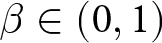 $\beta \in (0,1)$ is the discount factor. Utility functions u, v and w are increasing, concave, twice differentiable, and satisfy Inada conditions. Individuals consume, work, preserve carbon sinks, and invest in capital. Capital depreciates fully within one period and the economy starts with K 0 given.
Oil and coal use increases the stock of carbon in the atmosphere, St, while carbon capture reduces it. Thus, atmospheric carbon evolves following the carbon cycle
 \begin{equation}
S_{t+1}=(1-\gamma )S_{t}+G_{t}-Z_{t},
\end{equation}
where  $Z_{t}=f_{4t}(A_{4t},N_{4t},K_{4t})+L_{t}$ denotes total carbon capture, including both technological and natural sources, and
 $
G_{t}=E_{1t}+\phi E_{2t}$ represents gross emissions. The parameter ϕ captures the relative carbon intensity of coal, with coal typically more polluting than oil. Net emissions are defined as emissions net of carbon capture. The economy begins with an initial carbon stock S 0, and
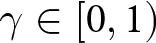 $
\gamma \in \lbrack 0,1)$ denotes the natural rate of carbon absorption.
The stock of carbon in the atmosphere generates a climate externality that takes the form of an output loss. Thus, total output is given by
 \begin{equation}
Y_{t}=F(S_{t},A_{0t},N_{0t},K_{0t},E_{0t})=[1-x(S_{t})]\tilde{F}
(A_{0t},N_{0t},K_{0t},E_{0t}),
\end{equation}
where  $x_{t}(S_{t}$) is a damage function that depends on atmospheric carbon. The function x is increasing, convex and twice differentiable with
 $
\lim_{S\rightarrow \bar{S}}x^{\prime }(S)=0$, where
 $\bar{S}$ is a lower bound on atmospheric CO2 concentration. Also, the sub-index t reflects the possibility that the impact of climate damages may evolve over time. In particular, a given marginal increase in emissions may result in greater damage today than in the future, depending on temporal shifts in vulnerability or the climate system’s responsiveness.
Additionally, total capital and labour used across all sectors must equal the economy’s aggregate capital and labour endowments. Resource feasibility in this economy implies that
 \begin{equation}
C_{t}+K_{t+1}=Y_{t}
\end{equation}
for every period t. Additionally, total capital and labour used across all sectors must equal the economy’s aggregate capital and labour supply:
 \begin{equation}
K_{t}=\sum_{i=0}^{4}K_{it}
\end{equation}
 \begin{equation}
N_{t}=\sum_{i=0}^{4}N_{it},
\end{equation}
for every period t.
Definition 2.1 (Optimal allocation)
The socially optimal allocation is the path of consumption, labour, capital, energy, carbon capture, carbon sinks preservation, and atmospheric carbon,  $
\{C_{t},N_{it},E_{it},K_{it},Z_{t},L_{t},S_{t}\}_{t=0,i=0,1,2,3,4}^{\infty }$, that maximises the welfare function (6) subject to the resource constraints (9)–(11), the carbon cycle (7) and the initial conditions
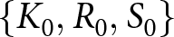 $
\{K_{0},R_{0},S_{0}\}$.
The socially optimal allocation implicitly defines the social cost of carbon, which quantifies the economic cost of the climate externality. Specifically, this cost is derived by forward iteration of the optimality condition for the carbon stock and is given by
 \begin{equation}
\hat{\mu}_{t}\equiv \sum_{h=0}^{\infty }(1-\gamma )^{h}\beta ^{h}\frac{
\lambda _{t+h}}{\lambda _{t}}F_{t,S}^{\prime
}(S_{t+h},A_{0t+h},N_{0t+h},K_{0t+h},E_{0t+h}),
\end{equation}
where λt is the Lagrange multiplier on the feasibility constraint. The social cost of carbon reflects the present value of output losses resulting from one additional unit of atmospheric carbon.
The optimal conditions guarantee production efficiency, including the social cost of carbon. Specifically, production efficiency calls for equalising the marginal productivity of capital and labour – net of the social cost – across productive sectors. In the case of technological carbon capture, the marginal benefit of carbon capture is the avoided climate damages captured in the social cost of carbon, µt, while the marginal cost – the right-hand side of equations (17) and (18) – is the cost of the inputs used in production. Thus, the optimality conditions in the productive sector are:
 \begin{equation}
\lbrack F_{t,E_{2}}^{\prime }-\phi \hat{\mu}_{t}]f_{2t,k}^{\prime
}=F_{t,k}^{\prime }
\end{equation}
 \begin{equation}
\lbrack F_{t,E_{2}}^{\prime }-\phi \hat{\mu}_{t}]f_{2t,n}^{\prime
}=F_{t,n}^{\prime }
\end{equation}
 \begin{equation}
F_{t,E_{3}}^{\prime }f_{3t,k}^{\prime }=F_{t,k}^{\prime }
\end{equation}
 \begin{equation}
F_{t,E_{3}}^{\prime }f_{3t,n}^{\prime }=F_{t,n}^{\prime }
\end{equation}
 \begin{equation}
\hat{\mu}_{t}f_{4_{t,n}}^{\prime }=F_{t,n}^{\prime }
\end{equation}
 \begin{equation}
\hat{\mu}_{t}f_{4t,k}^{\prime }=F_{t,k}^{\prime }.
\end{equation}
For ease of notation, the arguments of the production functions are omitted. All expressions and conditions are evaluated at time t. The first subscript denotes the time-dependence of the function, while the second subscript indicates the variable with respect to which the function is being differentiated. For example,  $F_{t,E_{2}}^{\prime }$ denotes the derivative of the final goods production function with respect to coal input, E 2, evaluated at time t. The same notation is followed throughout the paper. Moreover, we denote
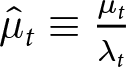 $\hat{\mu}_{t}\equiv \frac{\mu _{t}}{\lambda _{t}}$.
Since oil is an exhaustible resource, its efficient use is governed by the classic Hotelling rule (Hotelling, Reference Hotelling1931), which balances the intertemporal value of oil extraction. In this case, the marginal benefit from extracting an additional unit of oil today must equal the discounted marginal benefit of extraction tomorrow:
 \begin{equation}
\beta u^{\prime }(C_{t+1})[F_{t+1,E_{1}}-\hat{\mu}_{t+1}]=u^{\prime
}(C_{t})[F_{t,E_{1}}-\hat{\mu}_{t}],
\end{equation}
where  $F_{t,E_{1}}$ denotes the marginal product of oil net of the associated climate damages, µt.
In addition, an arbitrage condition equates the returns on oil and productive capital since both serve as saving assets in this economy. This condition ensures that both capital and oil reserves yield the same return:
 \begin{equation}
\frac{F_{t+1,E_{1}}-\hat{\mu}_{t+1}}{F_{t,E_{1}}-\hat{\mu}_{t}}=F_{t+1,k},
\end{equation}
where  $F_{t+1,k}$ is the marginal product of capital evaluated at t + 1.
On the intratemporal margin, the model features a standard trade-off between labour and consumption. Specifically, the marginal rate of substitution between leisure and consumption equals the marginal rate of transformation:
 \begin{equation}
\frac{v^{\prime }(N_{t})}{u^{\prime }(C_{t})}=F_{t,n}^{\prime },
\end{equation}
where  $v(N_{t})$ is the disutility of labour and
 $F_{t,n}^{\prime }$ is the marginal product of labour evaluated at t.
Finally, the optimal allocation internalises the benefits of preserving carbon sinks. Efforts to preserve or expand carbon sinks divert resources away from productive activities. At the margin, the effort allocated to maintaining or expanding carbon sinks must equal their social value, which is the avoided climate damages captured by the social cost of carbon:
 \begin{equation}
\frac{\omega ^{\prime }(L_{t})}{u^{\prime }(C_{t})}=\hat{\mu}_{t},
\end{equation}
where  $\omega (L_{t})$ denotes the cost function associated with carbon sink preservation.
The socially optimal allocation satisfies equations (13)–(22) together with resource feasibility (9)–(11) and the transversality conditions for capital and oil reserves.
3. Optimal carbon markets
Consider a market equilibrium with carbon taxes and a market for carbon credits. Carbon taxes include a tax on emissions, τt, and subsidies for carbon capture,  $\tau_t^z$, carbon sink preservation,
 $
\tau_t^\ell$, and renewable energy,
 $\tau_t^r$. In the carbon credit market, households and firms trade credits. The seller of a carbon credit commits to capture one unit of atmospheric carbon, either through natural resources or technologically.
In the energy sector, oil and coal firms may purchase carbon credits to offset their emissions. The oil firm (i = 1) chooses an extraction path to maximise discounted profits:
 \begin{equation}
\Pi _{1}=\sum_{t=0}^{\infty }q_{t}^{0}[p_{1t}E_{1t}-\tau
_{t}(E_{1t}-z_{1t})-p_{t}^{z}z_{1t}],
\end{equation}
subject to the depletion equation (3) and initial oil reserves R 0, where  $p_{1t}$ is the price of oil in consumption units and
 $z_{1t}$ are carbon credits purchased by the oil firm.
The coal firm (i = 2) operates technology (4) and pays a carbon tax τt on coal-related emissions. It chooses inputs  $
\{N_{2t},K_{2t}\}_{t=0}^{\infty }$ to maximise
 \begin{equation}
\Pi _{2}=\sum_{t=0}^{\infty }q_{t}^{0}[p_{2t}E_{2t}-\tau _{t}(\phi
E_{2t}-z_{2t})-w_{t}N_{2t}-r_{t}K_{2t}-p_{t}^{z}z_{2t}],
\end{equation}
where  $p_{2t}$ is the coal price in consumption units and
 $z_{2t}$ are carbon credits purchased by the coal firm.
The renewable energy firm (i = 3) operates technology (4) and receives a subsidy  $\tau _{t}^{r}$ per unit of output. It maximises
 \begin{equation}
\Pi _{3}=\sum_{t=0}^{\infty }q_{t}^{0}[(p_{3t}+\tau
_{t}^{r})E_{3t}-w_{t}N_{3t}-r_{t}K_{3t}].
\end{equation}
The final goods producer hires labour at wage wt, rents capital at rate rt, and purchases energy from the energy firms at prices pit. It chooses  $\{K_{0t},N_{0t},E_{1t},E_{2t},E_{3t}\}_{t=0}^{\infty }$ to maximise
 \begin{equation}
\Pi _{0}=\sum_{t=0}^{\infty
}q_{t}^{0}[F(A_{0t},S_{t},N_{0t},K_{0t},E_{0t})-r_{t}K_{0t}-w_{t}N_{0t}-
\sum_{i=1}^{3}p_{it}E_{it}],
\end{equation}
where  $q_{t}^{0}$ is the Arrow-Debreu price of consumption in period t relative to period 0.
Carbon capture firms operate technology (5) and receive a subsidy  $
\tau _{t}^{z}$ per unit captured. They hire labour and rent capital to maximise
 \begin{equation}
\Pi _{4}=\sum_{t=0}^{\infty }q_{t}^{0}[(p_{t}^{z}+\tau
_{t}^{z})f_{4}(A_{4t},N_{4t},K_{4t})-w_{t}N_{4t}-r_{t}K_{4t}],
\end{equation}
where  $p_{t}^{z}$ is the price of carbon capture in consumption units.
The representative household owns firms and carbon sinks, supplies labour, consumes, preserves carbon sinks, and saves. The household faces the present value budget constraint,
 \begin{equation}
\sum_{t=0}^{\infty }q_{t}^{0}[C_{t}+K_{t+1}]\leq \sum_{t=0}^{\infty
}q_{t}^{0}[r_{t}K_{t}+w_{t}N_{t}+(p_{t}^{z}+\tau _{t}^{\ell
})L_{t}+T_{t}]+\Pi ,
\end{equation}
where 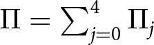 $\Pi =\sum_{j=0}^{4}\Pi _{j}$ are firm dividends,
 $\tau _{t}^{\ell }$ is the subsidy for carbon sinks preservation, Tt is a lump-sum tax/rebate, and K 0 is the initial capital stock. Households choose
 $
\{C_{t},N_{t},L_{t},K_{t}\}_{t=0}^{\infty }$ to maximise (6) subject to (28), taking prices and taxes as given.
The government collects taxes and rebates any surplus lump sum to households. Its budget constraint is
 \begin{equation}
\sum_{t=0}^{\infty }q_{t}^{0}[\tau _{t}(E_{1t}+\phi
E_{2t})]=\sum_{t=0}^{\infty }q_{t}^{0}[\tau
_{t}^{z}f_{4t}(A_{4t},N_{4t},K_{4t})+\tau _{t}^{\ell }L_{t}+\tau
_{t}^{r}E_{3t}+T_{t}].
\end{equation}
Market clearing requires (9)–(11) to hold together with the following condition for carbon capture markets:
 \begin{equation}
\sum_{i=1}^{2}z_{it}=Z_{t}
\end{equation}
for all t, where  $Z_{t}=f_{4t}(A_{4t},N_{4t},K_{4t})+L_{t}$ denotes total carbon capture, including both technological and natural sources.
Definition 3.1 (Competitive equilibrium)
A competitive equilibrium given fiscal policy  $\left\{\tau_{t},
\tau_{t}^{z},\tau_{t}^{\ell},\tau_{t}^{r},T_{t}\right\} _{t=0}^{\infty }$ is an allocation
 $\left\{C_{t},N_{it},E_{it},K_{it},Z_{t},L_{t},S_{t}\right
\} _{t=0,i=0,...,4}^{\infty }$ and a sequence of prices
 $\left
\{q_{t}^{0},p_{it},p_{t}^{z},r_{t},w_{t}\right\} _{t=0,i=1,...,4}^{\infty }$ such that:
 $\left( i\right) $ given the fiscal policy and prices, the allocation solves the consumer’s problem, maximising (6) subject to (28), and the firms’ problems, maximising
 $
\Pi_{i}$ for i={0,...,4};
 $\left( ii\right) $ the government budget constraint
 $\left(29\right) $ is satisfied;
 $\left( iii\right) $ the carbon stock follows the carbon cycle (7); and
 $\left(
iv\right) $ prices clear markets.
At an interior solution, profit maximisation by the final goods producer implies that factor prices equal marginal products:
 \begin{equation}
F^{\prime}_{t,n}=w_{t}, \quad F^{\prime}_{t,k}=r_{t}, \quad
F^{\prime}_{t,E_{j}}=p_{jt}, \quad j=1,2,3.
\end{equation}
Likewise, production efficiency requires that factor prices equal marginal products in the coal and renewable energy sectors:
 \begin{align}
(p_{2t}-\phi \tau _{t})f_{2t,k}^{\prime }& =r_{t},\quad (p_{2t}-\phi \tau
_{t})f_{2t,n}^{\prime }=w_{t},
\end{align}
 \begin{align}
(p_{3t}+\tau _{t}^{r})f_{3t,k}^{\prime }& =r_{t},\quad (p_{3t}+\tau
_{t}^{r})f_{3t,n}^{\prime }=w_{t},
\end{align}
and in the carbon capture sector:
 \begin{equation}
(p_{t}^{z}+\tau _{t}^{z})f_{4t,n}^{\prime }=w_{t},\quad (p_{t}^{z}+\tau
_{t}^{z})f_{4t,k}^{\prime }=r_{t}.
\end{equation}
Profit maximisation in the oil and coal industries implies the following condition on carbon credit prices:
 \begin{equation}
p_{t}^{z}=\tau _{t}.
\end{equation}
For oil firms, the Hotelling rule ensures that the return on oil extraction is equalised over time:
 \begin{equation}
q_{t+1}^{0}(p_{1t+1}-\tau _{t+1})=q_{t}^{0}(p_{1t}-\tau _{t}),
\end{equation}
where Arrow-Debreu prices satisfy:
 \begin{equation}
q_{t}^{0}=\beta ^{t}\frac{u^{\prime }(C_{t})}{u^{\prime }(C_{0})},\quad
q_{0}^{0}=1.
\end{equation}
Substituting (37) and 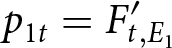 $p_{1t}=F_{t,E_{1}}^{\prime }$ yields
 \begin{equation}
\beta u^{\prime }(C_{t+1})(F_{t+1,E_{1}}^{\prime }-\tau _{t+1})=u^{\prime
}(C_{t})(F_{t,E_{1}}^{\prime }-\tau _{t}).
\end{equation}
This condition shows that the oil return equals its marginal productivity net of taxes.
On the household side, the Euler equation characterises optimal saving:
 \begin{equation}
\beta u^{\prime}(C_{t+1}) r_{t+1} = u^{\prime}(C_{t}).
\end{equation}
Combining (38) and (39) implies a no-arbitrage condition equating returns on capital and oil:
 \begin{equation}
F^{\prime}_{t+1,k} = \frac{F^{\prime}_{t+1,E_{1}} - \tau_{t+1}}{
F^{\prime}_{t,E_{1}} - \tau_{t}}.
\end{equation}
The household’s intratemporal conditions equate marginal rates of substitution to relative prices:
 \begin{equation}
\frac{v^{\prime }(N_{t})}{u^{\prime }(C_{t})}=w_{t},\quad \frac{\omega
^{\prime }(L_{t})}{u^{\prime }(C_{t})}=p_{t}^{z}+\tau _{t}^{\ell }.
\end{equation}
In sum, the competitive equilibrium is characterised by the intertemporal conditions (38), (39), the intratemporal conditions (32)–(33), (34), (41) together with prices that satisfy (31), (37), (35), market clearing (9)–(11), and the transversality conditions on capital and oil stocks.
3.1. Business-as-usual carbon capture
Condition (35) implies that a market for carbon capture operates only when carbon taxes are in place. In a business-as-usual economy without such taxes, the price of carbon capture credits falls to zero, and no carbon capture firms are active. Likewise, there is no trading of credits from natural carbon sinks. The household optimality condition (41) further indicates that, absent tax incentives, no effort is exerted to preserve natural carbon sinks. Nonetheless, carbon emissions from natural sinks may still occur passively.
Indeed, natural carbon sinks continue to absorb carbon as part of the natural cycle, as described by equation (7), even in the absence of explicit market mechanisms. However, without preservation efforts, the stock of these sinks will generally fall short of the socially optimal level. In contrast to technological carbon capture, which requires explicit policy incentives, natural carbon sinks provide climate benefits – lower atmospheric carbon concentrations and avoided damage – at no direct cost to the market. These unpriced benefits exist independently of formal carbon markets. Whether or not natural sinks should be credited only for efforts beyond their baseline capacity is key in determining whether additionality constraints should be imposed in a carbon market.
3.2. Optimal carbon prices
The following proposition presents the main result of the paper, highlighting the core mechanism behind carbon pricing. It shows that a carbon tax effectively implements a carbon market. In this market, every activity that emits or removes carbon from the atmosphere carries a price. The proposition demonstrates that the carbon tax alone helps internalise both the social cost of emissions and the social value of carbon capture. As a result, subsidies aimed at preserving carbon sinks or supporting carbon capture technologies are redundant. In equilibrium, the price of carbon capture equals the carbon tax. The proof is included in the appendix.
Proposition 3.2 (Optimal carbon prices)
Let  $\{C_{t},N_{it},E_{it},Z_{t},L_{t},K_{it},S_{t}
\}_{t=0,i=0,...,4}^{\infty }$ be the socially optimal allocation. Then, there exists a sequence of prices such that this allocation is a competitive equilibrium with taxes given by
 \begin{equation}
\tau {_{t}}=\hat{\mu}_{t}
\end{equation}
and
 \begin{equation}
\tau _{t}^{z}=\tau _{t}^{r}=\tau _{t}^{\ell }=0
\end{equation}
for every period t. Any fiscal surplus is rebated as a lump sum through Tt.
In the carbon market equilibrium, carbon capture is priced at its social value. Carbon capture has value because it reduces atmospheric carbon, avoiding future climate damages inasmuch as reducing carbon emissions does. Importantly, the optimal policy framework does not require the concept of ‘additionality’ as a condition for pricing. On the contrary, the analysis shows that every unit of carbon captured – regardless of whether it exceeds a baseline or not – should receive a uniform price equal to the social cost of carbon, 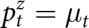 $p_{t}^{z}=\mu
_{t}$.
This result directly challenges the design of current voluntary carbon markets, where credits are often awarded only for activities deemed additional – i.e., beyond what would have occurred under business-as-usual. Such a requirement implies that some beneficial carbon capture must be provided ‘for free’, while all carbon emissions are subject to a price. This asymmetry lacks an economic justification and likely leads to under-provision of equilibrium carbon capture. The following corollary formalises this insight.
Corollary 3.3 (No additionality requirement)
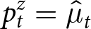 $p_{t}^{z}=\hat{\mu}_{t}$ for all
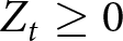 $Z_{t}\geq 0$.
Corollary 3.3 states that the price of carbon capture is equal to the social cost of carbon for all levels and types of capture. This applies equally to natural carbon sinks (e.g., forests, wetlands, soils) and to technological carbon removal (e.g., direct air capture or CCS). For this mechanism to function properly, measurement and monitoring of carbon capture sources and clear property rights over carbon sinks must be established. In the model, households own the sinks; in practice, sinks are often managed by governments, which can license or regulate access to the carbon removal services they provide.
3.3. Carbon capture capacity constraints: an extension
Implementing carbon capture faces several practical challenges. Technological solutions are often hindered by high upfront costs and uncertain returns. Nature-based solutions require accurate measurement and verification of sequestered carbon, which in turn depend on robust monitoring, reporting, and verification (MRV) systems that are still underdeveloped. A further concern is permanence – ensuring that captured carbon is not subsequently released through leakage or land-use change.
To incorporate these constraints, an extension of the model introduces a carbon capture storage variable,  $\hat{W}_{t}$. At each point in time, captured carbon is added to this stock,
 \begin{equation}
\hat{W}_{t+1}=\hat{W}_{t}+Z_{t},
\end{equation}
subject to an upper bound on storage capacity:
 \begin{equation}
\hat{W}_{t+1}\leq \bar{W}.
\end{equation}
Let  $\beta ^{t}\delta _{t}$ and
 $\beta ^{t}\kappa _{t}$ denote the Lagrange multiplier associated with constraints (44) and (45), respectively. For clarity, assume that all carbon capture is from natural sinks, Lt. The first-order condition becomes
 \begin{equation*}
(L_{t}):-\beta ^{t}\omega ^{\prime }(L_{t})-\beta ^{t}\mu _{t}-\beta
^{t}\delta _{t}=0
\end{equation*}
together with
 \begin{equation*}
(W_{t+1}):\beta ^{t}\delta _{t}-\beta ^{t+1}\delta _{t+1}-\beta ^{t}\kappa
_{t}=0,
\end{equation*}
which yields the modified optimality condition
 \begin{equation}
\frac{\omega (L_{t})}{u(C_{t})}=\hat{\mu}_{t}+\sum_{h=0}^{\infty }\frac{
\beta ^{h}\kappa _{t+h}}{\lambda _{t}}.
\end{equation}
The right-hand side of (46) now includes two terms. The first,  $
\hat{\mu}_t$, represents the marginal climate damages avoided through carbon removal (as in equation (12)). The second captures the Hotelling-type scarcity value of carbon storage capacity. This term is zero if constraint (45) never binds; otherwise, it adds a dynamic scarcity rent that grows at the rate of interest, akin to the classic Hotelling rule for exhaustible resources.
In addition to physical storage constraints, further extensions could incorporate the non-permanence of carbon capture, as well as monitoring costs. A recent paper by Kalkuhl et al. (Reference Kalkuhl, Franks, Gruner, Lessmann and Edenhofer2022) analyses a related framework in which carbon capture is non-permanent and serves as a transitional solution towards permanent removal. In their model, carbon captured today is released back into the atmosphere at some point in the future. The paper shows that the price of carbon capture is modified to incorporate two components: the marginal damage resulting from releasing emissions from storage back into the atmosphere, and the marginal cost of controlling the timing of carbon re-release from temporary storage.
Even when the perfect implementation of carbon pricing is not feasible, the main result of the paper remains: subsidies for carbon capture, payments for sink preservation, and ‘additionality’ criteria are second-best instruments. They become relevant only in the absence of a comprehensive, global carbon price.
3.4. Discussion and policy implications
Pricing carbon capture and incorporating it into a comprehensive carbon pricing system has been difficult due to challenges in measurement and a lack of consistent standards. For example, forest preservation is often seen as a public good that countries must provide. Projects aimed at conserving forests, which absorb CO2 and store it in soil, must show that the land would not have been preserved under business-as-usual conditions.
Developing countries hold a significant share of the world’s nature-based carbon capture resources, including the Amazon rainforest, peatlands, soils and freshwater reservoirs. Their ability to count the carbon sequestered within their territories towards their nationally determined contributions (NDCs), or to sell credits in international carbon markets, is central to determining whether they can contribute fairly and effectively to the global transition towards a low-carbon economy.
This issue connects to broader debates on climate justice (Shue, Reference Shue2014; McKinnon, Reference McKinnon2015; Skeie et al., Reference Skeie, Fuglestvedt, Berntsen, Peters, Andrew, Allen and Kallbekken2017), which emphasise the tension between historical responsibility, persistent global inequalities and the urgency of climate action. High-income countries have historically relied on fossil fuels to drive economic growth and account for the bulk of cumulative emissions, while many low-income countries are still pursuing development. Addressing fairness and equity in climate policy requires innovative mechanisms that balance environmental effectiveness with developmental needs. Carbon capture can serve this dual purpose: it allows high-income countries to offset past emissions, while also giving low-income countries more time to grow – and new economic opportunities through participation in carbon markets and sequestration initiatives.
In related work, Belfiori and Macera (Reference Belfiori and Macera2024) contribute to this discussion by analysing optimal emissions and carbon capture targets in a world with heterogeneous regions. They show that achieving global net-zero emissions efficiently requires high-income countries to pursue net-negative emissions – through both technological and natural carbon capture – while low-income countries continue to emit on net for a longer period. This result highlights the role of carbon capture not only as a mitigation tool, but also as a redistributive mechanism within a global carbon pricing system.
Recognising these asymmetries is essential for designing climate policies that balance efficiency and equity. Yet in all scenarios, a necessary first step is to establish a clear and credible market price for carbon capture. Such a price is critical for creating the right incentives to invest in both technological removal and the conservation of natural carbon sinks.
Voluntary carbon markets have responded to these challenges by relying on the ‘additionality’ criterion, which only rewards carbon removal activities that exceed a baseline scenario. Yet, as shown by Proposition 3.2 and its corollary, this approach creates a fundamental asymmetry: emissions are taxed unconditionally, while carbon removal is credited only when it is deemed ‘additional’. This raises an important question: why should a country pay for every ton of emissions it releases but receive credits only for carbon captured beyond a certain threshold?
This is where the concept of ‘additionality’ becomes problematic. It assumes that a portion of nature-based carbon capture, which occurs naturally, must be provided at no cost, without generating carbon credits. This assumption weakens efforts to safeguard global public goods and limits the ability of developing countries to fully participate in climate policy.
Proposition 3.2 shows that, within an optimal carbon market, every ton of carbon removed – regardless of whether it exceeds a baseline – has the same social value and should receive the same price. Eliminating the additionality requirement and pricing all non-negative carbon removal equally aligns incentives, removes distortions, and allows developing countries to participate more fully and fairly in global climate policy. Many of these countries possess vast natural sinks, and the ability to receive a fair price for the global public goods they provide is crucial for achieving a level playing field in mitigation efforts across countries and technologies.
Despite the challenges and caveats, establishing a carbon price for carbon capture is essential. It provides the foundation for aligning incentives with climate goals, strengthening measurement and monitoring systems, encouraging innovation, and ultimately enabling compliance with the climate targets set by the Paris Agreement – which by now will unequivocally require the deployment of carbon removal at scale.
4. Conclusions
Setting a price for carbon capture is crucial for developing countries, as it ensures they can participate meaningfully in global climate mitigation efforts. A price for carbon capture is necessary.Footnote 4
This paper develops a global economic model with carbon markets that incorporate carbon-intensive energy sources, renewable energy, natural carbon sinks, and carbon capture technologies. The main result shows that a carbon tax alone can generate an efficient carbon market in which emissions, carbon sink preservation, and all forms of carbon capture are priced equally.
Using this model, we argue that ‘additionality’ is not a necessary condition for optimal carbon pricing. On the contrary, all non-negative carbon removal efforts should be priced uniformly at the social cost of carbon – the present value of the climate damages avoided by removing one unit of atmospheric carbon.
The analysis implies that additionality requirements, subsidies for carbon capture, payments for sink preservation, and even some conservation laws, are all second-best instruments. These measures become relevant only when a comprehensive global carbon price is absent. Relying on such a second-best policies carry the risk of implementing measures that create the appearance of progress but fall short of reaching the necessary climate goals. Accurately pricing both positive and negative emissions is fundamental to achieving efficient and equitable climate mitigation.
Acknowledgements
The author thanks Yanel Llohis for outstanding research assistance.
Competing interests
The author declares none.
Appendix A. Characterisation of the optimal allocation
In this section, we provide the complete solution to the problem solved to find the optimal allocation defined in definition 1. The Lagrangian associated with the problem of maximising the welfare function (6) subject to the resource constraints (9)–(11), the carbon cycle (7) and the initial conditions 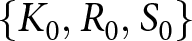 $\{K_{0},R_{0},S_{0}\}$ is the following:
 \begin{align*}
& \mathcal{L}:\sum_{t=0}^{\infty }\beta
^{t}[u(C_{t})-v(N_{t})-w(L_{t})]-\beta ^{t}\lambda _{t}\left[
C_{t}+K_{t+1}-F_{t}(S_{t},A_{0t},N_{0t},K_{0t},E_{0t})\right] \\
& \quad -\beta ^{t}\mu _{t}\left[ (1-\gamma )S_{t}+(R_{t}-R_{t+1})+\phi
f_{2t}(A_{2,t},N_{2,t},K_{2,t)}-f_{4t}(A_{4t},N_{4t},K_{4t})+L_{t}-S_{t+1}
\right] .
\end{align*}
And the first-order conditions are:
 \begin{equation}
\!\!\!\!\!\!\!\!\!\!\!\!\!\!\!\!\!\!\!\!\!\!\!\!\!\!\!\!\!\!\!\!\!\!\!\!\!\!\!\!\!\!\!\!\!\!\!\!\!\!\!\!\!\!\!\!\!\!\!\!\!\!\!\!\!\!\!\!\!\!\!\!\!\!\!\!\!\!\!\!\!\!\!\!\!\!\!\!\!\!\!\!\!\!\!\!\! (C_{t}):\beta ^{t}u^{\prime }(C_{t})-\beta ^{t}\lambda _{t}=0
\end{equation}
 \begin{equation}
\!\!\!\!\!\!\!\!\!\!\!\!\!\!\!\!\!\!\!\!\!\!\!\!\!\!\!\!\!\!\!\!\!\!\!\!\!\!\!\!\!\!\!\!\!\!\!\!\!\!\!\!\!\!\!\!\!\!\!\!\!\!\!\!\!\!(K_{0,t+1}):-\beta ^{t}\lambda _{t}+\beta ^{t+1}\lambda
_{t+1}F_{t+1,k}^{\prime }=0
\end{equation}
 \begin{equation}
(K_{2,t+1}):-\beta ^{t}\lambda _{t}+\beta ^{t+1}\lambda
_{t+1}F_{t+1,E_{2}}^{\prime }{f_{2t+1,k}^{\prime }}-\beta ^{t+1}\mu
_{t+1}\phi {f_{2t+1,k}^{\prime }}=0
\end{equation}
 \begin{equation}
\!\!\!\!\!\!\!\!\!\!\!\!\!\!\!\!\!\!\!\!\!\!\!\!\!\!\!\!\!\!\!\!\!\!\!\!\!\!\!\!\!\!\!\!\!\!\!\!\!(K_{3,t+1}):-\beta ^{t}\lambda _{t}+\beta ^{t+1}\lambda
_{t+1}F_{t+1,E_{3}}^{\prime }{f_{3t+1,k}^{\prime }}=0
\end{equation}
 \begin{equation}
\!\!\!\!\!\!\!\!\!\!\!\!\!\!\!\!\!\!\!\!\!\!\!\!\!\!\!\!\!\!\!\!\!\!\!\!\!\!\!\!\!\!\!\!\!\!\!\!\!\!\!\!\!\!\!\!\!\!\!\!\!\!\!\!\!\!(K_{4,t+1}):-\beta ^{t}\lambda _{t}+\beta ^{t+1}\mu
_{t+1}f_{4t+1,k}^{\prime }=0
\end{equation}
 \begin{equation}
\!\!\!\!\!\!\!\!\!\!\!\!\!\!\!\!\!\!\!\!\!\!\!\!\!\!\!\!\!\!\!\!\!\!\!\!\!\!\!\!\!\!\!\!\!\!\!\!\!\!\!\!\!\!\!\!\!\!\!\!\!\!\!\!\!\!\!\!\!\!\!\!\!\!\!\!\!\!(N_{0,t}):-\beta ^{t}\nu ^{\prime }(N_{t})+\beta ^{t}\lambda
_{t}F_{t,n}^{\prime }=0
\end{equation}
 \begin{equation}
\!\!\!\!\!\!\!\!\!\!\!\!\!\!\!\!\!\!\!\!\!\!\!\!\!\!\!\!\!\!\!\!\!(N_{2,t}):-\beta _{t}\nu ^{\prime }(N_{t})+\beta ^{t}\lambda
_{t}F_{t,E_{2}}^{\prime }f_{2t,n}^{\prime }-\beta ^{t}\mu _{t}\phi
f_{2t,n}^{\prime }=0
\end{equation}
 \begin{equation}
\!\!\!\!\!\!\!\!\!\!\!\!\!\!\!\!\!\!\!\!\!\!\!\!\!\!\!\!\!\!\!\!\!\!\!\!\!\!\!\!\!\!\!\!\!\!\!\!\!\!\!\!\!\!\!\!\!\!\!\!\!\!\!\!\!(N_{3,t}):-\beta ^{t}\nu ^{\prime }(N_{t})+\beta ^{t}\lambda
_{t}F_{t,E_{3}}^{\prime }f_{3t,n}^{\prime }=0
\end{equation}
 \begin{equation}
\!\!\!\!\!\!\!\!\!\!\!\!\!\!\!\!\!\!\!\!\!\!\!\!\!\!\!\!\!\!\!\!\!\!\!\!\!\!\!\!\!\!\!\!\!\!\!\!\!\!\!\!\!\!\!\!\!\!\!\!\!\!\!\!\!\!\!\!\!\!\!\!\!\!\!\!(N_{4,t}):-\beta ^{t}\nu ^{\prime }(N_{t})+\beta ^{t}\mu
_{t}f_{4t,n}^{\prime }=0
\end{equation}
 \begin{equation}
\!\!\!\!\!\!\!\!\!\!\!\!\!\!\!\!\!\!\!\!\!\!\!\!\!\!(S_{t+1}):\beta ^{t}\mu _{t}-\beta ^{t+1}\mu _{t+1}(1-\gamma )+\beta
^{t+1}\lambda _{t+1}F_{t+1,S}^{\prime }=0
\end{equation}
 \begin{equation}
\!\!\!\!\!\!\!\!\!\!\!\!\!\!\!\!\!\!\!\!\!\!\!\!\!\!\!\!\!\!\!\!\!\!\!\!\!\!\!\!\!\!\!\!\!\!\!\!\!\!\!\!\!\!\!\!\!\!\!\!\!\!\!\!\!\!\!\!\!\!\!\!\!\!\!\!\!\!\!\!\!\!\!\!\!\!\!\!\!\!\!\!(L_{t}):-\beta ^{t}\omega ^{\prime }(L_{t})-\beta ^{t}\mu _{t}=0
\end{equation}
 \begin{equation}
\!\!\!\!\!\!(R_{t+1}):-\beta ^{t}\lambda _{t}F_{t,E_{1}}^{\prime }+\beta ^{t}\mu
_{t}+\beta ^{t+1}\lambda _{t+1}F_{t+1,E_{1}}^{\prime }-\beta ^{t+1}\mu
_{t+1}=0.
\end{equation}
For ease of notation, the arguments of the production functions are omitted. All expressions and conditions are evaluated at time t. The first subscript denotes the time-dependence of the function, while the second subscript indicates the variable with respect to which the function is being differentiated. For example,  $F_{t,E_{2}}^{\prime }$ denotes the derivative of the final goods production function with respect to coal input, E 2, evaluated at time t.
We will show that the first-order conditions (A.1)–(A.12) combined yield the optimality conditions (13)–(22) that characterise the socially optimal allocation together with the transversality conditions for capital and oil reserves.
Let us denote 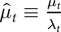 $\hat{\mu}_{t}\equiv \frac{\mu _{t}}{\lambda _{t}}$. Combining equations (A.2) and (A.3) yields equation (13)
 \begin{equation*}
{f_{2}^{\prime }}_{K_{2,t}}(F_{E_{2,t}}^{\prime }-\phi \hat{\mu}
_{t})=F_{K_{t}}^{\prime },
\end{equation*}
and similarly, equation (14) can be obtained combining (A.6) and (A.7),
 \begin{equation*}
f_{2t,n}^{\prime }(F_{t,E_{2}}^{\prime }-\phi \hat{\mu}_{t})=F_{t,n}^{\prime
}.
\end{equation*}
Combining equations (A.2) and (A.4) yields equation (15),
 \begin{equation*}
F_{t,E_{3}}^{\prime }f_{3t,k}^{\prime }=F_{t,k}^{\prime },
\end{equation*}
and combining (A.6) and (A.8) yields equation (16),
 \begin{equation*}
F_{t,E_{3}}^{\prime }f_{3t,n}^{\prime }=F_{t,n}^{\prime }.
\end{equation*}
Equation (17) can be derived by combining equations (A.6) and (A.9):
 \begin{equation}
\hat{\mu}_{t}f_{4t,n}^{\prime }=F_{t,n}^{\prime },
\end{equation}
and (A.2) and (A.5) combined yield equation (18) ,
 \begin{equation}
\hat{\mu}_{t}f_{4t,k}^{\prime }=F_{t,k}^{\prime }.
\end{equation}
Equation (19) can be derived from the combining of (A.12) and (A.1):
 \begin{equation*}
\beta u^{\prime }(C_{t+1})(F_{t+1,E_{1}}^{\prime }-\hat{\mu}
_{t+1})=u^{\prime }(C_{t})(F_{t,E_{1}}^{\prime }-\hat{\mu}_{t}),
\end{equation*}
and combining this with (A.2) yields equation (20):
 \begin{equation*}
\frac{F_{t+1,E_{1}}-\hat{\mu}_{t+1}}{F_{t,E_{1}}-\hat{\mu}_{t}}=F_{t+1,k}.
\end{equation*}
Finally, dividing (A.6) by (A.1) yields (21):
 \begin{equation}
\frac{\nu ^{\prime }(N_{t})}{u^{\prime }(C_{t})}=F_{t,n}^{\prime },
\end{equation}
and dividing (A.11) by(A.1) gives (22):
 \begin{equation*}
\frac{\omega ^{\prime }(L_{t})}{u^{\prime }(C_{t})}=\hat{\mu}_{t}.
\end{equation*}
B. Characterisation of the market equilibrium
We show that the competitive equilibrium is characterised by two intertemporal conditions (38), (39), the production optimality conditions (32)–(33) and (34), the intratemporal condition (41) together with prices that satisfy ( 31), (37), (35), market clearing (9)–(11), and the transversality conditions on capital and oil stocks.
Oil sector: The representative firm in the oil sector (i = 1) solves
 \begin{equation*}
\max_{R_{t+1},z_{t}}\sum_{t=0}^{\infty }q_{t}^{0}\left[
p_{1,t}(R_{t}-R_{t+1})-\tau _{t}(R_{t}-R_{t+1}-z_{1,t})-p_{t}^{z}z_{1,t}
\right] .
\end{equation*}
And the first-order conditions with respect to  $R_{t+1}$ and zt yield equations (35) and (36) respectively,
 \begin{align}
\quad(R_{t+1}):q_{t}^{0}(p_{1,t}-\tau _{t})=q_{t+1}^{0}(p_{1,t+1}-\tau _{t+1}),
\end{align}
 \begin{equation}
\!\!\!\!\!\!\!\!\!\!\!\!\!\!\!\!\!\!\!\!\!\!\!\!\!\!\!\!\!\!\!\!\!\!\!\!\!\!\!\!\!\!\!\!\!\!\!\!\!\!\!\!\!\!\!\!\!\!\!\!\!\!\!\!\!\!\!\!\!(z_{t}):\tau _{t}=p_{t}^{z}.
\end{equation}
Coal sector: The representative firm in the coal sector solves
 \begin{equation}
\max_{N_{2,t},K_{2,t},z_{t}}\sum_{t=0}^{\infty }q_{t}^{0}[p_{2t}E_{2t}-\tau
_{t}(\phi E_{2t}-z_{2t})-w_{t}N_{2t}-r_{t}K_{2t}-p_{t}^{z}z_{2t}],
\end{equation}
and the first-order conditions yield equations (32) and (35):
 \begin{align*}
& (K_{2,t}):(p_{2t}-\phi \tau _{t})F_{2t,k}^{\prime }=r_{t} \\
& (N_{2,t}):(p_{2t}-\phi \tau _{t})F_{2t,n}^{\prime }=w_{t} \\
& (z_{t}):\tau _{t}=p_{t}^{z}.
\end{align*}
Renewable energy sector: The representative firm in the renewable energy sector solves
 \begin{equation}
\max_{N_{3,t},K_{3,t}}\sum_{t=0}^{\infty }q_{t}^{0}[(p_{3t}+\tau
_{t}^{r})f_{3t}(A_{3t},N_{3t},K_{3t})-w_{t}N_{3t}-r_{t}K_{3t}],
\end{equation}
and the first-order conditions yield equations (33),
 \begin{align*}
& (K_{3,t}):(p_{3t}+\tau _{t}^{r})F_{3t,k}^{\prime }=r_{t} \\
& (N_{3,t}):(p_{3t}+\tau _{t}^{r})F_{3t,n}^{\prime }=w_{t}.
\end{align*}
Final good sector: The firm producing the final good solves
 \begin{equation}
\max_{N_{0,t},K_{0,t},E_{1,t},E_{2,t},E_{3,t}}\sum_{t=0}^{\infty
}q_{t}^{0}[F_{t}(A_{0t},S_{t},N_{0t},K_{0t},E_{0t})-r_{t}K_{0t}-w_{t}N_{0t}-
\sum_{i=1}^{3}p_{it}E_{it}],
\end{equation}
and the first-order conditions yield equations (31),
 \begin{align*}
& (N_{0,t}):F_{t,n}^{\prime }=w_{t} \\
& (K_{0,t}):F_{t,k}^{\prime }=r_{t} \\
& (E_{j,t}):F_{t,E_{j}}^{\prime }=p_{jt}\,\,\text{for }j=1,2,3.
\end{align*}
Carbon capture sector: The firm that captures carbon solves
 \begin{equation*}
\max_{N_{4,t},K_{4,t}}\sum_{t=0}^{\infty }q_{t}^{0}[(p_{t}^{z}+\tau
_{t}^{z})f_{4t}(A_{4t},N_{4t},K_{4t})-w_{t}N_{4t}-r_{t}K_{4t}]
\end{equation*}
and first-order conditions give equations (34),
 \begin{align*}
& (N_{4,t}):(p_{t}^{z}+\tau _{t}^{z})\,\,f_{4t,n}^{\prime }(t)=w_{t} \\
& (K_{4,t}):(p_{t}^{z}+\tau _{t}^{z})\,\,f_{4t,k}^{\prime }(t)=r_{t}.
\end{align*}
Households: The Lagrangian associated with the problem of the representative household is
 \begin{equation*}
\mathcal{L(.)}:\sum_{t=0}^{\infty }\left[ u(C_{t})-\nu (N_{t})-\omega (L_{t})
\right] -\beta _{t}\lambda _{t}\left[ \sum_{t=0}^{\infty
}q_{t}^{0}[C_{t}-K_{t+1}-r_{t}K_{t}-w_{t}N_{t}-(p_{t}^{z}+\tau _{t}^{\ell
})L_{t}-T_{t}]-\Pi \right]
\end{equation*}
and the first-order conditions are
 \begin{align}
\!\!\!\!\!\!\!\!\!\!\!\!\!\!\!\!\!\!\!\!\!\!\!\!\!\!\!\!\!\!\!\!\!\!\!\!\!\!\!\!\!\!\!\!\!\!\!\!\!\!(C_{t}):u^{\prime }(C_{t})=\lambda _{t}q_{t}^{0}
\end{align}
 \begin{align}
\!\!\!\!\!\!\!\!\!\!\!\!\!\!\!\!\!\!\!\!\!\!\!\!\!\!\!(N_{t}):-\nu ^{\prime }(N_{t})+\lambda _{t}q_{t}^{0}w_{t}=0
\end{align}
 \begin{align}
(K_{t+1}):\beta ^{t}\lambda _{t}q_{t}^{0}-\beta ^{t+1}\lambda
_{t+1}q_{t+1}^{0}r_{t+1}=0
\end{align}
 \begin{align}
\!\!\!\!\!\!\!\!\!(L_{t}):-\omega ^{\prime }(L_{t})+\lambda _{t}q_{t}^{0}(p_{t}^{z}+\tau
_{t}^{\ell })=0.
\end{align}
Combining (A.6) and (A.8) yields equation (39) ,
 \begin{equation*}
\beta u^{\prime }(C_{t+1})r_{t+1}=u^{\prime }(C_{t}).
\end{equation*}
From (A.6) together with (A.7) and (A.9), we get (41)
 \begin{equation*}
\frac{v^{\prime }(N_{t})}{u^{\prime }(C_{t})}=w_{t},
\end{equation*}
 \begin{equation*}
\frac{\omega ^{\prime }(L_{t})}{u^{\prime }(C_{t})}=p_{t}^{z}+\tau
_{t}^{\ell }.
\end{equation*}
C. Mathematical proofs
Proof of Proposition 3.2
The proof consists of comparing the equations that characterise the socially optimal allocation from definition 1 and those that characterise the competitive equilibrium in definition 2 to show that there exists a sequence of prices such that the socially optimal allocation together with the prices constitutes a competitive equilibrium with taxes equal to 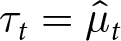 $\tau _{t}=\hat{\mu}_{t}$ and
 $\tau _{t}^{z}=\tau
_{t}^{\ell }=\tau _{t}^{r}=0$.
First, combining equations (31) and (33) from the competitive equilibrium yields
 \begin{equation}
F_{t,n}^{\prime }=f_{3t,n}^{\prime }(p_{3,t}+\tau _{t}^{r}).
\end{equation}
Comparing it with equation (16) from the system that characterises the socially optimal allocation, we get
 \begin{equation}
p_{3,t}+\tau _{t}^{r}=F_{t,E_{3}}^{\prime },
\end{equation}
and from (31) 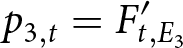 $p_{3,t}=F_{t,E_{3}}^{\prime }$ so we prove that
 \begin{equation}
\tau _{t}^{r}=0.
\end{equation}
Second, combining equations (31) and (34) yields
 \begin{equation}
F_{t,n}^{\prime }=f_{4t,n}^{\prime }(p_{t}^{z}+\tau _{t}^{z}).
\end{equation}
Comparing it with equation (17), we get
 \begin{equation}
p_{t}^{z}+\tau _{t}^{z}=\hat{\mu}_{t},
\end{equation}
and for (35) we know 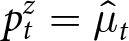 $p_{t}^{z}=\hat{\mu}_{t}$ so we prove that
 \begin{equation}
\tau _{t}^{z}=0.
\end{equation}
Finally, comparing equations (22) and (41), we get
 \begin{equation}
\hat{\mu}_{t}=\tau _{t}+\tau _{t}^{\ell },
\end{equation}
and with 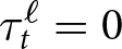 $\tau _{t}^{\ell }=0$ we get
 \begin{equation}
\hat{\mu}_{t}=\tau _{t}.
\end{equation}
This completes the proof of Proposition 3.2.
Proof of Corollary 3.3
It follows from Proposition 3.2 that 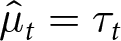 $\hat{\mu}_{t}=\tau _{t}$. Combining this result with equation (35) derived from the first-order conditions of the problem in the oil and coal sectors, we get that the price of carbon capture,
 $p_{t}^{z}$ – technological and from carbon sinks – equals the social cost of carbon,
 $
\hat{\mu}_{t}$, which is Corollary 3.3:
 \begin{equation*}
p_{t}^{z}=\hat{\mu}_{t}.
\end{equation*}




