

1 Introduction
This paper investigates fiscal sustainability in an overlapping generations economy with endogenous growth coming from human capital formation through educational spending. In the model, the government is allowed to run budgetary imbalances that can lead to the emission of public debt. Excessive accumulation of public debt can lead to a collapse of the economy by fully crowding out physical capital. A policy is said to be sustainableFootnote 1 if the corresponding intertemporal economic equilibrium exists. The objective is to assess how budgetary imbalances affect economic dynamics and the outlook for economic growth, thereby providing a rationale for fiscal rules ensuring sustainability, and to analyze the macroeconomic and budgetary implications of Europe's population ageing.
The tax and transfer system examined in this paper is fairly rich. Pension benefits are assumed to be paid in a lump-sum manner. Individuals pay a proportional tax on labor income and at the same time they either pay a lump-sum tax or receive a lump-sum transfer. Labor income taxation is characterized by high top marginal tax rates and relatively lower average effective tax rates, reflecting the progressiveness of income taxation. This is well captured in our model by combining a proportional income tax with a lump-sum transfer. In addition to the tax-benefit system, the government finances general public spending – which benefits individuals but does not distort their economic decisions – and issues bonds. As individuals maximize utility and therefore react to fiscal policy, the model provides a suitable framework to inquire about fiscal sustainability.
There is a large and growing literature on the convenience of imposing fiscal rules, as well as on their desirable properties in terms of sustainability and stabilization. Fiscal rules are in general justified as a way to prevent governments from choosing levels of taxation or spending that do not maximize social welfare because of political biases (see, for example, Alesina and Perotti, Reference Alesina and Perotti1995; or Milesi-Ferretti, Reference Milesi-Ferretti2004). Political biases in fiscal policies can ultimately lead to increasing debt ratios, possibly endangering fiscal sustainability. In dynamic models, where absence of control of the debt dynamics may endanger sustainability, fiscal rules can help stabilize the dynamics of an economy that would otherwise be inherently unstable by maintaining the economy on a sustainable path.
Overlapping generations models are suitable theoretical tools to address fiscal sustainability issues. First, fiscal policy has real effects on the economy (no Ricardian equivalence). Second, since debt dynamics are in general unstable, fiscal rules are needed to maintain fiscal sustainability. In the classical Diamond model (Diamond, Reference Diamond1965), where the only source of economic growth is the accumulation of physical capital, De la Croix and Michel (Reference De la Croix and Michel2002) and Rankin and Roffia (Reference Rankin and Roffia2003) define and study fiscal sustainability. We extend here their analysis to an endogenous growth model in which the interest rate and the growth rate of the economy are jointly determined. There are two sources of economic growth in our model: the accumulation of physical capital and the formation of human capital. The accumulation of physical capital stems from individual savings. Endogenous growth results from the formation of human capital, which is assumed to result from parental education and educational spending, financed out of altruism. The human capital part of the model includes another channel through which government debt affects the economy. Not only is physical capital crowded out by government debt but human capital as well, so that the growth potential of the economy is affected. In other words, not only is the steady state level of capital altered, as it is in existing exogenous growth models, but also the growth rate.
The main findings are the following. First, the existence of steady states is not sufficient to ensure fiscal sustainability. Second, in the presence of multiple steady states, the initial conditions in the economy matter for the long-run equilibrium that will result from economic dynamics. Third, the stability properties of the economy depend on the set of fiscal instruments, i.e., on the adopted fiscal rules. Fiscal policy rules are generally needed to ensure the stability of equilibria that are dynamically efficient. In the literature dealing with public debt, two sorts of fiscal policy rules have in general been assumed:Footnote 2 the constant debt policy and the constant deficit policy. We will however concentrate on the former policy (to be precise, a constant debt to GDP ratio policy), since its implementation is much easier in our model and our main objective is to illustrate how rules change the dynamics of the economy (for a comparison of suggested and currently implemented operational rules, see Buiter, Reference Buiter2003).
The appropriate response of fiscal policy to exogenous temporary shocks is not trivial in the absence of fiscal rules. If temporary small shocks occur in the neighborhood of a stable steady state, there is no strong case for adjustments to fiscal policy, as the economy can come back to its initial position by itself. However, when temporary shocks occur in the neighborhood of an unstable steady state, which is the standard case in an economy with public debt, they endanger fiscal sustainability. Without timely reaction to such shocks, ensuring fiscal sustainability would require adjustment, possibly of a disruptive nature, in the future: the more the adjustment is delayed, the larger its necessary scale is. Fiscal rules preserving fiscal sustainability seem more appropriate to deal with small shocks, as they timely maintain the economy on a sustainable path and do not lead to disruptive adjustments.
We illustrate this point by performing a rough simulation in which a baseline version of our model, parameterized to fit the values of economic variables in the pre-enlargement European Union, is exposed to a demographic shock. To be precise, we assume that the projected decrease in population happens in the next 50 years and show how this can lead to unsustainable debt unless a fiscal rule is introduced.
The paper is organized as follows. In Section 2 we present the main assumptions of our model. In Section 3, the dynamics of the state variables (human capital, physical capital, and public debt) are discussed. In Section 4, we introduce a simulation exercise, parameterizing a baseline version of the model and analyzing its properties. Finally, as an illustration, we assess how this baseline would react to a demographic shock similar to the one the European Union is expected to suffer in the next 50 years. Section 5 concludes the paper.
2 Model
The basic framework is an overlapping generations model (Allais, Reference Allais1947; Samuelson, Reference Samuelson1958; Diamond, Reference Diamond1965), in which parents have an altruistic concern for their children. Parents choose educational spending so as to maximize the expected net labor income of their children.Footnote 3 They are therefore aware that the return to education is affected by labor income taxation. The tax system is fairly rich and encompasses both proportional and lump-sum labor taxes as well as old-age benefits. We consider both the case of balanced budget policies, whereby taxes levied on labor finance old-age benefits so that the tax system functions as a pay-as-you-go public pension scheme, and the case of public debt, whereby the government can run budget deficits or surpluses.
2.1 Households
The economy consists of a sequence of individuals who live for three periods: childhood, adulthood, and old-age. In the second period of their life, each individual gives birth to 1+n t children, which is also the population growth rate when n t=n t−1

where N t denotes the number of individuals born in period t−1.
Individuals are educated during childhood and their human capital during adulthood mainly depends on their parents' educational spending and on their parents' human capital according to

where e t and h t are parental spending on education and parents' human capital, respectively, while F t denotes economy-wide technological progress in the field of education. δ∊(0, 1) stands for the elasticity of human capital with respect to private educational spending. Though education policies together with individual decisions clearly affect human capital formation, we do not address this issue in this paper, where technological progress in human capital formation is assumed to be exogenous.
During adulthood each individual born at t−1 supplies inelastically h t efficiency units of labor, receives a gross labor income w th t, pays proportional (τt) and lump-sum (ηt) taxes, consumes c t, saves s t, and spends (1+n t)e t on education

where ωt stands for labor income net of taxes. When old individuals consume the proceeds of their saving (R t+1s t), along with their lump-sum pension benefits (Θt+1)

where d t+1 denotes old-age consumption.
We assume that parents finance their children's education out of altruism.Footnote 4 They choose educational spending so as to maximize the net labor income of their children. There is no bequest motive in the model. The inclusion of bequests would allow parents to exercise their altruism in two different ways: through education or bequests. Depending on how they are modeled, operative bequests may lead to debt neutrality and consequently to the absence of real effects of fiscal policy when taxes and public transfers are lump-sum (see Lambrecht et al., Reference Lambrecht, Michel and Vidal2005). As our aim is to examine government debt in a model where fiscal policy is effective and there are risks to fiscal sustainability, we assume that there are no bequests.
Each individual born at time t−1 is endowed with the following utility function

where 0<β<1 is a discount factor and γ>0 is the degree of intergenerational altruism. g t denotes the consumption of public goods in period t; as the utility is separable, the provision of public goods does not affect the first-order conditions. The net labor income of children is

Individuals maximize (4) under their budget constraints (2)–(3) and (5). The first-order conditions of an individual's maximization problem are
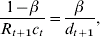

Equation (6) determines consumptions over the life-cycle: the marginal rate of substitution between adult and old-age consumption is equal to the rate of interest. Equation (7) determines parental educational choices. The utility loss in terms of reduced consumption of spending one euro on children's education is equal to the utility gain stemming from the increase in children's income out of altruism. Merging equations (2) and (3) gives an individual's life-cycle budget constraint

where W t denotes life-cycle disposable income.
There is no intragenerational inequality, as all individuals belonging to the same cohort are identical. The tax system only entails intergenerational redistribution. In an endogenous growth model, lump-sum transfers can be linked to a growing variable. We here assume that they are related to labor income at the aggregate levelFootnote 5

Life-cycle disposable income is therefore given by

T t indicates the implicit tax rate paid on labor income over the life cycle. This tax rate is positive if the rate of interest is higher than the implicit rate of return on public pensions:  .
Combining the life-cycle budget constraint (8) with condition (6), we can write


Plugging the expression for c t into condition (7), we obtain an equation characterizing the optimal choice of educational spending

Together with (9), equation (11) gives the optimal education spending

The optimal consumption and saving can therefore be expressed as follows


where we define

Equation (15) relates savings to wage income. The savings ratio depends on fiscal policy parameters and on the expected interest rate.
2.2 Firms
In each period t, production occurs according to a Cobb–Douglas technology using two inputs: physical and human capital. Output is given by

where K t and H t denote the levels of physical and human capital in period t, respectively. A t is a technology parameter, indicating exogenous technological progress over time, and α∊(0, 1) is the share of physical capital.
The stock of capital in period t (K t) comes from the total savings of the preceding period, public or private. The demand for labor (effective labor or human capital) maximizes profits

The resulting wage is the competitive one

The remaining profits belong to capital owners so that we can define the return on physical capital as

2.3 Public sector
In each period, the government levies income taxes  and pays pension benefits to retirees (θtw t−1H t−1), finances public consumption G t=(N t−1+ N t−2)g t, reimburses the outstanding public debt Bt−1 along with the accrued interests (R t−1)B t−1 and issues government bonds B t, which will be redeemed one period later. In period t, the government budget constraint is

The relevant statistical concept for public debt in the model at hand is net debt, i.e. the difference between general government's liabilities and assets.
3 Intertemporal equilibrium
3.1 The economic growth rate
Merging equations (1) and (12), we obtain the law of motion of human capital per capita

where

Assuming either that all the exogenous parameters and prices are constant over time, which would be the case for a small open economy, or else that prices have converged to their steady-state levels in the closed economy case, Φ (w, R)−1 is the growth rate of per capita human capital.
Labor supply in period t is equal to the aggregate level of human capital in the economy. The aggregation of the levels of human capital of the N t−1 individuals can be written as: H t=N t−1h t. Using (20) we obtain the growth rate of aggregate human capital: (1+n t)Φt(w t, R t+1)−1.
3.2 Physical capital and public debt
Savings finance both physical capital and public debt, so that the following capital market clearing condition holds

The intertemporal equilibrium in this economy can thus be defined as a sequence {K t+1, B t+1}t=0∞ satisfying the following equations


If the growth rate of aggregate human capital is known, the dynamics of the economy can finally be summarized by a system of two equations expressed in intensive terms


where k t=K t/H t, b t=B t/H t, and  t=G t/H t, and are the ratio of physical to human capital, the ratio of public debt to human capital, and public consumption per unit of human capital in period t, respectively.
It is well known that there are normally two steady-state solutions when we introduce public debt in a standard overlapping generations economy. This is also the case in an endogenous growth model such as the one presented here. The simulations below aim at illustrating the functioning of the system and the consequences of budgetary imbalances in a model calibrated with European data. We subsequently analyze the macroeconomic and budgetary implications of population ageing in Europe.
4 Simulations
In this section, we produce a rough calibration of the model with the objective of providing some examples about how fiscal sustainability can be guaranteed in the presence of diverse shocks. The way to proceed is to calibrate first a baseline scenario, where response to the mentioned shocks will then be assessed.
4.1 Baseline scenario
The calibration of two- or three-period overlapping generations economies is not very usual in the literature. The main difficulty in dealing with this issue is the need to simulate very long time periods. In the current example, we follow De la Croix and Doepke (Reference De la Croix and Doepke2003) in assuming time periods of 30 years; that is, a typical individual lives for 90 years. During the first 30 years (childhood), she just receives education; she works, consumes, and saves during the following 30 years (adulthood); and, finally, she lives out of her retirement pension and savings for the last 30 years (retirement).
Macroeconomic assumptions
The macroeconomic assumptions refer to the choice of the parameters that ensure reasonable interest and growth rates in the baseline scenario. Of course, the final interest and growth rates also depend on public finance assumptions.
The main parameters of the model with their chosen values are shown in the following:
β=0.4252Equivalent to a yearly discount rate of 0.99
γ=0.169From De la Croix and Doepke (Reference De la Croix and Doepke2004)
δ=0.6From De la Croix and Doepke (Reference De la Croix and Doepke2003)
α=0.3Standard range in the literature
For the particular choice of utility function selected in this model, β represents the weight of old-age consumption in the utility of each individual. The value chosen is equivalent to a yearly discount factor of 0.99. This is higher than the usual estimate of 0.96 more frequently used in the literature. The qualitative conclusions of the model are the same with both values but this higher β allows us to produce more reasonable interest rates. γ is an important parameter in this model since it represents the degree of altruism that ultimately leads parents to worry about their children's education. The value of 0.169 is taken from De la Croix and Doepke (Reference De la Croix and Doepke2004). They give an alternative value of 0.271 in De la Croix and Doepke (Reference De la Croix and Doepke2003) but the first one is preferred for the same reasons expressed in the choice of β. The same source is used for the choice of 0.6 as the value for δ, the elasticity of human capital with respect to educational spending. The value of the capital share (α=0.3) is taken in the usual range employed in the literature. The values chosen for the technology parameters A and F, which are just scale parameters, are respectively 50 and 1.05.
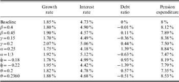
The population growth rate assumed is 0.34% per year. This represents European Union population growth during the 1990s (EUROSTAT 2002 Yearbook). This population growth and technology parameters, together with the fiscal policy explained below give rise to a per capita output growth of 1.85% per year and a yearly long-term interest rate of 4.73%.
Public finance assumptions
The baseline scenario is calibrated for a case in which the budget is balanced every period and there is no net public debt. By zero net public debt, we mean that the government is neither a net lender to, nor a net borrower from, the other sectors of the economy. This does not mean that the government has zero liabilities but that government liabilities are equal to government assets. Net government debt is the relevant concept in the model at hand; it departs from the definition of general government gross debt as the consolidated liabilities of the general government sector, which is usually referred to as headline debt. This calibration is broadly supported by available empirical evidence. The net financial liabilities of general government in the euro area are of an order of magnitude of 50% of GDP (see OECD, 2007: 253). Estimates of the stock of public capital (see Kamps, Reference Kamps2004: 7) are of the same order of magnitude, suggesting that government net debt can be calibrated to zero. The other fiscal policy parameters have been set as follows:
τ=0.6Marginal tax rate
 Consistent with an effective tax rate on labor income of 40%
θ=0.2196Consistent with a pension expenditure ratio over GDP of 8%
- =17.6228Consistent with public consumption of 20% of GDP
The marginal tax rate on labor income (τ) and the lump-sum tax/transfer ( ) have been chosen with a view to replicating both the effective tax rate and the high marginal tax wedge on labor income in the European Union. The marginal tax rate set at 60% (τ=0.6) captures the high marginal tax wedge on labor income in the European Union, where progressiveness in the statutory tax rates on personal income is moderated by a wide range of tax allowances and tax credits and the proportionality of social contributions (Joumard, Reference Joumard2002). Martinez-Mongay (Reference Marín2000) indicates that the effective tax burden on labor in the euro area was close to 40% in 1999, slightly higher than the effective tax burden in the European Union. These estimates are corroborated by those calculated by Mendoza et al. (Reference Mendoza, Razin and Tesar1994) for Germany, France, Italy, and the United Kingdom. The difference between the European Union and the euro area is attributable to the low effective tax rate on labor in the United Kingdom (about 25%). The choice of the lump-sum transfer (
 ) is driven by the estimates for the effective tax burden on labor (
 ). Alternatively, this calibration can be justified by the fact that taxes (13%) plus social contributions (15%) represent 28% of the European Union's GDP for the period 1995–2000 (EUROSTAT 2002 Yearbook).Footnote 6 Knowing this and given the assumption of a Cobb–Douglas production function, we can calculate


As for the pension parameter (θ=0.2196), its value has been generated endogenously from the choice of all the rest of the parameters, which have been chosen to obtain a pension expenditure to GDP ratio of 8%. This ratio was the actual number for the pre-enlargement European Union in 2000. Under budget balance, we have

We can then compute the pension expenditure to GDP ratio

Finally, =17.6228 is chosen so as to fix  , which is the value of government consumption in the pre-enlargement European Union in the period 1995–2000.
In an alternative scenario, choosing β=0.2308 (0.96 yearly discount rate), γ=0.271 and α=1/3, and with fiscal policy parameters  and θ=0.2360 (which ensure again that the pension expenditure ratio over GDP is 8%), we generate a per capita output growth of 1.93% per year and a yearly interest rate of 7.88%.
Calibrating a two- or three-period overlapping generations model is a delicate exercise: the limited number of parameters leaves relatively little room for maneuver, possibly making the baseline calibration highly sensitive to change in assumptions. The sensitivity of our baseline calibration to changes in parameters can be observed in Table 1, in which only one parameter differs from the baseline scenario in each variant.
Sensitivity of baseline calibration to changes in parameters

Steady states: existence and stability
Existence of steady states
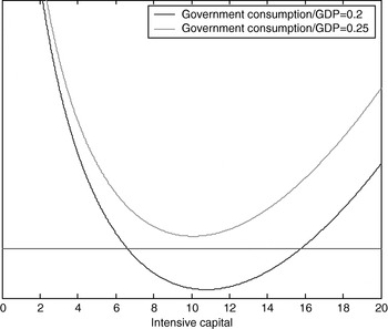
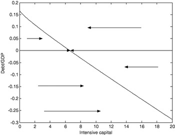
The existence and characterization of steady states depend critically on the assumptions about the fiscal policy that the government is implementing. First of all, let us assume that the government fixes taxes and pension benefits, as well as government consumption as a fraction of GDP and lets the economy work by itself. The dynamics of such an economy would be governed by the dynamic system defined by equations (22) and (23). The first question is whether or not such an economy will converge to some steady state. To study this, we can fix all the parameters and assume k t+1=k t=k and b t+1=b t=b in these two equations. We can then easily obtain a single non-linear equation in k, which is represented in Figure 1.
Steady state of the baseline calibration

The intersection of the black line and the x-axis represents the set of steady states for the baseline calibration. There are two steady states resulting from this choice of parameter values. The existence of steady states is fragile and crucially depends on fiscal policy. For example, increasing government consumption from 20% to 25% of GDP is sufficient to disrupt the long-term economic equilibrium, as can be seen from Figure 1. Similar results can stem from excessive public expenditure ratios and either excessive or insufficient taxation. With our specification of the economy, steady states are multiple (two), unless they do not exist, except for the special case of a tangency solution. From these two steady states, the first one is associated with dynamic efficiency (under-accumulation of capital), while the second is in general in the area of dynamic inefficiency.
Stability analysis and selection of a policy-relevant steady state
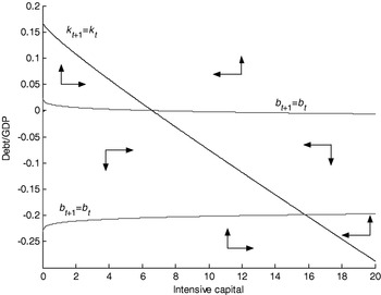
The dynamics of the system can better be observed in the following phase diagram, which corresponds to the baseline calibration (see Figure 2). First, the two steady states identified by Figure 1 are located at the intersection of the curves k t+1=k t and b t+1=b t. Second, we can observe what the associated net debt to GDP ratio is for each of the two steady states: zero for the first steady state (it was calibrated for this to be the case) and a net lending position of 19.89% of GDP for the second.
Phase diagram of the baseline calibration

It can be seen from the diagram that the first steady state is stable in the saddle path sense, with a saddle path slightly decreasing in the net debt ratio in the proximity of the steady state.
This means that, for any initial intensive capital value, there is only one debt level that would lead the economy to this first steady state, characterized by under-accumulation of capital. Debt, however, is a stock variable and there is no mechanism in this economy that can set the debt ratio on the saddle path so that a small perturbation will lead the economy to diverge from the steady state. We can notice that if the perturbation leads to a debt level below the saddle path, the economy, evolving according to its own law of motion, will converge to the second steady state. However, if the perturbation leads to a higher debt level, the economy will inexorably diverge to reach a zero capital level, unless some kind of discretionary fiscal policy is adopted or new countervailing shocks happen.
As for the second steady state, it is situated to the right of the golden rule intensive capital level. The golden rule intensive capital level is defined as the solution to the equation

For the baseline calibration, this value is 14.5925, which is lower than the second steady state, situated at a level of intensive capital of 15.8052. At this steady state, thus, the economy is in an area of dynamic inefficiency, as defined in Cass (Reference Cass1965). The growth rate of the economy (in per capita terms) at this steady state is 2.53% per year with a yearly real interest rate of 2.62%. The pension expenditure ratio amounts to 6.57% of GDP.
Why is this stable steady state not considered so carefully? The reason, in addition to the fact that it is associated with an unusually high net lending position of general government, is the number of studies that have established how extraordinary is that an economy is in a dynamically inefficient steady state (Mankiw et al., Reference Mankiw, Romer and Weil1992). It must be noticed, though, that this steady state is robust to small perturbations. Even more, it can be said that once the economy is in this steady state, an unreasonably big shock is required to endanger fiscal sustainability, as the government is a net lender to the economy. Another justification for not concentrating on the study of the over-accumulation steady state is based on political economy arguments. Once governments start running budget surpluses, it is very unlikely that they will keep the same budget policy instead of spending their extra resources. A good example of this can be found in the United States debate about what to do with the fiscal surplus at the end of the 1990s.
Unsustainable debt dynamics
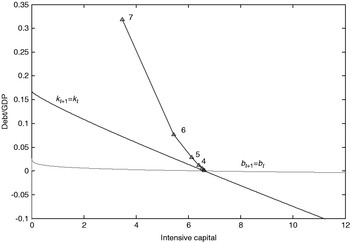
Coming back to the first steady state, theory tells us that it is inherently unstable, making fiscal sustainability very fragile. Suppose that the economy situates itself with a slightly higher debt to GDP ratio than that implied by the steady state. An example can be seen in Figure 3. The initial conditions are set at the under-accumulation steady state plus some arbitrary small amount of additional government liabilities (0.1% of GDP). Such a small perturbation (we can make it arbitrarily small) is sufficient to disequilibrate the system. If the same fiscal parameters are nevertheless kept, public debt starts to accumulate, very slightly in the first periods but at an increasing rate. In this example, the economy would crash at the eighth period. Remember that this is a discrete time model so that we have jumps in the phase diagram; the jump after the seventh period would lead us to negative capital levels, that is a collapse of the economy.
Trajectory of the baseline economy starting from steady state

Fiscal rules ensuring sustainable debt dynamics
It could be argued that this should not be a major concern since eight periods in this model represent actually 240 years. It is true that it is very extreme to assume that nothing else would change in 240 years, although some civilizations may have collapsed as a result of fiscal problems in such a time span. However, the best way to reconcile this model with the behavior of real economies is to think that the economy is never in the steady state and that the phase diagram is continuously changing, as the long-run steady state also depends on fiscal policy decisions. In this case, fiscal sustainability can be a more delicate issue than the previous numerical analysis would suggest, since the instability of the system, and hence the risks of a sustainability crisis, greatly multiplies when the economy is far from the steady state.
Is there any way to limit this intrinsic instability of the first steady state? The government can proceed in two different ways in this setup. One solution is to adopt discretionary policies only after significant budgetary imbalances have accumulated. For example, the pension system can be extremely generous during one generation putting the economy on an explosive path but then policies can change so as to approximate a new steady state.
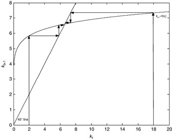
A more systematic solution would come from adopting a fiscal rule maintaining the economy on a sustainable path. The adoption of a fiscal rule changes the dynamics of the system. The fiscal rule that will be considered in this paper is that of a fixed net debt policy. Suppose then that the government fixes a desired net debt ratio and adjusts its fiscal policy instruments. In the ensuing simulations, we will keep fixed the tax parameters and will use either the pension benefits (θt) or government consumption (G t) as equilibrating variables. In either case, the dynamics of the system will be described by Figure 4, which has been drawn for the case in which the targeted net debt ratio is 0 (budget balance). The steady state is unique here and it is globally stable, as we know is the case in general whenever we have budget balance. We obtain the same result for all feasible debt ratios. The set of feasible debt targets under a fixed debt policy and their associated intensive capital values are depicted in Figure 5. Any policy aiming at sustaining a debt level over the depicted line would lead the economy to a negative capital stock or, in other words, would not be sustainable.Footnote 7
Capital dynamics for a fixed debt policy (b=0)

Dynamics of different fixed debt policies

The costs of delaying fiscal adjustment
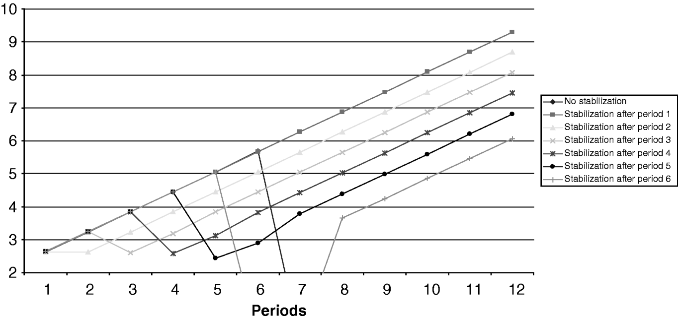
There are of course intermediate solutions between the two extremes of keeping the same fiscal structure (Figure 3) or adopting a fiscal rule (Figure 4 or 5). On the theory side (see for example Schmitt-Grohe and Uribe, Reference Schmitt-Grohe and Uribe2004), fiscal rules usually set the tax revenue as an increasing function of government liabilities. The adjustment speed of this function to some target level is then chosen by the government so as to minimize some kind of loss function or, equivalently, to maximize national welfare. Studying optimal fiscal policy or even the optimal fiscal rule goes beyond the scope of this paper, but the effect of alternative policy scenarios can be appreciated through the following experiment. Take the example of Figure 3 in which the economy starts from the steady state capital level but with a small amount of public debt equivalent to 0.1% of GDP. Now suppose that instead of not reacting to the fiscal crisis, the government decides to revert to a fiscal rule (one implying zero debt in this case) at some point in time. Figure 6 shows the effects of this policy on the average utilityFootnote 8 level depending on when the government decides to recourse to the fiscal rule. The costs of delaying the response to fiscal problems are reflected in a high cost of fiscal stabilization during the period in which the economy reverts to the rule and in the fact that the economy settles in a lower path of growth after stabilization than the one that would have been attained if the stabilization policy had been undertaken in time.
Average utility
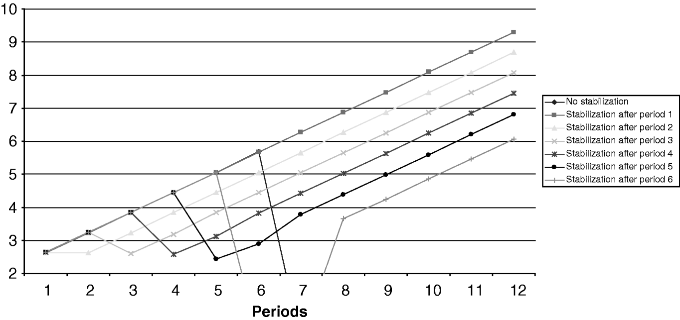
In this experiment, the way in which fiscal stabilization is obtained is by reducing the level of public expenditure so as to go back to a level of zero public debt. As a result, an indirect measure of the cost of fiscal stabilization at different points in time is given by the reduction of the percentage of public expenditure over GDP that has to be given up in order to achieve it at different points in time. For example, suppose that the government decides to ‘stabilize’ after period 1 in which the level of public debt has been of 0.1% of GDP. In that case, public expenditure needs to go from 20% of GDP to 19.77% in period 2 (it immediately goes back to 20% again in period 3 once the stabilization has been obtained). If ‘stabilization’ takes place after period 2, public expenditure needs to be reduced to 19.48% of GDP for one period. After period 3, the number would be 18.80% of GDP. After period 4, we would need to reduce public expenditure to 17.14% of GDP. After period 5, the reduction would have to go till 12.36% of GDP. Finally, for ‘stabilization’ to take place after period 6, a negative public expenditure ratio would be required (−11.84% of GDP), which amounts to say that going back to a zero public debt level in one period would be impossible just by reducing the level of public expenditure and either other measures (reducing pension benefits) or more gradual policies would be required.
Another way of stabilizing would be to choose a different debt target after the shock takes place. Suppose that the government decides to stabilize at a debt-to-GDP ratio of 0.1% once the shock takes place. In the end, this is a matter of intergenerational redistribution. The brunt of the cost will come in the period in which stabilization is decided. Setting a higher debt target would imply a lower capital steady state that would be reflected in lower growth rates and lower utility for the rest of the periods.
4.2 Fiscal sustainability and population ageing
The issue of fiscal sustainability has become increasingly popular in Europe in relation to the possibility or impossibility of keeping unchanged the public pension arrangements in view of the estimates of population decrease over the next 50 years. We will analyze what the prediction of our model for this particular case is.
The demographic shock consists of a change in the population growth rate. The EPC-Budgetary challenges posed by population ageing projects (Section 2.2) that the total population of the European Union (before enlargement) will go from 376.4 million in 2000 to 364.2 million in 2050. This gives us a yearly population decrease of 0.07% per year that we must compare to the yearly population growth of 0.34% assumed in the baseline scenario. The way we introduce the shock is by assuming that −0.07% will be the generation growth rate after two periods (in the new steady state), that is n t+2=(1–0.0007)30. The transition is modeled by choosing n t+1 so that the total population after two periods is  times that of the baseline.Footnote 9
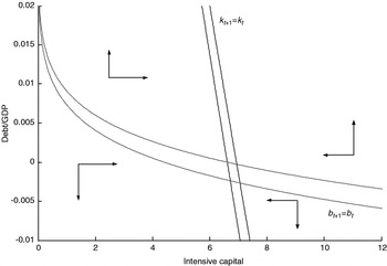
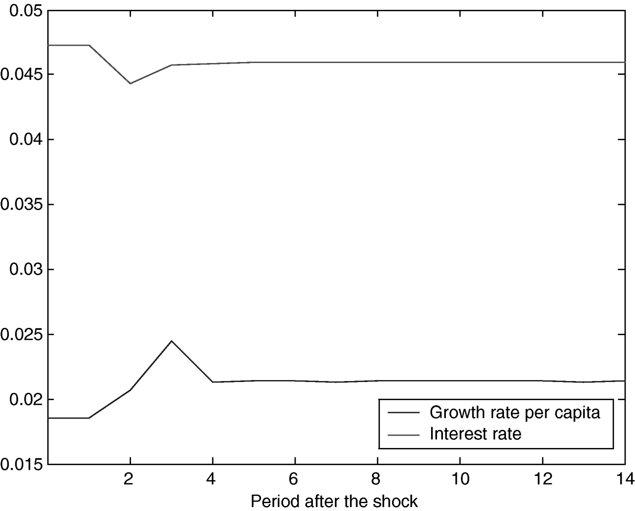
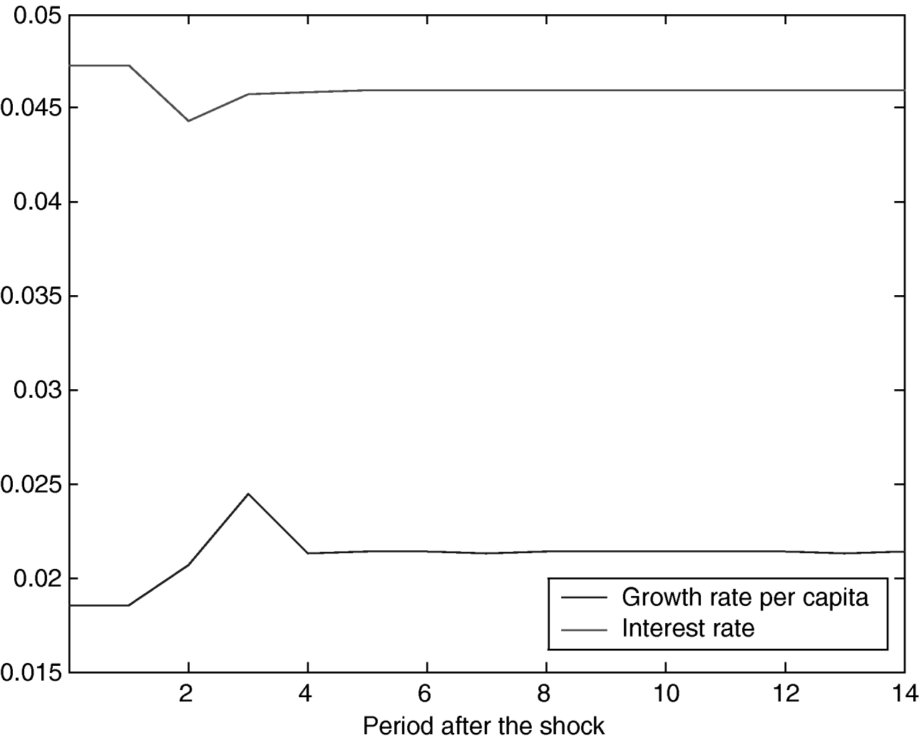
Figure 7 compares the baseline with the new dynamic system around the dynamically efficient steady state. We can see that the new steady state is characterized by higher intensive capital level and a net government debt of −0.27%. The per capita growth rate associated with the new steady state would be 2.15% (compared with 1.85% in the baseline) and the interest rate 4.57% (compared with 4.73%). Keeping the same policy parameters, the pension expenditure ratio would increase to 8.28% of GDP (0.28% of GDP higher than the baseline).
Phase diagram after a demographic shock (from 0.34% to −0.07% yearly population increase)

The reason why the new steady state features higher growth comes from the structure of the model. Growth is generated by investment in human capital. A lower population growth rate allows each parent to invest more in each of the remaining children so that they will have a higher per capita human capital that will show up as a general higher growth rate in all the relevant variables in the economy.
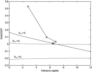
Importantly, it is misleading and dangerous to compare directly two steady states. By looking at Figure 7, we can realize that the economy would not go to the new steady state. In fact, we can run a simulation to see what would happen if policy parameters remain unchanged. The result can be seen in Figure 8, illustrating how the economy would crash five periods after the population shock happens under no policy changes.
Dynamics in a no-change of policy scenario

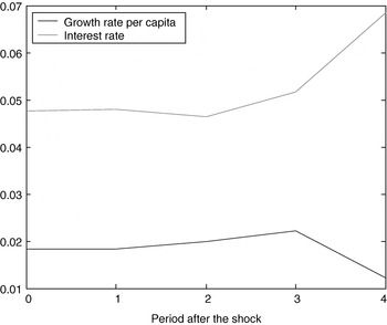
It could be of interest seeing the evolution of some significant variables in the economy along the dynamic path. This can be observed in Figures 9, 10, 11, and 12. It is remarkable that the effect on the interest and growth rate is not really alarming at any point and it is very difficult to deduce that the economy is heading to a disaster. In this respect, neither growth nor the interest rate seems to be a useful indicator of fiscal sustainability by itself.
Effects of the demographic shock

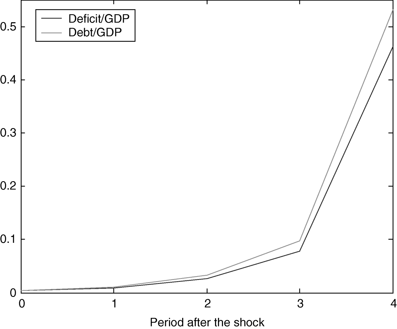
Effects of the demographic shock

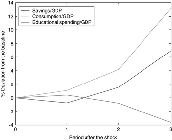
Effects of the demographic shock

Effects of the demographic shock on pension expenditure over GDP

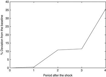
The picture is different if we concentrate on other variables. For example, the behavior of debt and deficit is clearly explosive (Figure 10). Figure 11 shows that the main ratios in the economy: consumption to GDP (around 62.7% in the baseline), savings to GDP (14.4% in the baseline) and private education to GDP (2.9%) also react importantly to demographic shock. Finally, the ratio of pension expenditure to GDP also increases along the dynamics caused by the shock (Figure 12).
We discussed in the previous section that fiscal rules could prevent the economy from entering into unsustainable dynamics. In this case, we will first analyze what is the effect of adopting a fiscal rule of budget balance (zero net debt). When we want to impose budget balance or any other fixed debt policy, we can use either government consumption or pension benefits as equilibrating variables. If we use the latter (pension reform), most of the relevant variables in the economy stay unchanged (the ratios presented in the previous charts). There are of course repercussions on the growth rate per capita and interest rate that can be observed in Figure 13.
Effect of the demographic shock under budget balance
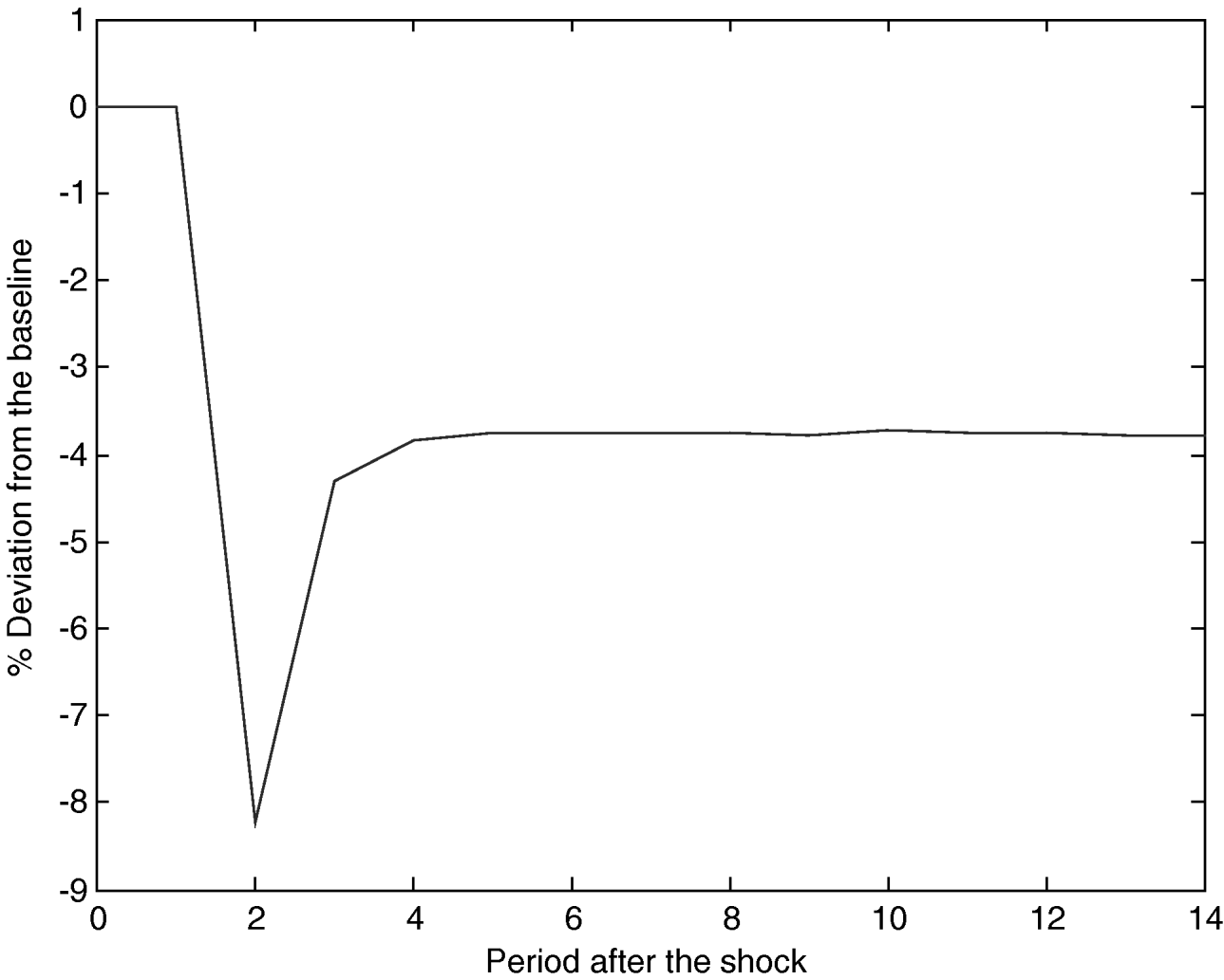
The change in the pension benefits does not affect the pension expenditure to GDP ratio, but it is nevertheless interesting to know by how much pension benefits have to decrease to attain budget balance. This calculation is presented in Figure 14. Benefits can remain unchanged for the first period but must be reduced by more than 8% in the following one. Once the economy stabilizes in the new steady state, benefits can be upgraded slightly but would remain 4% below their original level in spite of the higher growth rate associated with the new steady state.
Evolution of social security benefits after the shock to equilibrate the budget

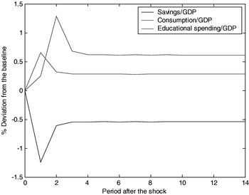
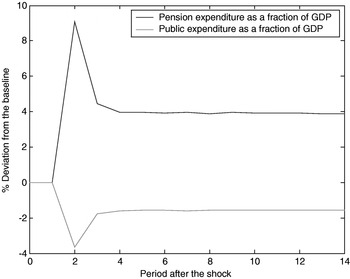
Another possibility for the government to ensure budget balance is to reduce government consumption, while maintaining pension benefits. The effect is exactly the same as was observed in Figure 13 for the interest and growth rates per capita. However, the reaction of other macroeconomic variables is different, as can be seen in Figures 15 and 16. Figure 15 shows that the consumption to GDP ratio increases by 0.6% in the new steady state with respect to the baseline, whereas the savings ratio goes down by some 0.5% of GDP and educational spending with respect to GDP also increases by 0.28%. In Figure 16, we can see how the pension expenditure to GDP ratio evolves when we keep benefits unchanged. It increases by 3.9% of GDP with respect to the baseline in the new steady state. Finally, the necessary reaction of government consumption to equilibrate the economy implies a decrease by 1.6% of GDP.
Effect of the demographic shock under budget balance

Effect of the demographic shock under budget balance

5 Conclusion
The objective of this paper was to analyze fiscal sustainability in an overlapping generations economy in which government imbalances are allowed. The conclusions that can be drawn from this study are the following.
First, it is not sufficient to concentrate on steady state analysis. Fiscal policy is sustainable if the economic equilibrium exists in all periods. This is a general obvious point that we want to make here because of its particular relevance in this model. Importantly, in the demographic shock studied in this paper, it is clear that the new steady state is characterized by higher growth rates and lower interest rates than the one before the shock. However, the economy, led by its own dynamics without any change in fiscal policy, would never attain the new more favorable steady state, but would instead be led to an unsustainable situation.
Second, it must be emphasized that fiscal sustainability can be extremely fragile. All the indicators in an economy may remain at ‘normal’ levels, while the economy is actually in an unsustainable situation.
Third, fiscal policy rules seem to be necessary to ensure fiscal sustainability. The government cannot remain passive in front of the shocks that affect the economy. It must react to those shocks in a way that situates the economy on sustainable paths with a view to preventing the accumulation of significant budgetary imbalances leading to disruptive adjustments. Under fiscal rules, such as a constant debt policy in the framework developed in this paper, the dynamic properties of the economy change and the equilibrium becomes stable.