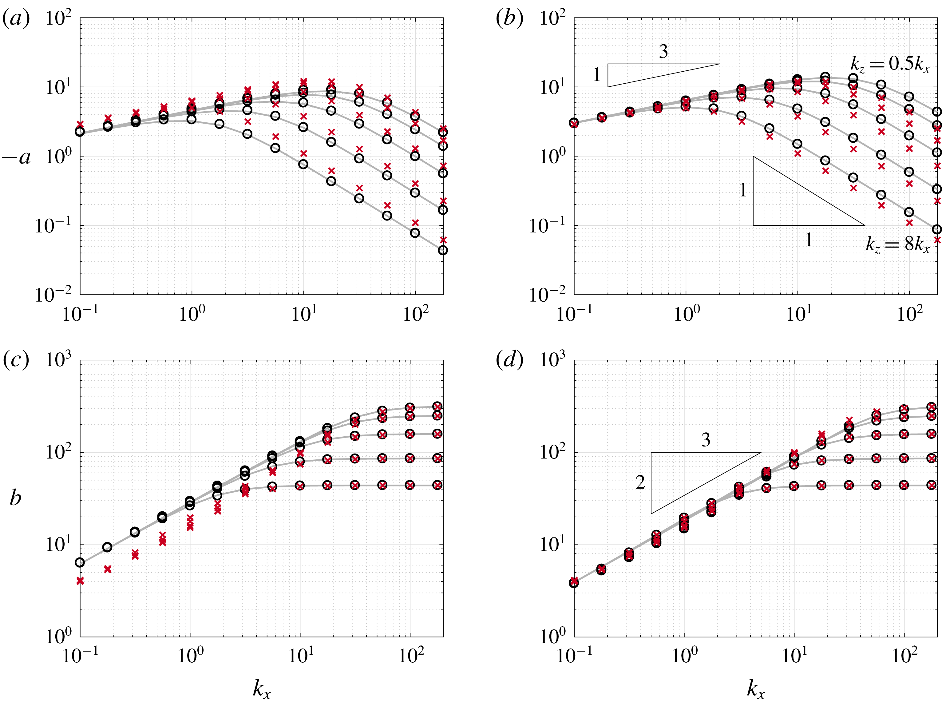
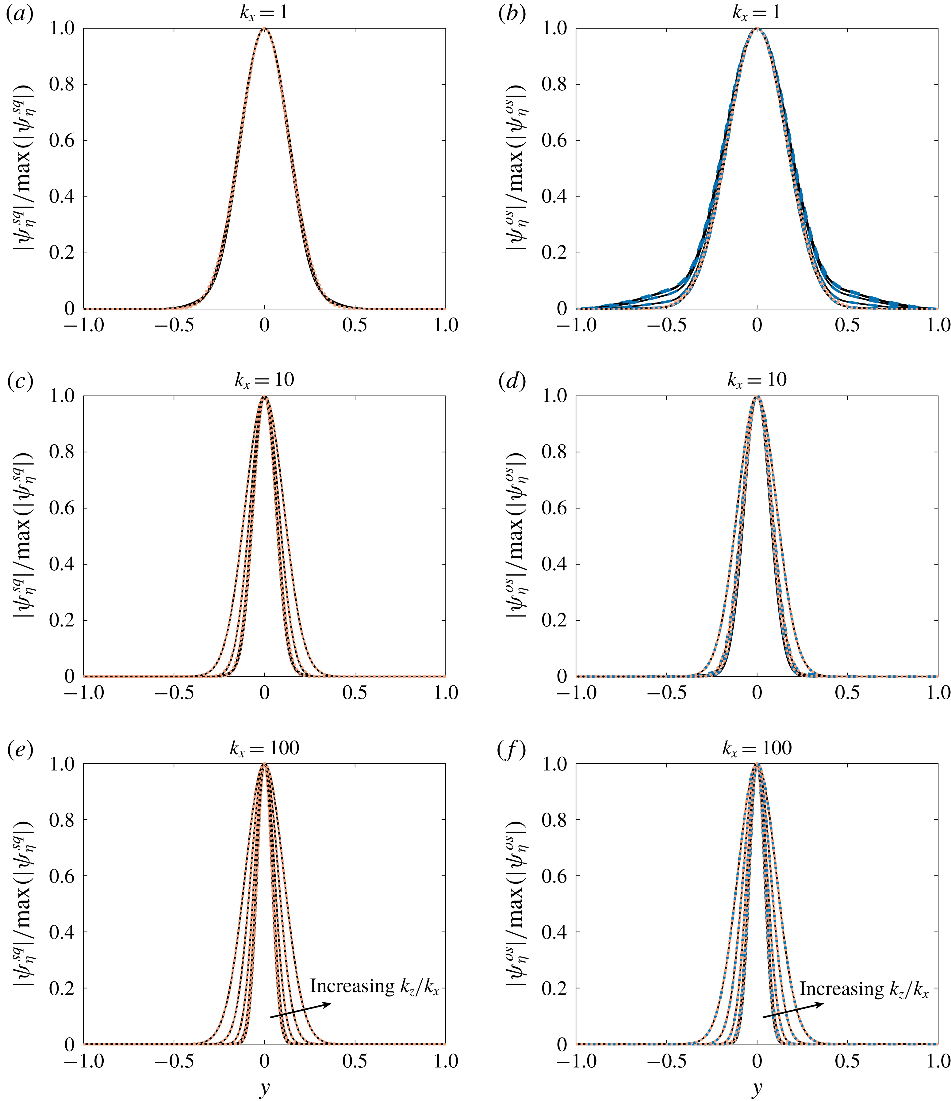
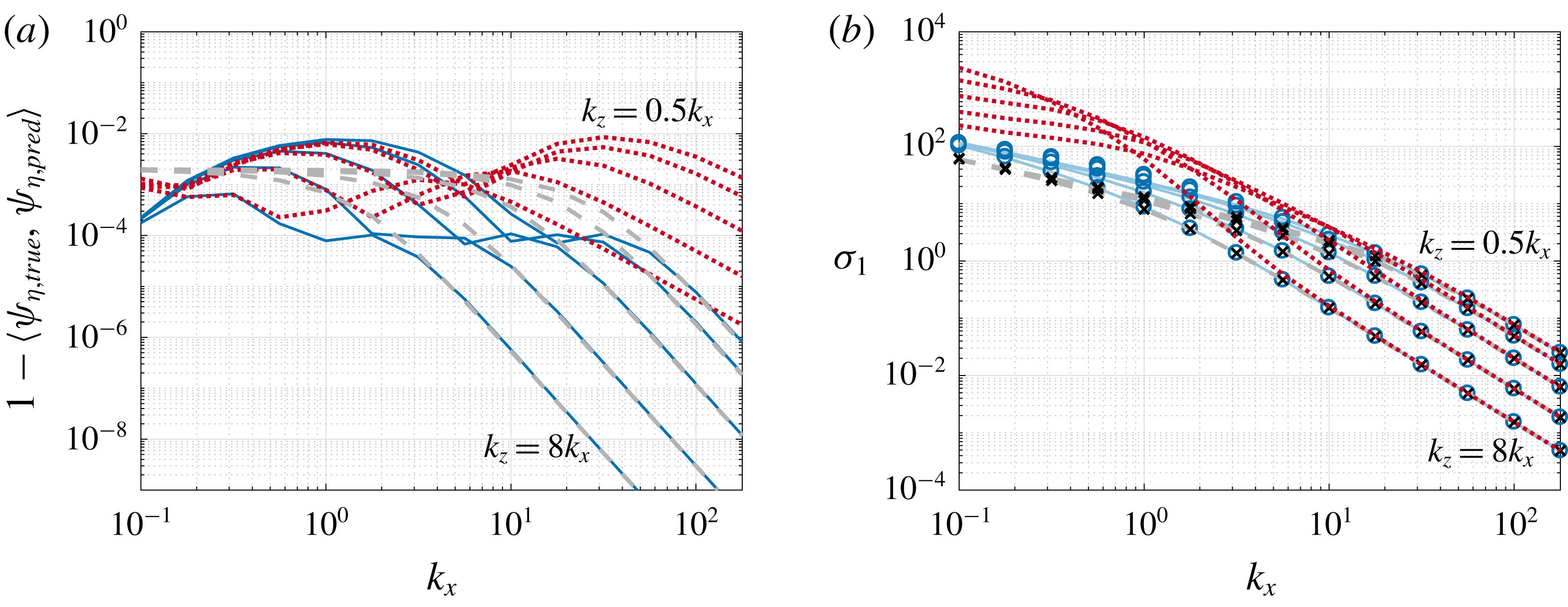
1 Introduction
With the exception of very simple systems, the identification of spatial mode shapes characterising fluid flows typically requires resorting to numerical methods, applied either to discretised (and often linearised) governing equations, or to data collected from experiments or numerical simulations of their evolution. In this work, we describe methods to approximate mode shapes and amplification mechanisms without requiring the formation of discretised operators, for incompressible, quasi-parallel, shear flows.
The identification of pertinent structures that arise in the transition towards, and emerge as coherent features within, turbulent wall-bounded flows has been the focus of much research over the past several decades. Qualitatively, such analysis includes identification and classification of empirically observed structures, such as near-wall streaks (Kline et al. Reference Kline, Reynolds, Schraub and Runstadler1967), hairpin structures (Theodorsen Reference Theodorsen1952; Head & Bandyopadhyay Reference Head and Bandyopadhyay1981) and their grouping in large-scale motions (Zhou et al. Reference Zhou, Adrian, Balachandar and Kendall1999; Guala, Hommema & Adrian Reference Guala, Hommema and Adrian2006), and very large-scale motions or superstructures (Kim & Adrian Reference Kim and Adrian1999; Guala et al. Reference Guala, Hommema and Adrian2006; Hutchins & Marusic Reference Hutchins and Marusic2007). For more details concerning the (sometimes debated) properties, taxonomy and dynamics of such structures, see reviews such as Robinson (Reference Robinson1991), Smits, McKeon & Marusic (Reference Smits, McKeon and Marusic2011) and Jiménez (Reference Jiménez2018), and references within.
On a quantitative level, a starting point for the prediction of coherent structure comes from consideration of properties of the governing equations, most typically in linearised form. Features emergent in wall-bounded turbulent flows often bear little resemblance to modes identified from classical stability analysis (Drazin & Reid Reference Drazin and Reid2004), where two-dimensional modes are predicted to be the least stable by Squire’s theorem, and mean-linearised flows often have only stable eigenvalues (Reynolds & Tiederman Reference Reynolds and Tiederman1967; Del Alamo & Jimenez Reference Del Alamo and Jimenez2006; Cossu, Pujals & Depardon Reference Cossu, Pujals and Depardon2009). Perhaps the most important realisation in the study of such linear operators is the fact that their non-normality can result in high amplification (in either the time or frequency domain), which cannot be predicted from their spectra alone (Böberg & Brösa Reference Böberg and Brösa1988; Butler & Farrell Reference Butler and Farrell1992; Farrell & Ioannou Reference Farrell and Ioannou1993; Reddy & Henningson Reference Reddy and Henningson1993; Trefethen et al. Reference Trefethen, Trefethen, Reddy and Driscoll1993; Schmid & Henningson Reference Schmid and Henningson1994; Bamieh & Dahleh Reference Bamieh and Dahleh2001; Jovanović & Bamieh Reference Jovanović and Bamieh2005; Schmid Reference Schmid2007; Hwang & Cossu Reference Hwang and Cossu2010; McKeon & Sharma Reference McKeon and Sharma2010; Schmid & Henningson Reference Schmid and Henningson2012). Operator non-normality is responsible for both finite-time energy growth of the linear system from a given initial condition, and the amplification resulting from continual forcing (be it stochastic or harmonic). Indeed, these two notions are mathematically related via the Kriess constant of the operator (Schmid Reference Schmid2007).
While most initial works considered laminar base flows, more recent developments have used similar methods for prediction of turbulent features by linearising about states computed from turbulent data and/or models (which are most often mean states). For example, Del Alamo & Jimenez (Reference Del Alamo and Jimenez2006) and Cossu et al. (Reference Cossu, Pujals and Depardon2009) have demonstrated transient growth of near-wall streaks and large-scale motions for turbulent channel and zero-pressure-gradient boundary layers respectively, while Schoppa & Hussain (Reference Schoppa and Hussain2002) has showed that a turbulent mean with the addition of low-speed streaks can give rise to the growth of structures due to secondary growth mechanisms in the near-wall region of turbulent channel flow. The characterisation of the nonlinear Navier–Stokes equations in the frequency domain as the linear resolvent operator acting on the nonlinear ‘forcing’ terms, as developed by McKeon & Sharma (Reference McKeon and Sharma2010) has been particularly fruitful for elucidating operator-based predictions of structure in wall-bounded turbulence, including very-large-scale motions and their scaling (McKeon & Sharma Reference McKeon and Sharma2010), and hairpin structures (Sharma & McKeon Reference Sharma and McKeon2013). McKeon (Reference McKeon2017) summarises further developments in this area.
This work will in particular utilise the formulation in Rosenberg & McKeon (Reference Rosenberg and McKeon2019), where the resolvent formulation of the Navier–Stokes operator is decomposed into Orr–Sommerfeld and Squire components in order to obtain a more efficient representation of exact coherent structures. Here, we use this decomposition to make the application of the techniques that we develop tractable.
While developments in operator-based decompositions for turbulent flows are recent and ongoing, many of the underlying physical mechanisms in shear flows have been understood for at least several decades. These include the Orr mechanism (Orr Reference Orr1907; Jiménez Reference Jiménez2013), which amplifies upstream-leaning disturbances while tilting them towards the downstream direction, and the lift-up mechanism (Landahl Reference Landahl1980, Reference Landahl1975), in which disturbances in the wall-normal direction lead to large streamwise responses. Disturbances that are spatially localised in the streamwise direction can also grow in amplitude as they convect downstream, as is typical for optimal disturbances for systems with streamwise inhomogeneity (Chomaz Reference Chomaz2005; Hack & Moin Reference Hack and Moin2017). Each of these three mechanisms can be related to different aspects of the non-normality of the underlying linear operator (Symon et al. Reference Symon, Rosenberg, Dawson and McKeon2018).
Results concerning the pseudospectral properties of certain matrices (Trefethen & Chapman Reference Trefethen and Chapman2004) and linear differential operators by Trefethen (Reference Trefethen2005) have revealed criteria by which pseudomodes exist that are localised in both space and spatial frequency, and are highly amplified by the associated resolvent operator. This method of analysis has been used, for example, in the analysis of swept wing flow (Obrist & Schmid Reference Obrist and Schmid2010, Reference Obrist and Schmid2011), the stability of the Batchelor vortex (Mao & Sherwin Reference Mao and Sherwin2011) and the study of a trailing vortex wake in Edstrand et al. (Reference Edstrand, Schmid, Taira and Cattafesta2018). Such analyses typically proceed by finding the spatial locations and wavenumbers where wavepacket pseudomodes are predicted to exist, and finding the corresponding pseudoeigenvalues (i.e. complex temporal frequencies) for these mode shapes. As well as considering a different class of flows to these previous studies, here we take a slightly different approach: we specify a temporal frequency a priori, and define an optimisation problem to find the spatial mode shape parameters corresponding to maximum amplification of the resolvent operator.
This paper proceeds as follows. In § 2, we provide a review of the mathematical concepts that underpin our analysis. Section 3 presents the formulation and sample results for resolvent analysis of a turbulent boundary layer, and presents a sequence of simplifications to the governing equations that retain the correct features of the leading resolvent response mode. In § 4, we detail a procedure for estimating mode shapes by solving an optimisation problem using a prescribed template function, which may be derived either from approximations to exact solutions of the given operator, or from the wavepacket pseudomode theory introduced in § 2. We validate our analysis using a simple scalar operator in § 4, before extending the analysis to the incompressible Navier–Stokes operator in § 5.
2 Mathematical preliminaries: the resolvent and pseudospectra of a linearised operator
This section presents material on the pseudospectral analysis of a mean-linearised system, which will provide background for the analysis in later sections. Section 2.1 introduces the resolvent formulation of a nonlinear system. The singular value decomposition of the resolvent and its connection with pseudospectra is discussed in § 2.2. Section 2.3 discusses the underlying theory behind the existence of wavepacket pseudospectral modes, which will be related to our subsequent analysis.
2.1 The resolvent form of a nonlinear dynamical system
We begin by considering a nonlinear dynamical system
 $$\begin{eqnarray}\displaystyle \dot{\boldsymbol{u}}=\boldsymbol{g}(\boldsymbol{u}). & & \displaystyle\end{eqnarray}$$
Let
 $\boldsymbol{u}_{0}$
denote the temporal mean of the state of the system, where we are assuming that the dynamics is statistically stationary. Expressing the system state as
 $\boldsymbol{u}(t)=\boldsymbol{u}_{0}+\boldsymbol{u}^{\prime }(t)$
, we may rewrite (2.1) as
 $$\begin{eqnarray}\displaystyle \dot{\boldsymbol{u}}^{\prime }=\boldsymbol{g}(\boldsymbol{u}_{0}+\boldsymbol{u}^{\prime })=\left.\frac{\unicode[STIX]{x2202}\boldsymbol{g}}{\unicode[STIX]{x2202}\boldsymbol{u}}\right|_{\boldsymbol{u}_{0}}\boldsymbol{u}^{\prime }+\boldsymbol{f}(\boldsymbol{u}), & & \displaystyle\end{eqnarray}$$
where we have linearised about the mean state, but retained the full dynamics of the system with the remaining nonlinear dynamics
 $\boldsymbol{f}(\boldsymbol{u})$
. Taking a Fourier transform in time, equation (2.2) may be expressed as
 $$\begin{eqnarray}\displaystyle \left(-\text{i}\unicode[STIX]{x1D714}-\left.\frac{\unicode[STIX]{x2202}\boldsymbol{g}}{\unicode[STIX]{x2202}\boldsymbol{u}}\right|_{\boldsymbol{u}_{0}}\right)\hat{\boldsymbol{u}}^{\prime }=\widehat{\boldsymbol{f}(\boldsymbol{u})}, & & \displaystyle\end{eqnarray}$$
where
 $\hat{\cdot }$
denotes a Fourier-transformed function. Note that here we actually take the Fourier transform in negative time, so that positive frequencies and spatial wavenumbers end up corresponding to waves moving in the direction of the mean velocity. The state of the system (which we take to be the fluctuation about the mean) may then be expressed by
 $$\begin{eqnarray}\displaystyle \hat{\boldsymbol{u}}^{\prime }=\left(-\text{i}\unicode[STIX]{x1D714}-\left.\frac{\unicode[STIX]{x2202}\boldsymbol{g}}{\unicode[STIX]{x2202}\boldsymbol{u}}\right|_{\boldsymbol{u}_{0}}\right)^{-1}\widehat{\boldsymbol{f}(\boldsymbol{u}^{\prime })}={\mathcal{H}}_{\unicode[STIX]{x1D714}}\,\widehat{\boldsymbol{f}(\boldsymbol{u}^{\prime })}, & & \displaystyle\end{eqnarray}$$
where we refer to
 ${\mathcal{H}}_{\unicode[STIX]{x1D714}}$
as the associated resolvent operator for this system for a given frequency
 $\unicode[STIX]{x1D714}$
, where we are assuming here that this inverse exists (i.e. that
 $\text{i}\unicode[STIX]{x1D714}$
is not an eigenvalue of
 $(\unicode[STIX]{x2202}\boldsymbol{g}/\unicode[STIX]{x2202}\boldsymbol{u})|_{\boldsymbol{u}_{0}}$
). It is important to note that we have not made any approximations to the nonlinear system at this point, and have only made the assumption that the system is statistically stationary in time with a well-defined mean.
2.2 The singular value decomposition of the resolvent operator
From (2.4), the properties of the mean-subtracted state
 $\boldsymbol{u}^{\prime }$
will depend both on the nature of the nonlinear term
 $\hat{\boldsymbol{f}}$
, and the properties of the linear operator
 ${\mathcal{H}}_{\unicode[STIX]{x1D714}}=(-\text{i}\unicode[STIX]{x1D714}+{\mathcal{L}})^{-1}$
, where following on from § 2.1, we let
 ${\mathcal{L}}=-(\unicode[STIX]{x2202}\boldsymbol{g}/\unicode[STIX]{x2202}\boldsymbol{u})|_{\boldsymbol{u}_{0}}$
. In particular, if
 ${\mathcal{H}}_{\unicode[STIX]{x1D714}}$
amplifies a small number of directions, or ‘modes’ to a much larger degree than all others, then so long as these directions are excited to some extent by
 $\hat{\boldsymbol{f}}$
, this can allow prediction of the dominant features of
 $\boldsymbol{u}^{\prime }$
by studying only
 ${\mathcal{H}}_{\unicode[STIX]{x1D714}}$
.
More precisely, we consider the singular value decomposition of the resolvent operator
 $$\begin{eqnarray}\displaystyle {\mathcal{H}}_{\unicode[STIX]{x1D714}}=\mathop{\sum }_{j=1}^{\infty }\unicode[STIX]{x1D70E}_{j}\unicode[STIX]{x1D713}_{j}\unicode[STIX]{x1D719}_{j}^{\ast }, & & \displaystyle\end{eqnarray}$$
with
 $\unicode[STIX]{x1D70E}_{k}>\unicode[STIX]{x1D70E}_{k+1}$
for all
 $k$
. For the remainder of this work, we will consider
 ${\mathcal{H}}_{\unicode[STIX]{x1D714}}$
to be a discretised operator, with a corresponding singular value decomposition (SVD) defined in the same manner as (2.5), but with a finite sum of modes. The SVD of a linear operator requires the definition of an inner product (or more precisely, inner products on both the input and output spaces), which prescribes how the adjoint is prescribed and computed (and also induces the norms used in defining various properties of the SVD). For discrete operators, we may characterise an inner product by a positive definite weighting matrix
 $\unicode[STIX]{x1D648}$
for which
 $$\begin{eqnarray}\displaystyle \langle \boldsymbol{x}_{1},\boldsymbol{x}_{2}\rangle =\boldsymbol{x}_{1}^{\bar{\text{T}}}\unicode[STIX]{x1D648}\boldsymbol{x}_{2}, & & \displaystyle\end{eqnarray}$$
where
 $\cdot ^{\bar{\text{T}}}$
denotes the conjugate transpose. If
 $\unicode[STIX]{x1D648}$
characterises the inner product on the spaces containing both the forcing and response functions of a finite-dimensional linear operator
 $\unicode[STIX]{x1D647}$
(which we consider the discretisation of a linear operator
 ${\mathcal{L}}$
), the adjoint
 $\unicode[STIX]{x1D647}^{\ast }$
satisfies
 $\langle \unicode[STIX]{x1D647}\boldsymbol{x}_{1},\boldsymbol{x}_{2}\rangle =\langle \boldsymbol{x}_{1},\unicode[STIX]{x1D647}^{\ast }\boldsymbol{x}_{2}\rangle$
, from which one may show that
 $\unicode[STIX]{x1D647}^{\ast }=\unicode[STIX]{x1D648}^{-1}\unicode[STIX]{x1D647}^{\bar{\text{T}}}\unicode[STIX]{x1D648}$
. Throughout this paper we will largely work with (infinite-dimensional) operators acting on a continuous domain, with the understanding that numerical computation of the SVD is performed on a finite-dimensional discrete approximation.
For some aspects of this work, it will be convenient to think of the leading singular values and vectors of
 ${\mathcal{H}}_{\unicode[STIX]{x1D714}}$
as defined in the following manner:
 $$\begin{eqnarray}\displaystyle & \displaystyle \unicode[STIX]{x1D70E}_{1}=\max _{\Vert \unicode[STIX]{x1D719}\Vert =1}\Vert {\mathcal{H}}_{\unicode[STIX]{x1D714}}\unicode[STIX]{x1D719}\Vert :=\Vert {\mathcal{H}}_{\unicode[STIX]{x1D714}}\Vert , & \displaystyle\end{eqnarray}$$
 $$\begin{eqnarray}\displaystyle & \displaystyle \unicode[STIX]{x1D713}_{1}=\underset{\unicode[STIX]{x1D713}:~\Vert \unicode[STIX]{x1D713}\Vert =1}{\operatorname{argmax}}\Vert {\mathcal{H}}_{\unicode[STIX]{x1D714}}^{\ast }\unicode[STIX]{x1D713}\Vert , & \displaystyle\end{eqnarray}$$
 $$\begin{eqnarray}\displaystyle & \displaystyle \unicode[STIX]{x1D719}_{1}=\underset{\unicode[STIX]{x1D719}:~\Vert \unicode[STIX]{x1D719}\Vert =1}{\operatorname{argmax}}\Vert {\mathcal{H}}_{\unicode[STIX]{x1D714}}\unicode[STIX]{x1D719}\Vert , & \displaystyle\end{eqnarray}$$
where here and throughout we use the spectral norm when taking the norm of an operator. Note that we also have the relationship
 $\unicode[STIX]{x1D713}_{1}=\unicode[STIX]{x1D70E}_{1}^{-1}{\mathcal{H}}_{\unicode[STIX]{x1D714}}\unicode[STIX]{x1D719}_{1}$
, which may also be rearranged as
 $\unicode[STIX]{x1D719}_{1}=\unicode[STIX]{x1D70E}_{1}{\mathcal{H}}_{\unicode[STIX]{x1D714}}^{-1}\unicode[STIX]{x1D713}_{1}$
. In other words,
 $\unicode[STIX]{x1D719}_{1}$
gives the shape of the forcing which gives rise to the largest amplification (a factor of
 $\unicode[STIX]{x1D70E}_{1}$
) upon the application of the operator
 ${\mathcal{H}}_{\unicode[STIX]{x1D714}}$
, the result of which is the (scaled by
 $\unicode[STIX]{x1D70E}_{1}$
) response mode
 $\unicode[STIX]{x1D713}_{1}$
. It will also be useful to recognise that these singular values and vectors are related to the smallest singular values and vectors of
 ${\mathcal{H}}_{\unicode[STIX]{x1D714}}^{-1}=(-\text{i}\unicode[STIX]{x1D714}+{\mathcal{L}})$
, by
 $$\begin{eqnarray}\displaystyle & \displaystyle \unicode[STIX]{x1D70E}_{1}=(\min _{\Vert \unicode[STIX]{x1D713}\Vert =1}\Vert {\mathcal{H}}_{\unicode[STIX]{x1D714}}^{-1}\unicode[STIX]{x1D713}\Vert )^{-1}, & \displaystyle\end{eqnarray}$$
 $$\begin{eqnarray}\displaystyle & \displaystyle \unicode[STIX]{x1D713}_{1}=\underset{\unicode[STIX]{x1D713}:~\Vert \unicode[STIX]{x1D713}\Vert =1}{\operatorname{argmin}}\Vert {\mathcal{H}}_{\unicode[STIX]{x1D714}}^{-1}\unicode[STIX]{x1D713}\Vert , & \displaystyle\end{eqnarray}$$
 $$\begin{eqnarray}\displaystyle & \displaystyle \unicode[STIX]{x1D719}_{1}=\underset{\unicode[STIX]{x1D719}:~\Vert \unicode[STIX]{x1D719}\Vert =1}{\operatorname{argmin}}\Vert ({\mathcal{H}}_{\unicode[STIX]{x1D714}}^{-1})^{\ast }\unicode[STIX]{x1D719}\Vert . & \displaystyle\end{eqnarray}$$
In this work, we will make use of these definitions, that allow us to define leading singular values and vectors as solutions to an optimisation problem. Roughly speaking, we will search for analytic functions that become as small as possible upon the action of
 $(-\text{i}\unicode[STIX]{x1D714}+{\mathcal{L}})={\mathcal{H}}_{\unicode[STIX]{x1D714}}^{-1}$
, and reason from (2.11) they will be close approximations to leading resolvent response modes.
These ideas may be formalised as follows. For a linear operator
 ${\mathcal{L}}$
and some
 $\unicode[STIX]{x1D716}>0$
, define the
 $\unicode[STIX]{x1D716}$
-pseudospectrum as a set
 $\unicode[STIX]{x1D6EC}_{\unicode[STIX]{x1D716}}({\mathcal{L}})\subset \mathbb{C}$
satisfying
 $$\begin{eqnarray}\displaystyle \unicode[STIX]{x1D6EC}_{\unicode[STIX]{x1D716}}({\mathcal{L}})=\{z:({\mathcal{L}}+{\mathcal{E}})\boldsymbol{u}=z\boldsymbol{u},\text{ for some }\boldsymbol{u}\text{ and }{\mathcal{E}},\text{with }\Vert {\mathcal{E}}\Vert \leqslant \unicode[STIX]{x1D716}\}. & & \displaystyle\end{eqnarray}$$
Here
 ${\mathcal{E}}$
is an operator mapping between the same spaces as
 ${\mathcal{L}}$
. Note in particular that we have the equivalent definition of pseudospectra based on the norm of the resolvent,
 $$\begin{eqnarray}\displaystyle z\in \unicode[STIX]{x1D6EC}_{\unicode[STIX]{x1D716}}({\mathcal{L}})\backslash \unicode[STIX]{x1D6EC}({\mathcal{L}})\;\Longleftrightarrow \;\Vert (-z+{\mathcal{L}})^{-1}\Vert \geqslant \unicode[STIX]{x1D716}^{-1}, & & \displaystyle\end{eqnarray}$$
where here the
 $\backslash$
operator refers to set exclusion. In particular, for any
 $z\in \mathbb{C}$
,
 $\unicode[STIX]{x1D716}_{z}=\min \{\unicode[STIX]{x1D716}:z\in \unicode[STIX]{x1D6EC}_{\unicode[STIX]{x1D716}}({\mathcal{L}})\}=\unicode[STIX]{x1D70E}_{1}^{-1}(z)$
, where
 $\unicode[STIX]{x1D70E}_{1}(z)$
is the largest singular value of
 $(-z+{\mathcal{L}})^{-1}$
. Furthermore, the corresponding pseudoeigenvector
 $\boldsymbol{u}$
satisfying
 $({\mathcal{L}}+{\mathcal{E}})\boldsymbol{u}=z\boldsymbol{u}$
, for some
 ${\mathcal{E}}$
with
 $\Vert {\mathcal{E}}\Vert =\unicode[STIX]{x1D716}_{z}$
is the left singular vector of
 $(-z+{\mathcal{L}})^{-1}$
corresponding to
 $\unicode[STIX]{x1D70E}_{1}(z)$
. Note that the presence of the operator norm in the definition means that, unlike when looking at the spectrum, the definition of pseudospectra requires that we work in a vector space equipped with a norm, which the
 $\unicode[STIX]{x1D716}$
-pseudospectrum associated with an operator is dependent upon.
2.3 Conditions for the existence of wavepacket resolvent modes
Here we briefly describe the conditions under which a linear differential operator permits wavepacket pseudomodes corresponding to small
 $\unicode[STIX]{x1D716}$
(or equivalently, large resolvent norm). More complete description of this phenomenon, as well as the related proofs, may be found in Trefethen (Reference Trefethen2005) and Trefethen & Embree (Reference Trefethen and Embree2005). For some (small) parameter
 $h>0$
, we may define a family of scaled differential operators
 $$\begin{eqnarray}\displaystyle {\mathcal{D}}_{h}^{\,j}=(\text{i}h)^{j}\frac{\text{d}^{\,j}}{(\text{d}y)^{j}}, & & \displaystyle\end{eqnarray}$$
which we assume to act on a closed finite interval. We may then assemble any arbitrary
 $n$
th-order differential operator
 ${\mathcal{L}}_{h}$
acting on a scalar variable
 $u(y)$
by
 $$\begin{eqnarray}\displaystyle ({\mathcal{L}}_{h}u)(y)=\mathop{\sum }_{j=0}^{n}c_{j}(y){\mathcal{D}}_{h}^{\,j}u(y), & & \displaystyle\end{eqnarray}$$
for some set of continuous functions
 $\{c_{j}(y)\}$
. Defining a test function
 $v_{h}(y)=\exp (-\text{i}ky/h)$
for a complex scalar
 $k$
, we have
 $$\begin{eqnarray}\displaystyle ({\mathcal{L}}_{h}v_{h})(y)=\mathop{\sum }_{j=0}^{n}c_{j}(y)k^{j}v_{h}(y)=f(y,k)v_{h}(y), & & \displaystyle\end{eqnarray}$$
where we refer to
 $f(y,k)$
as the symbol corresponding to the family of differential operators
 ${\mathcal{L}}_{h}$
. We will consider potential pseudoeigenvalues
 $\unicode[STIX]{x1D706}=f(y_{\ast },k_{\ast })$
. The symbol
 $f(y,k)$
is said to satisfy the twist condition for real
 $k$
if we have
 $$\begin{eqnarray}\displaystyle \text{Im}\left(\frac{\unicode[STIX]{x2202}_{y}\,f}{\unicode[STIX]{x2202}_{k}\,f}\right)>0. & & \displaystyle\end{eqnarray}$$
When the twist condition is satisfied for some
 $(y_{\ast },k_{\ast })$
, there exists a localised pseudomode
 $\unicode[STIX]{x1D713}(y;y_{\ast },k_{\ast })$
(of unit norm) that has phase variation matching
 $v_{h}$
close to
 $y_{\ast }$
. This pseudomode satisfies both
 $$\begin{eqnarray}\displaystyle \Vert (-\unicode[STIX]{x1D706}+{\mathcal{L}}_{h})\unicode[STIX]{x1D713}(y;y_{\ast },k_{\ast })\Vert \leqslant M^{-1/h}, & & \displaystyle\end{eqnarray}$$
for some
 $M>1$
, and also
 $$\begin{eqnarray}\displaystyle \frac{|\unicode[STIX]{x1D713}(y;y_{\ast },k_{\ast })|}{\max |\unicode[STIX]{x1D713}(y;y_{\ast },k_{\ast })|}\leqslant C\exp (-b(y-y_{\ast })^{2}/h), & & \displaystyle\end{eqnarray}$$
for some
 $b,C>0$
. In other words, we have modes that are spatially localised near
 $y_{\ast }$
, have localised spatial frequency
 $k_{\ast }$
, and are ‘asymptotically good’ pseudoeigenfunctions. Note that the region of
 $\mathbb{C}$
where the twist condition is satisfied is independent of the choice of norm. Note also that this theory developed in Trefethen (Reference Trefethen2005) builds upon earlier observations of certain classes of equations by Davies (Reference Davies1999a
,Reference Davies
b
). More generally, these ideas are closely related to classical Wentzel–Kramers–Brillouin–Jeffreys (WKBJ) expansions, which have also been utilised recently by Leonard (Reference Leonard2016) in the context of studying approximate inviscid solutions for channel flow.
In this work, using these ideas as justification and inspiration, for a given temporal frequency (where
 $\unicode[STIX]{x1D706}=\text{i}\unicode[STIX]{x1D714}$
), we will assume that the leading resolvent response mode may be closely approximated by a function that is localised in the wall-normal direction, both spatially (as for functions satisfying (2.20)) and in the frequency domain (as is the case for the test functions
 $v_{h}$
). When this assumption is justified, it allows for a reformulation of resolvent analysis in terms of finding the spatial width and frequency of a template function
 $\unicode[STIX]{x1D713}$
that minimises
 $\Vert (-\unicode[STIX]{x1D706}+{\mathcal{L}})\unicode[STIX]{x1D713}\Vert$
, and thus are close to the true leading resolvent response mode (from (2.11)).
3 The behaviour of leading resolvent modes in wall-bounded turbulence
This section will apply the concepts introduced in § 2 to explore methods by which the shape of resolvent modes may be approximated. In this section and elsewhere, we will largely focus on a boundary layer configuration, which is assumed to be approximately homogeneous in the streamwise direction (as well as being homogeneous in the spanwise direction), although the analysis holds for any (approximately) parallel shear-driven turbulent flow.
In § 3.1 we introduce a resolvent formulation of the Navier–Stokes equations. The set-up is similar to that developed in McKeon & Sharma (Reference McKeon and Sharma2010), although following more closely the formulation used in Rosenberg & McKeon (Reference Rosenberg and McKeon2019). Following this, in § 3.2 we will present a sequence of simplifications to the governing equations, that will render them amenable to application of wavepacket pseudomode theory. We will additionally present some sample results to motivate these developments, as well as those later presented in § 4.
3.1 A resolvent formulation of the Navier–Stokes equations
We will restrict attention to flows which are (approximately) homogenous in the streamwise
 $(x)$
and spanwise
 $(z)$
directions, with a mean streamwise velocity
 $(u,v,w)=(U,0,0)$
that varies in the wall normal
 $(y)$
direction. We will consider the incompressible Navier–Stokes equations in (wall-normal) velocity–vorticity form, and will take Fourier transforms in the streamwise and spanwise directions, with wavenumbers given by
 $k_{x}$
and
 $k_{z}$
. Applying the procedure detailed in § 2.1 gives
 $$\begin{eqnarray}\displaystyle \left(\begin{array}{@{}c@{}}\hat{v}\\ \hat{\unicode[STIX]{x1D702}}\end{array}\right)=\underbrace{\left(\begin{array}{@{}cc@{}}-\text{i}\unicode[STIX]{x1D714}+\unicode[STIX]{x1D6E5}^{-1}{\mathcal{L}}_{os} & 0\\ \text{i}k_{z}U_{y} & -\text{i}\unicode[STIX]{x1D714}+{\mathcal{L}}_{sq}\end{array}\right)^{-1}}_{{\mathcal{H}}_{\boldsymbol{k}}}\left(\begin{array}{@{}c@{}}\hat{f}_{v}\\ \,\,\hat{f}_{\unicode[STIX]{x1D702}}\end{array}\right), & & \displaystyle\end{eqnarray}$$
where
 $\hat{v}$
and
 $\hat{\unicode[STIX]{x1D702}}=\text{i}k_{z}\hat{u} -\text{i}k_{x}{\hat{w}}$
are the Fourier-transformed wall-normal velocity and vorticity fields,
 $U_{y}$
is the wall-normal gradient of the mean streamwise velocity and the Laplacian
 $\unicode[STIX]{x1D6E5}=\unicode[STIX]{x2202}_{yy}-k_{\bot }^{2}$
, with
 $k_{\bot }^{2}=k_{x}^{2}+k_{z}^{2}$
. The representation of the forcing field by wall-normal velocity,
 $\hat{f}_{v}$
, and vorticity,
 $\hat{f}_{\unicode[STIX]{x1D702}}=\text{i}k_{z}\,\hat{f}_{u}-\text{i}k_{x}\,\hat{f}_{w}$
, components is justified through a Helmholtz decomposition of the forcing field, and the fact that only the solenoidal component of the forcing drives the response in
 $\hat{v}$
and
 $\hat{\unicode[STIX]{x1D702}}$
. This concept is discussed in further detail in the context of resolvent analysis in Rosenberg & McKeon (Reference Rosenberg and McKeon2019), and has been previously explored in Perot & Moin (Reference Perot and Moin1996) and Wu, Zhou & Wu (Reference Wu, Zhou and Wu1996). The Orr–Sommerfeld (OS) and Squire (SQ) operators are given, respectively, by
 $$\begin{eqnarray}\displaystyle & \displaystyle {\mathcal{L}}_{os}=\text{i}k_{x}U\unicode[STIX]{x1D6E5}-\text{i}k_{x}U_{yy}-\frac{1}{Re}\unicode[STIX]{x1D6E5}^{2}, & \displaystyle\end{eqnarray}$$
 $$\begin{eqnarray}\displaystyle & \displaystyle {\mathcal{L}}_{sq}=\text{i}k_{x}U-\frac{1}{Re}\unicode[STIX]{x1D6E5}. & \displaystyle\end{eqnarray}$$
Further details concerning the equivalence of this formulation to one using primitive variables (in particular the implicit restriction of the forcing to the solenoidal component) are given in Rosenberg & McKeon (Reference Rosenberg and McKeon2019). The resolvent operator
 ${\mathcal{H}}_{\boldsymbol{k}}$
is now parametrised by the spatio-temporal wavevector
 $\boldsymbol{k}=(\unicode[STIX]{x1D714},k_{x},k_{z})$
.
The SVD of the resolvent operator is computed using an inner product that is proportional to kinetic energy for a given set of spatial wavenumbers (Gustavsson Reference Gustavsson1986; Butler & Farrell Reference Butler and Farrell1992), defined by
 $$\begin{eqnarray}\displaystyle \langle (\hat{v}_{1},\hat{\unicode[STIX]{x1D702}}_{1}),(\hat{v}_{2},\hat{\unicode[STIX]{x1D702}}_{2})\rangle =\frac{1}{k_{\bot }^{2}}\int _{y}(-\bar{\hat{v}}_{1}\unicode[STIX]{x0394}\hat{v}_{2}+\bar{\hat{\unicode[STIX]{x1D702}}}_{1}\hat{\unicode[STIX]{x1D702}}_{2})\,\text{d}y, & & \displaystyle\end{eqnarray}$$
where the overbar denotes complex conjugation.
In later sections, we will consider the following two scalar inner products arising from the components of (3.4)
 $$\begin{eqnarray}\displaystyle & \displaystyle \langle \hat{z}_{1},\hat{z}_{2}\rangle =\frac{1}{k_{\bot }^{2}}\int _{y}\bar{\hat{z}}_{1}\hat{z}_{2}\,\text{d}y, & \displaystyle\end{eqnarray}$$
 $$\begin{eqnarray}\displaystyle & \displaystyle \langle \hat{z}_{1},\hat{z}_{2}\rangle _{\unicode[STIX]{x1D6E5}}=-\frac{1}{k_{\bot }^{2}}\int _{y}\bar{\hat{z}}_{1}\unicode[STIX]{x0394}\hat{z}_{2}\,\text{d}y. & \displaystyle\end{eqnarray}$$
That is to say, when considering scalar operators, we will assume that the inner product is the ‘standard’ one unless using a
 $\unicode[STIX]{x1D6E5}$
-subscript. We will also refer to
 $\langle \cdot ,\cdot \rangle _{\unicode[STIX]{x1D6E5}}$
as the Laplacian inner product.
We will now present some sample results that will motivate many of the developments in the remainder of this paper. We consider a turbulent boundary layer with friction Reynolds number
 $Re_{\unicode[STIX]{x1D70F}}=900$
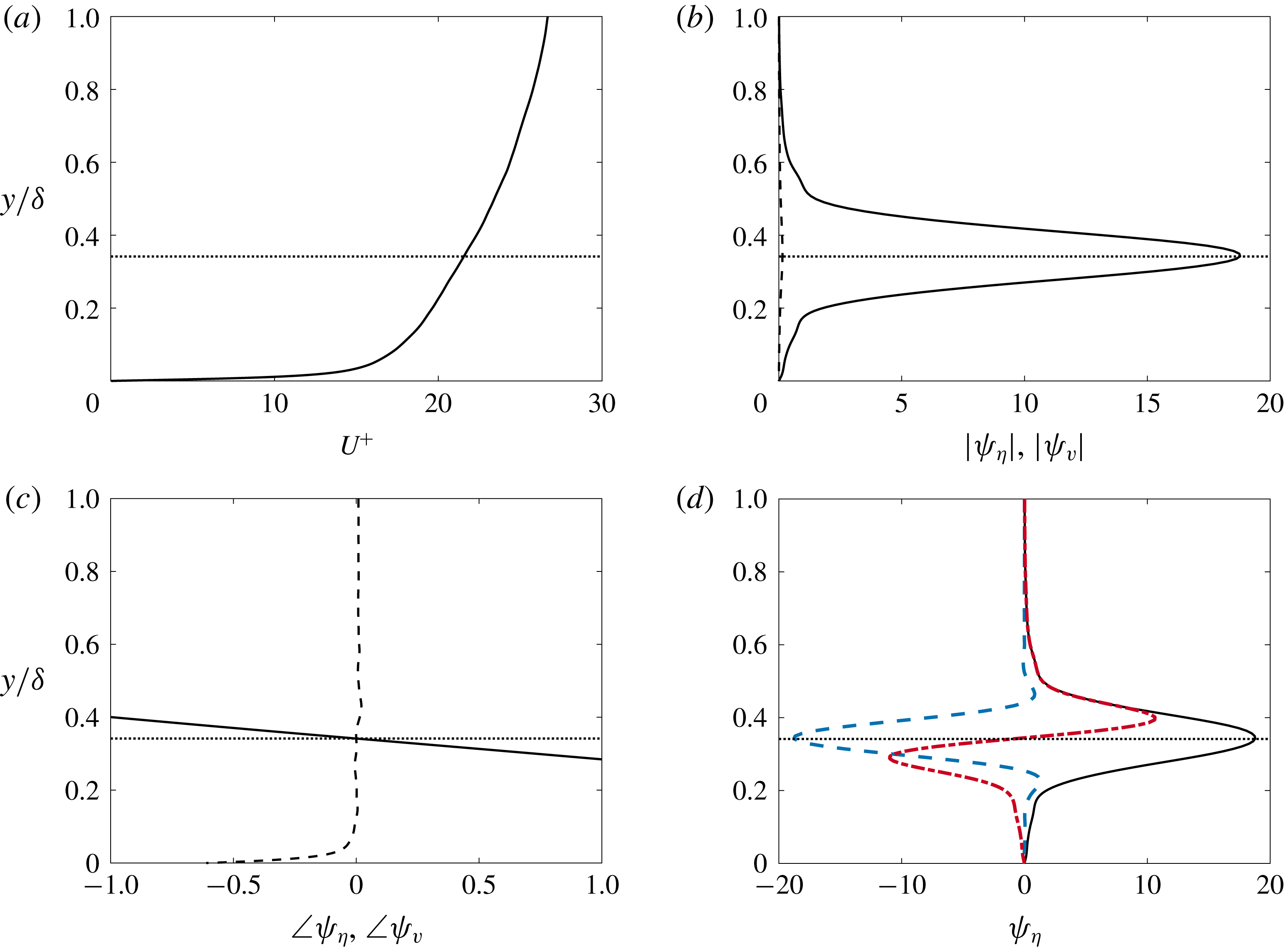
. Mean velocity profiles are obtained from the direct numerical simulation data of Wu et al. (Reference Wu, Moin, Wallace, Skarda, Lozano-Durán and Hickey2017), by averaging data (in both time and in the spanwise direction) at a single streamwise location. Figure 1 shows typical leading resolvent response mode shapes for this system, and in particular the ‘wavepacket’ nature of such modes. The wavenumbers
 $k_{x}=\unicode[STIX]{x03C0}/2$
, and
 $k_{z}=2\unicode[STIX]{x03C0}$
and wave speed (
 $c=0.8U_{\infty }$
) have been chosen to be consistent with the typical size of large-scale motions in zero-pressure-gradient boundary layers (e.g. Kovasznay, Kibens & Blackwelder (Reference Kovasznay, Kibens and Blackwelder1970), Cantwell (Reference Cantwell1981), Monty et al. (Reference Monty, Hutchins, Ng, Marusic and Chong2009), Saxton-Fox & McKeon (Reference Saxton-Fox and McKeon2017)). Here and throughout, the resolvent operator is discretised using a Chebyshev collocation method, utilising the toolbox of Weideman & Reddy (Reference Weideman and Reddy2000).
We observe that the mode is dominated by the wall-normal vorticity component, which is centred on and localised around the critical layer, and has an approximately linear variation in phase within this region. These observations, which are typical of modes that are ‘detached’ from the wall, suggests that this numerically computed mode resembles a wavepacket mode as described in § 2.3. Here and throughout, we consider a mode to be detached from the wall if its shape is not substantially affected by the wall’s presence. In § 4 we will seek to predict the shape of this mode without explicitly computing an SVD (or indeed, without explicitly forming a discretised resolvent operator). Making this procedure tractable, however, will require simplification of the governing equations, which are described in § 3.2.
(a) Mean velocity profile for a turbulent boundary layer at
 $Re_{\unicode[STIX]{x1D70F}}=900$
(solid line) and critical layer location (dotted) corresponding to a wave speed
 $c=0.8U_{\infty }$
. (b) Amplitude and (c) phase of wall-normal velocity (dashed) and vorticity (solid) for leading resolvent response modes with
 $k_{x}=\unicode[STIX]{x03C0}/2$
,
 $k_{z}=2\unicode[STIX]{x03C0}$
and
 $c=0.8U_{\infty }$
. (d) Shows the real (blue dashed) and imaginary (red dot-dashed) parts of the wall-normal vorticity component of this mode.

3.2 Simplifications to the Navier–Stokes operator for resolvent mode approximation
Following Rosenberg & McKeon (Reference Rosenberg and McKeon2019), rather than studying the full system we may start by separating the resolvent modes into those being forced by
 $f_{v}$
and
 $f_{\unicode[STIX]{x1D702}}$
separately. In particular, defining scalar resolvent operators
 $$\begin{eqnarray}\displaystyle & \displaystyle {\mathcal{H}}_{vv}=(-\text{i}\unicode[STIX]{x1D714}+\unicode[STIX]{x1D6E5}^{-1}{\mathcal{L}}_{os})^{-1}, & \displaystyle\end{eqnarray}$$
 $$\begin{eqnarray}\displaystyle & \displaystyle {\mathcal{H}}_{\unicode[STIX]{x1D702}\unicode[STIX]{x1D702}}=(-\text{i}\unicode[STIX]{x1D714}+{\mathcal{L}}_{sq})^{-1}, & \displaystyle\end{eqnarray}$$
the Orr–Sommerfeld and Squire modes may be computed by taking SVDs of the reduced resolvent operators given as
 $$\begin{eqnarray}\displaystyle & \displaystyle \left(\begin{array}{@{}c@{}}\hat{v}\\ \hat{\unicode[STIX]{x1D702}}_{os}\end{array}\right)=\underbrace{\left(\begin{array}{@{}cc@{}}{\mathcal{H}}_{vv} & 0\\ -\text{i}k_{z}{\mathcal{H}}_{\unicode[STIX]{x1D702}\unicode[STIX]{x1D702}}U_{y}{\mathcal{H}}_{vv} & 0\end{array}\right)}_{{\mathcal{H}}_{os,\boldsymbol{k}}}\left(\begin{array}{@{}c@{}}{\hat{g}}_{v}\\ 0\end{array}\right), & \displaystyle\end{eqnarray}$$
 $$\begin{eqnarray}\displaystyle & \displaystyle \left(\begin{array}{@{}c@{}}0\\ \hat{\unicode[STIX]{x1D702}}_{sq}\end{array}\right)=\underbrace{\left(\begin{array}{@{}cc@{}}0 & 0\\ 0 & {\mathcal{H}}_{\unicode[STIX]{x1D702}\unicode[STIX]{x1D702}}\end{array}\right)}_{{\mathcal{H}}_{sq,\boldsymbol{k}}}\left(\begin{array}{@{}c@{}}0\\ {\hat{g}}_{\unicode[STIX]{x1D702}}\end{array}\right). & \displaystyle\end{eqnarray}$$
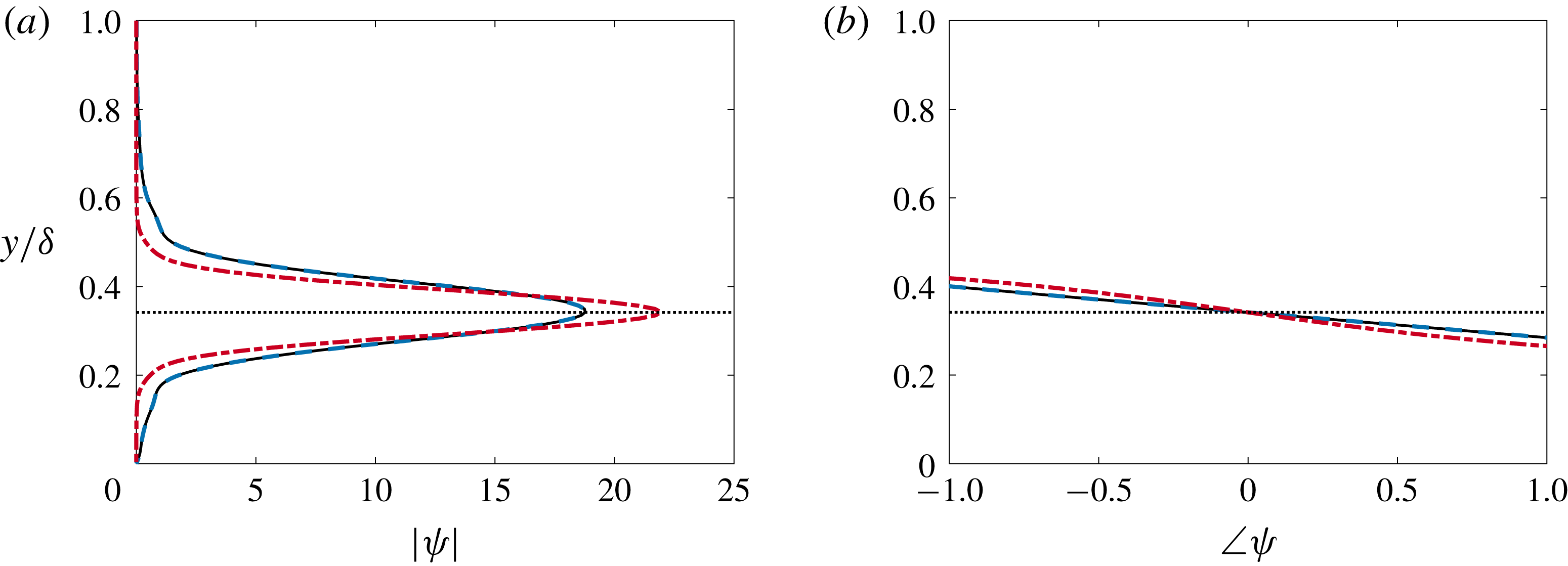
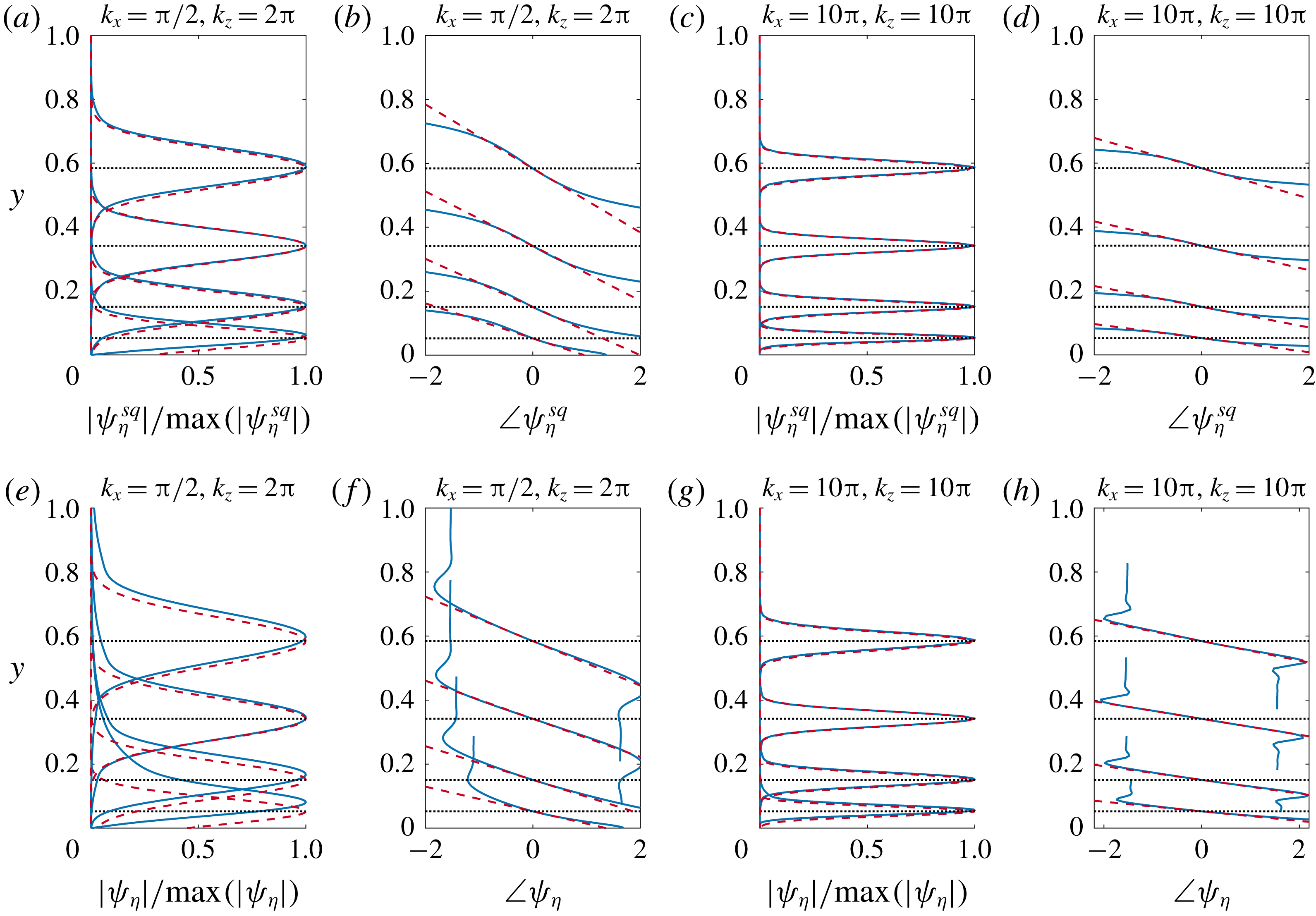
While the modes computed from different subsystems are no longer orthogonal, Rosenberg & McKeon (Reference Rosenberg and McKeon2019) demonstrated they can provide a basis that better captures dynamical features of the system. Our interest in this decomposition is primarily concerned with using this decomposition to simplify the required analysis. Figure 2 shows the
 $\unicode[STIX]{x1D702}$
-component of the response modes of the OS and SQ subsystems for the same parameters considered in figure 1. We observe in particular that the OS operator gives the same mode shape as the full system, with the SQ mode also sharing the same qualitative characteristics. This suggests that the ability to predict and understand the shape of the vorticity response of the full system can be reduced to studying only the OS subsystem.
In order to make the ensuing analysis more tractable, we will require additional simplifications. Note first that the components of the OS and SQ sub-operators may be written in scalar form as
 $$\begin{eqnarray}\displaystyle & \displaystyle \hat{v}={\mathcal{H}}_{vv}{\hat{g}}_{v}, & \displaystyle\end{eqnarray}$$
 $$\begin{eqnarray}\displaystyle & \displaystyle \hat{\unicode[STIX]{x1D702}}_{os}={\mathcal{H}}_{\unicode[STIX]{x1D702}v}{\hat{g}}_{v}, & \displaystyle\end{eqnarray}$$
 $$\begin{eqnarray}\displaystyle & \displaystyle \hat{\unicode[STIX]{x1D702}}_{sq}={\mathcal{H}}_{\unicode[STIX]{x1D702}\unicode[STIX]{x1D702}}{\hat{g}}_{\unicode[STIX]{x1D702}}, & \displaystyle\end{eqnarray}$$
where
 ${\mathcal{H}}_{\unicode[STIX]{x1D702}v}=-(\text{i}k_{z}{\mathcal{H}}_{\unicode[STIX]{x1D702}\unicode[STIX]{x1D702}}U_{y}{\mathcal{H}}_{vv})$
is the off-diagonal term in
 ${\mathcal{H}}_{os,\boldsymbol{k}}$
in (3.9).
(a) Amplitude and (b) phase of wall-normal vorticity response mode computed from full system (solid lines), SQ subsystem (red dot-dashed) and OS subsystem (blue dashed), with the same parameters as in figure 1.

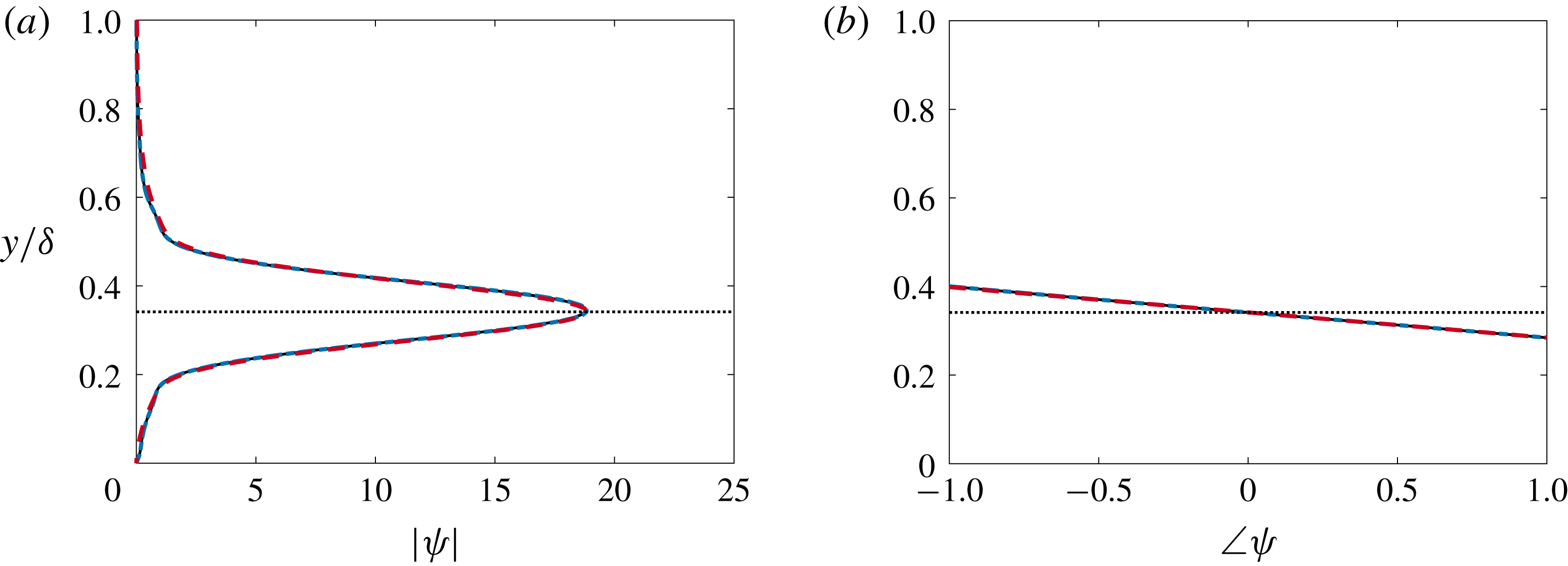
(a) Amplitude and (b) phase of wall-normal vorticity response mode computed from the OS subsystem (solid lines), the scalar off-diagonal term
 ${\mathcal{H}}_{\unicode[STIX]{x1D702}v}$
of the OS subsystem (blue dot-dashed) and its simplified scalar approximation computed using
 ${\mathcal{H}}_{\unicode[STIX]{x1D702}\unicode[STIX]{x1D702}}$
with a Laplacian inner product (red dashed), all with the same parameters as in figure 1.

When considering the SVD of these subsystems, it is important that we use the appropriate inner product on both the input and output spaces. Since the response is energetically dominated by wall-normal vorticity, it is reasonable that a close approximation to the
 $\unicode[STIX]{x1D702}$
response of the full system (which itself is approximated by the OS response) can be obtained just by considering the scalar operator in (3.12). Figure 3 shows that this assumption is indeed valid for the sample parameters considered in this section. As well as simplifying the analysis, reducing the full resolvent operator to a scalar operator brings us closer to being able to apply the wavepacket pseudomode theory discussed in § 2.3. An additional requirement for the direct application of this theory is that the operator under consideration be representable as a differential operator in the form of (2.16). The operator in (3.12) does not satisfy this property, as the OS component contains the inverse Laplacian.
Motivated by this, we now present an approximating simplification to (2.16), which we believe to be novel. This development will take advantage of the similarity between the OS and SQ operators, and will consider variations of the ‘standard’ inner products discussed in § 3.1. We start by taking a Taylor series expansion of the mean velocity profile about the critical layer location
 $y_{c}$
,
 $$\begin{eqnarray}\displaystyle U(y)=U(y_{c})+U_{y_{c}}(y-y_{c})+{\textstyle \frac{1}{2}}U_{y_{c}^{2}}(y-y_{c})^{2}+\cdots \,, & & \displaystyle\end{eqnarray}$$
where
 $U_{y_{c}}$
and
 $U_{y_{c}^{2}}$
are the first and second derivatives of
 $U(y)$
in the wall-normal direction at
 $y=y_{c}$
. If we are considering modes that are localised about the critical layer, it is reasonable to truncate this expansion. In particular, we reason that the amplification mechanism giving modes such as those observed in figures 1 and 2 is primarily due to the linear term in (3.14) (i.e. the local shear at the critical layer). Neglecting higher derivatives of the mean velocity, we have
 $$\begin{eqnarray}\displaystyle {\mathcal{H}}_{vv}=\unicode[STIX]{x1D6E5}^{-1}{\mathcal{H}}_{\unicode[STIX]{x1D702}\unicode[STIX]{x1D702}}\unicode[STIX]{x1D6E5}. & & \displaystyle\end{eqnarray}$$
This means that the operator that we are attempting to simplify is
 $$\begin{eqnarray}\displaystyle {\mathcal{H}}_{\unicode[STIX]{x1D702}v}^{Lin} & = & \displaystyle -(\text{i}k_{z}U_{y_{c}}){\mathcal{H}}_{\unicode[STIX]{x1D702}\unicode[STIX]{x1D702}}{\mathcal{H}}_{vv}\nonumber\\ \displaystyle & = & \displaystyle -(\text{i}k_{z}U_{y_{c}}){\mathcal{H}}_{\unicode[STIX]{x1D702}\unicode[STIX]{x1D702}}\unicode[STIX]{x1D6E5}^{-1}{\mathcal{H}}_{\unicode[STIX]{x1D702}\unicode[STIX]{x1D702}}\unicode[STIX]{x1D6E5},\end{eqnarray}$$
where the
 $Lin$
superscript denotes that the mean velocity profile has been linearised about
 $y_{c}$
.
Figure 3 shows that the leading response mode of
 ${\mathcal{H}}_{\unicode[STIX]{x1D702}v}$
matches the
 $\unicode[STIX]{x1D702}$
-component of that for the full Navier–Stokes system, while in figure 2 we observe that the leading response mode of
 ${\mathcal{H}}_{\unicode[STIX]{x1D702}\unicode[STIX]{x1D702}}$
does not quantitatively match that for the full system, and thus does not match the mode from
 ${\mathcal{H}}_{\unicode[STIX]{x1D702}v}$
. This difference arises from the fact that amplification of forcing through the operator
 ${\mathcal{H}}_{\unicode[STIX]{x1D702}v}$
will depend on the properties of both
 ${\mathcal{H}}_{\unicode[STIX]{x1D702}\unicode[STIX]{x1D702}}$
and
 ${\mathcal{H}}_{vv}$
, and in particular because the leading forcing mode of
 ${\mathcal{H}}_{\unicode[STIX]{x1D702}\unicode[STIX]{x1D702}}$
does not coincide with the most amplified response mode of
 ${\mathcal{H}}_{vv}$
. Physically, leading resolvent modes of the operator
 ${\mathcal{H}}_{\unicode[STIX]{x1D702}\unicode[STIX]{x1D702}}$
represent amplification due to the Orr mechanism (with forcing and response both in the
 $\unicode[STIX]{x1D702}$
-direction), while those of
 ${\mathcal{H}}_{\unicode[STIX]{x1D702}v}$
correspond to the lift-up mechanism, where forcing in the
 $v$
-component is ‘lifted’ to give a response in
 $\unicode[STIX]{x1D702}$
.
Given that the leading resolvent modes are dependent on the choice of inner product, it is reasonable to ask if a different choice of inner product could be used in the SVD of
 ${\mathcal{H}}_{\unicode[STIX]{x1D702}\unicode[STIX]{x1D702}}$
, such that the leading forcing mode approximately coincides with the leading response of
 ${\mathcal{H}}_{vv}$
. Physically, what we are seeking to do is to find an inner product weighting that will allow us to study the properties of the lift-up mechanism using the (simpler) operator that is typically associated with the Orr mechanism.
Let
 ${\mathcal{H}}_{\unicode[STIX]{x1D702}\unicode[STIX]{x1D702}}^{\ast }$
denote the adjoint of
 ${\mathcal{H}}_{\unicode[STIX]{x1D702}\unicode[STIX]{x1D702}}$
with respect to the standard scalar inner product, equation (3.5). If we instead consider the ‘Laplacian’ inner product, we obtain
 $$\begin{eqnarray}\displaystyle {\mathcal{H}}_{\unicode[STIX]{x1D702}\unicode[STIX]{x1D702}}^{\ast ,\unicode[STIX]{x1D6E5}}=\unicode[STIX]{x1D6E5}^{-1}{\mathcal{H}}_{\unicode[STIX]{x1D702}\unicode[STIX]{x1D702}}^{\ast }\unicode[STIX]{x1D6E5}. & & \displaystyle\end{eqnarray}$$
This has the same form as (3.15), except with the (standard) adjoint of
 ${\mathcal{H}}_{\unicode[STIX]{x1D702}\unicode[STIX]{x1D702}}$
, which amounts to taking the complex conjugate of the critical layer term. Note also that
 ${\mathcal{H}}_{\unicode[STIX]{x1D702}\unicode[STIX]{x1D702}}$
with the regular inner product has leading forcing and response modes (i.e. right and left singular vectors) that differ only in the direction of the phase change. We also then have
 $$\begin{eqnarray}\displaystyle ({\mathcal{H}}_{\unicode[STIX]{x1D702}\unicode[STIX]{x1D702}}^{\ast })^{\ast ,\unicode[STIX]{x1D6E5}}=\unicode[STIX]{x1D6E5}^{-1}{\mathcal{H}}_{\unicode[STIX]{x1D702}\unicode[STIX]{x1D702}}\unicode[STIX]{x1D6E5}, & & \displaystyle\end{eqnarray}$$
which is identical to (3.15), meaning in particular that both share the same resolvent forcing and response modes. If we are to weight this operator explicitly to compute an SVD in the Laplacian scalar norm, we obtain
 $$\begin{eqnarray}\displaystyle {\mathcal{H}}_{vv}^{W,\unicode[STIX]{x1D6E5}}=[({\mathcal{H}}_{\unicode[STIX]{x1D702}\unicode[STIX]{x1D702}}^{\ast })^{\ast ,\unicode[STIX]{x1D6E5}}]^{W,\unicode[STIX]{x1D6E5}}=\unicode[STIX]{x1D6E5}^{-1/2}{\mathcal{H}}_{\unicode[STIX]{x1D702}\unicode[STIX]{x1D702}}\unicode[STIX]{x1D6E5}^{1/2}. & & \displaystyle\end{eqnarray}$$
Therefore, computing this SVD should give a leading forcing mode for
 ${\mathcal{H}}_{\unicode[STIX]{x1D702}\unicode[STIX]{x1D702}}$
that coincides with the leading response mode of
 ${\mathcal{H}}_{vv}$
, thus minimising the ‘projection loss’ of the total amplification. In effect, we are modifying the inner product used for
 ${\mathcal{H}}_{\unicode[STIX]{x1D702}\unicode[STIX]{x1D702}}$
such that its leading forcing mode aligns with the leading response mode of
 ${\mathcal{H}}_{vv}$
. This analysis therefore relies on the assumption that the total amplification is dominated by the lift-up, rather than the Orr, mechanism. With this assumption, this trick allows us to compute optimal response mode shapes by only considering the Squire operator, which is a differential operator of the general form given in (2.15), rather than the full OS operator, which is not. It will be shown later that this assumption holds except for large
 $k_{\bot }^{2}$
, in which case the Laplacian approaches a constant, and so
 ${\mathcal{H}}_{\unicode[STIX]{x1D702}\unicode[STIX]{x1D702}}$
and
 ${\mathcal{H}}_{vv}$
converge to the same operator. Note, however, that this simplification will not in general be able to directly predict the singular values (resolvent gains) corresponding to the predicted mode shapes, except for in this large
 $k_{\bot }^{2}$
regime. Figure 3 shows that this modification to the inner product allows us to closely match the wall-normal vorticity component of the response mode of the full Navier–Stokes system, for the sample parameters chosen. We will further explore the validity of this approximation in § 5.
4 Methods for predicting the shape of resolvent modes
This section will present a method that allows for the prediction of resolvent response mode shapes. The main idea will be to first assume the existence of a mode that is localised in both wall-normal location, and wall-normal spatial frequency (i.e. a linear variation in phase in the wall-normal direction). We then find the parameters corresponding to maximum amplification of the resolvent operator, or equivalently, minimisation of the action of its inverse, on a given function. In this section we will focus on a model operator, which is closely related to the Squire operator. In § 4.1 we relate resolvent mode shapes for this operator to asymptotic expansions of Airy functions, before we present in § 4.2 a method to analytically determine the relevant mode shape parameters for this operator under the assumption of the existence of wavepacket pseudomodes. This latter approach will later be extended to consider the shape of modes for the full incompressible Navier–Stokes system in § 5.
4.1 Relationship between wavepacket resolvent modes and Airy functions
Before applying wavepacket pseudomode theory more generally, in this section we focus on a model (Airy) operator that is equivalent to the Squire operator with a linearised mean velocity profile. This analysis will show how numerically computed resolvent response modes relate to exact analytical solutions to simplified governing equations. Linearising the mean velocity profile about the critical layer, the Squire equation reduces to
 $$\begin{eqnarray}\displaystyle (-\text{i}\unicode[STIX]{x1D714}+{\mathcal{L}}_{sq}^{Lin})=\text{i}k_{x}U_{y_{c}}(y-y_{c})-Re^{-1}\unicode[STIX]{x1D6E5}. & & \displaystyle\end{eqnarray}$$
For clarity, we let
 $R=k_{x}U_{y_{c}}Re$
, and consider the closely related operator
 $$\begin{eqnarray}\displaystyle {\mathcal{T}}=(\text{i}k_{x}U_{y_{c}})^{-1}(-\text{i}\unicode[STIX]{x1D714}+{\mathcal{L}}_{sq}^{Lin}) & = & \displaystyle -(\text{i}R)^{-1}\frac{\text{d}^{2}}{\text{d}y^{2}}+(y-y_{c}+(\text{i}R)^{-1}k_{\bot }^{2})\nonumber\\ \displaystyle & = & \displaystyle -(\text{i}R)^{-1}\frac{\text{d}^{2}}{\text{d}y^{2}}+(y-y_{c}-\unicode[STIX]{x1D714}_{c}i)\nonumber\\ \displaystyle & = & \displaystyle -(\text{i}R)^{-1}\frac{\text{d}^{2}}{\text{d}y^{2}}+(y-\unicode[STIX]{x1D706}),\end{eqnarray}$$
where
 $\unicode[STIX]{x1D706}=y_{c}+\unicode[STIX]{x1D714}_{c}\text{i}$
, and
 $\unicode[STIX]{x1D714}_{c}=R^{-1}k_{\bot }^{2}$
, and we are assuming that
 $k_{x}\neq 0$
. Note that we are generally interested in performing resolvent analysis along the axis of neutral stability (i.e. for real-valued frequencies with no growth or decay), but here we are incorporating the viscous dissipation term
 $\unicode[STIX]{x1D714}_{c}$
into
 $\unicode[STIX]{x1D706}$
, so in general
 $\unicode[STIX]{x1D706}$
is complex for this analysis.
 ${\mathcal{T}}$
is a complex Airy-type operator, and is identical to the operator considered, for example, in Reddy, Schmid & Henningson (Reference Reddy, Schmid and Henningson1993) as a model for studying the pseudospectra of the Orr–Sommerfeld operator. The equation
 ${\mathcal{T}}u=0$
has a general solution that can be expressed by two independent Airy functions, such as
 $$\begin{eqnarray}\displaystyle u(y)=c_{1}A\text{i}[z]+c_{2}A\text{i}[\text{e}^{2\unicode[STIX]{x03C0}\text{i}/3}z], & & \displaystyle\end{eqnarray}$$
with
 $$\begin{eqnarray}\displaystyle z=(\text{i}R)^{1/3}(y-\unicode[STIX]{x1D706}). & & \displaystyle\end{eqnarray}$$
Note that distinct solutions are obtained through the choice of contour in the complex plane when applying standard Laplace transform methods.
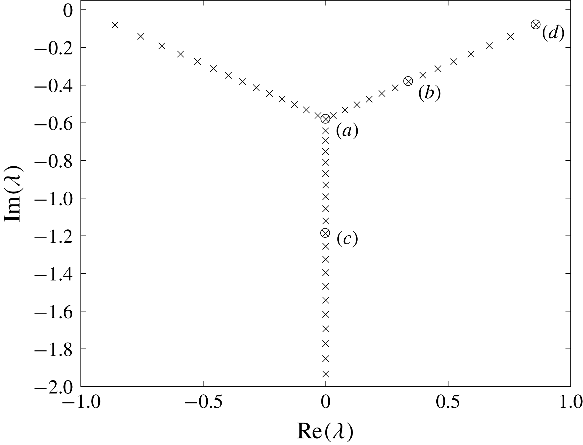
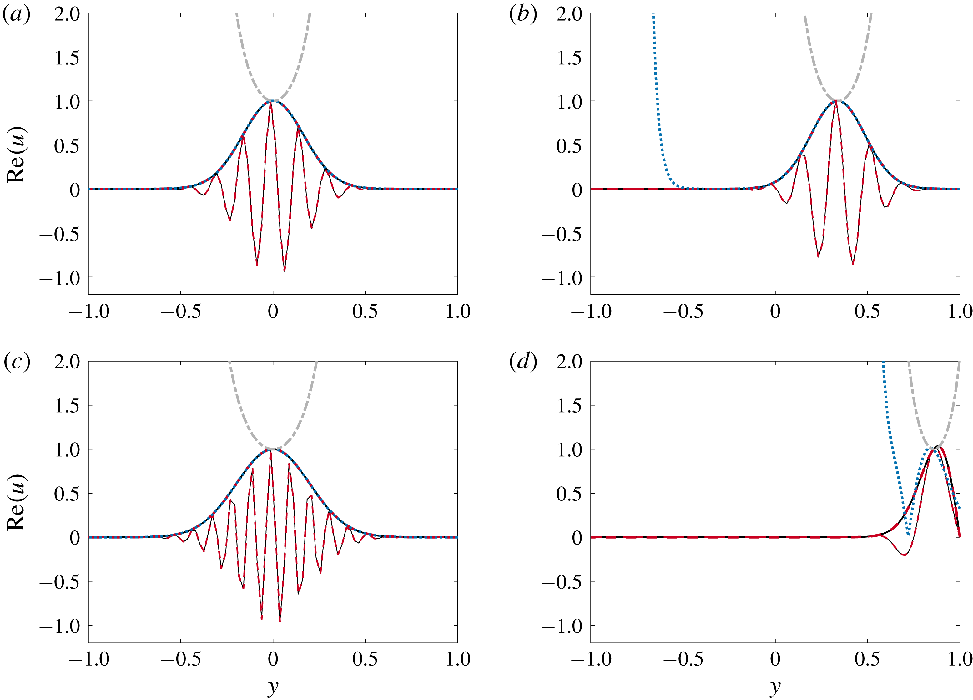
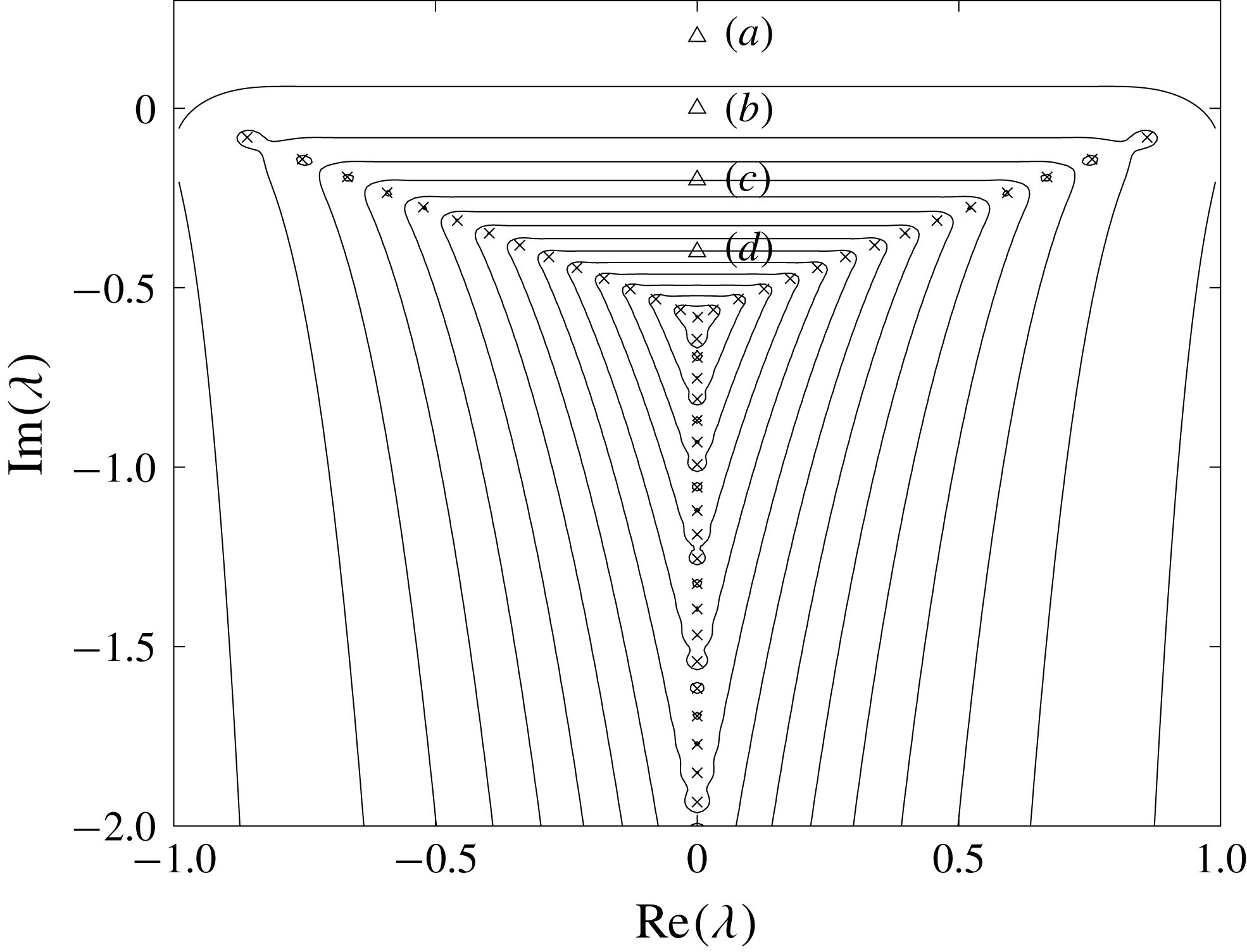
Shown in figure 4 are eigenvalues of
 ${\mathcal{T}}$
with Dirichlet boundary conditions on a finite domain
 $y\in [-1,1]$
, with
 $R=3000$
. In figure 5, these numerical eigenmodes are compared to the Airy functions
 $\text{Ai}[z]$
,
 $\text{Ai}[\text{e}^{2\unicode[STIX]{x03C0}\text{i}/3}z]$
and
 $\text{Ai}[\text{e}^{-2\unicode[STIX]{x03C0}\text{i}/3}z]$
. We observe that the
 $\text{Ai}[\text{e}^{2\unicode[STIX]{x03C0}\text{i}/3}z]$
solution (when appropriately scaled) closely matches all of the numerically computed eigenmodes on this finite domain. Note that these eigenvalues are symmetric about
 $\text{Re}(\unicode[STIX]{x1D706})=0$
, and if we had chosen eigenvalues on the left branch (i.e. with negative real component), then the
 $\text{Ai}[z]$
solution would have instead been accurate for all cases.
Spectrum of
 ${\mathcal{T}}$
with Dirichlet boundary conditions on the domain
 $y\in [-1,1]$
, with
 $R=3000$
. Circled and labelled eigenvalues correspond to eigenmodes plotted in figure 5.

Comparison between numerically computed eigenmodes (solid lines) of
 ${\mathcal{T}}$
with
 $R=3000$
, and scaled analytic solutions of the Airy equation
 $\text{Ai}[\text{e}^{2\unicode[STIX]{x03C0}\text{i}/3}z]$
(red dashed),
 $\text{Ai}[z]$
(blue dotted) and
 $\text{Ai}[\text{e}^{-2\unicode[STIX]{x03C0}\text{i}/3}z]$
(grey dot-dashed). Plotted eigenmodes are those identified by labels (a–d) in figure 4. Mode amplitudes are plotted for all cases, with real components also plotted with thinner lines for the numerical mode and the
 $\text{Ai}[\text{e}^{2\unicode[STIX]{x03C0}i/3}z]$
Airy function.

On an infinite domain (and when acting on square-integrable functions)
 ${\mathcal{T}}$
has an empty spectrum, and
 $\unicode[STIX]{x1D716}$
-pseudospectra that are independent of location on the real axis (that is, the boundaries of the pseudospectrum for various
 $\unicode[STIX]{x1D716}$
are horizontal lines). This empty spectrum directly relates to the fact that all Airy function solutions to the eigenvalue problem
 ${\mathcal{T}}u(y)=\unicode[STIX]{x1D706}u(y)$
diverge at as
 $y\rightarrow \infty$
or
 $y\rightarrow -\infty$
(or both).
As discussed in Reddy et al. (Reference Reddy, Schmid and Henningson1993), a solution to
 ${\mathcal{T}}u=0$
which is within
 $\unicode[STIX]{x1D716}$
of a function that satisfies the appropriate boundary conditions will be an
 $\unicode[STIX]{x1D716}$
-pseudoeigenfunction. We consider the pseudospectra of
 ${\mathcal{T}}$
, again for the finite domain
 $y\in [-1,1]$
. As discussed in § 2.2, this amounts to computing the leading singular values and vectors of the resolvent of
 ${\mathcal{T}}$
for each
 $\unicode[STIX]{x1D706}\in \mathbb{C}$
of interest. In particular, we may seek analytic approximations of these resolvent (optimal pseudospectral) modes using the same method as for eigenfunctions. In other words, for a given
 $\unicode[STIX]{x1D706}\in \mathbb{C}$
, we are interested in finding a function which is as close as possible to an eigenmode of
 ${\mathcal{T}}$
. Noting that the Airy functions are continuous, the fact that there are regions of
 $\mathbb{C}$
for which they are very close to satisfying the boundary conditions of the finite domain suggest that these regions correspond to very large values of resolvent norm
 $\unicode[STIX]{x1D70E}_{1}$
.
The
 $\unicode[STIX]{x1D716}$
-pseudospectra overlaid on the spectrum of
 ${\mathcal{T}}$
, with parameters equal to those for figures 4 and 5. Pseudospectra contour levels are
 $\unicode[STIX]{x1D716}\in \{10^{-15},10^{-14},\ldots ,10^{-1}\}$
. Triangles represent locations corresponding to resolvent modes plotted in figure 7.

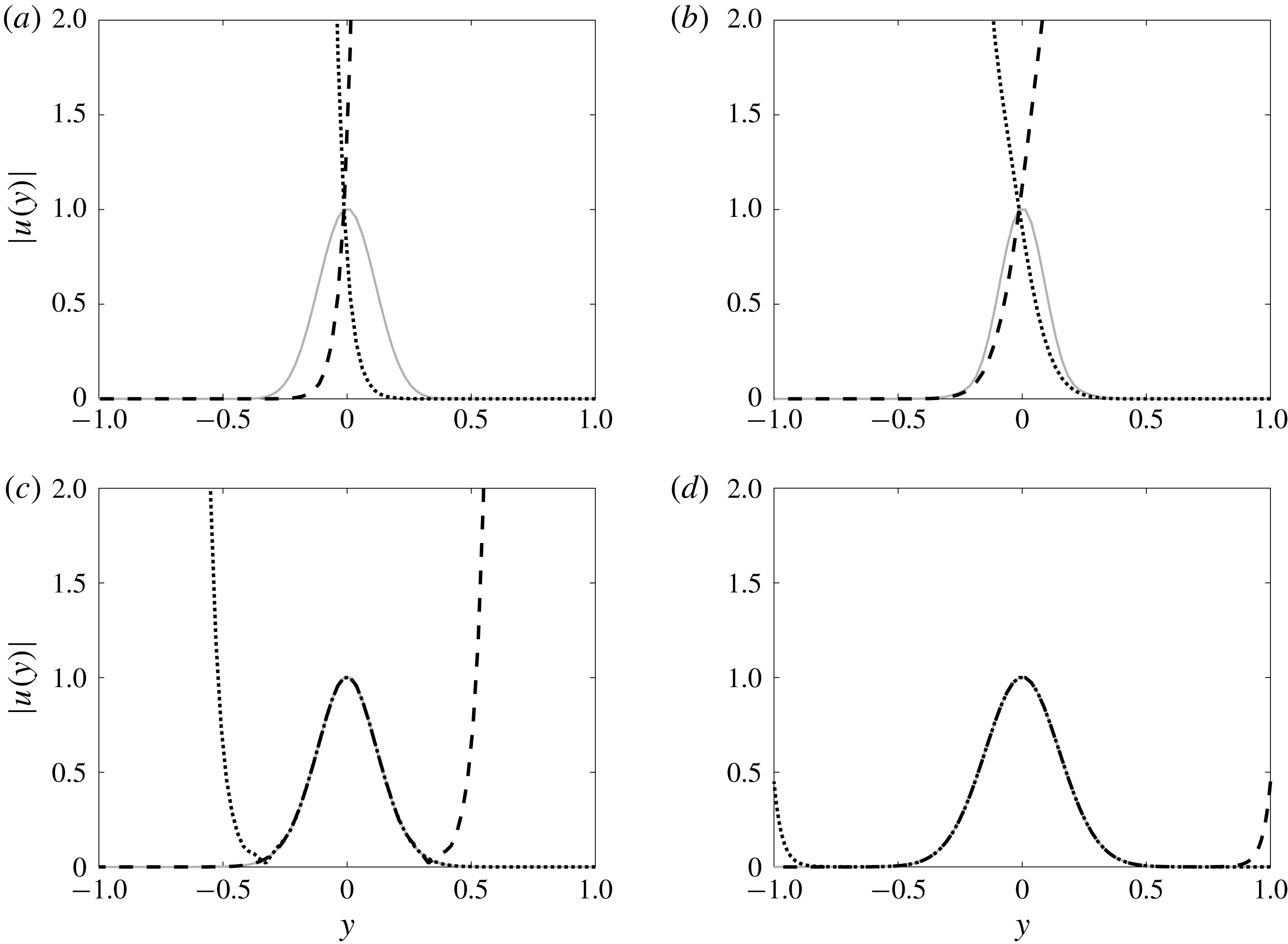
Amplitudes of numerically computed resolvent modes (grey solid lines) for locations in
 $\mathbb{C}$
as indicated by labels (a–d) in figure 6, compared with amplitudes of Airy functions
 $\text{Ai}[z]$
(dotted), and
 $\text{Ai}[\text{e}^{2\unicode[STIX]{x03C0}\text{i}/3}z]$
(dashed).

Figure 6 shows
 $\unicode[STIX]{x1D716}$
-pseudospectra for
 ${\mathcal{T}}$
. In the central region away from the boundaries, the pseudospectral properties of
 ${\mathcal{T}}$
resemble that of the operator on an infinite domain, where resolvent modes, which are ‘detached’ from the boundary, are invariant to horizontal translation within this region. Moreover, resolvent modes within this region will resemble translated versions of eigenmodes along the inclined branches of eigenvalues at the same vertical position. Optimal pseudoeigenmodes (i.e. resolvent modes), and Airy function approximations thereof, are shown in figure 7. We observe that, as
 $\unicode[STIX]{x1D716}$
increases and we approach the real axis, the analytical Airy functions become less accurate, owing to their divergent growth in amplitude occurring closer and closer to the critical layer, eventually saturating the component resembling the numerically computed response mode. Note that this behaviour means that it is impossible to find linear combinations of Airy functions (such as that given in (4.3)) that accurately approximate these modes everywhere in the domain. Only the amplitude of the numerical and analytic functions are shown in figure 7, although we find that the phase of the numerical and analytic functions closely match in the region where the amplitudes agree.
As discussed in Reddy et al. (Reference Reddy, Schmid and Henningson1993), these Airy functions can be used to compute constructive lower bounds to the pseudospectrum of
 ${\mathcal{T}}$
, although these bounds are inaccurate whenever the Airy functions diverge far away from
 $y=\text{Re}(\unicode[STIX]{x1D706})$
. The fact that
 $\unicode[STIX]{x1D714}_{c}=R^{-1}k_{\bot }^{2}$
means that the most physically relevant region of the complex plane is in the upper half-plane, which means that the Airy functions themselves are not close approximations of physically relevant resolvent modes.
Away from the origin, one may approximate Airy functions by simpler expressions that do not involve integrals. The derivation of such asymptotic approximations involves finding a location in the complex that has a dominant contribution to the contour integral. We may derive the approximation (e.g. Vallée & Soares Reference Vallée and Soares2010; Olver Reference Olver2014)
 $$\begin{eqnarray}\displaystyle \text{Ai}(z)\approx {\textstyle \frac{1}{2}}\sqrt{\unicode[STIX]{x03C0}}z^{-1/4}\exp \left(-{\textstyle \frac{2}{3}}z^{3/2}\right)\sim \exp \left(-{\textstyle \frac{2}{3}}z^{3/2}\right), & & \displaystyle\end{eqnarray}$$
which is accurate for large
 $|z|$
. Here
 $z=\unicode[STIX]{x1D6FE}(y-\unicode[STIX]{x1D706})$
, where (with reference to (4.4)) we have
 $\unicode[STIX]{x1D6FE}=(\text{i}R)^{1/3}$
,
 $\unicode[STIX]{x1D706}=\text{i}k_{\bot }^{2}/R=\text{i}\unicode[STIX]{x1D714}_{c}$
, and we assume for now that
 $y_{c}=0$
. Expanding the exponential term gives
 $$\begin{eqnarray}\displaystyle \exp \left(-\frac{2}{3}z^{3/2}\right)=\exp \left[-\frac{2}{3}(-\unicode[STIX]{x1D706}\unicode[STIX]{x1D6FE})^{3/2}\left(1-\frac{3}{2}\frac{y}{\unicode[STIX]{x1D706}}+\frac{3}{8}\left(\frac{y}{\unicode[STIX]{x1D706}}\right)^{2}-\cdots \,\right)\right], & & \displaystyle\end{eqnarray}$$
and thus
 $$\begin{eqnarray}\displaystyle \text{Ai}(z)\sim C\exp \left[(-\unicode[STIX]{x1D706}\unicode[STIX]{x1D6FE})^{3/2}\frac{y}{\unicode[STIX]{x1D706}}-\frac{1}{4}(-\unicode[STIX]{x1D706}\unicode[STIX]{x1D6FE})^{3/2}\left(\frac{y}{\unicode[STIX]{x1D706}}\right)^{2}-\cdots \,\right], & & \displaystyle\end{eqnarray}$$
where we must take care when dealing with multi-valued roots. In particular, for a bounded approximation, we require that
 $$\begin{eqnarray}\displaystyle \text{Re}[(-\unicode[STIX]{x1D706}\unicode[STIX]{x1D6FE})^{3/2}\unicode[STIX]{x1D706}^{-1}]=0. & & \displaystyle\end{eqnarray}$$
If
 $\unicode[STIX]{x1D706}=|\unicode[STIX]{x1D706}|\text{e}^{\text{i}\unicode[STIX]{x1D703}_{\unicode[STIX]{x1D706}}}$
, then we find that this condition is only satisfied when
 $\unicode[STIX]{x1D703}_{\unicode[STIX]{x1D706}}=3\unicode[STIX]{x03C0}/2$
. Note that this corresponds to the lower half-plane region where Airy functions can give close approximations to the numerically computed solutions. Assuming
 $y_{c}=0$
, so that
 $\unicode[STIX]{x1D706}=\unicode[STIX]{x1D714}_{c}\text{i}$
, for
 $\unicode[STIX]{x1D714}_{c}<0$
we obtain an approximation of the form
 $$\begin{eqnarray}\displaystyle \unicode[STIX]{x1D713}(y)\sim \exp \left[-\text{i}\sqrt{|\unicode[STIX]{x1D714}_{c}|R}y-\frac{1}{4}\sqrt{\frac{R}{|\unicode[STIX]{x1D714}_{c}|}}y^{2}\right]. & & \displaystyle\end{eqnarray}$$
4.2 Predicting wavepacket modes for a model operator
Section 4.1 demonstrated that, in certain regimes, resolvent modes may be approximated by a function of the general form
 $$\begin{eqnarray}\displaystyle \unicode[STIX]{x1D713}(y)=c\exp (\text{i}ay-by^{2}), & & \displaystyle\end{eqnarray}$$
where
 $a\in \mathbb{R}$
and
 $b>0$
are functions of
 $\unicode[STIX]{x1D714}_{c}$
and
 $R$
, and
 $$\begin{eqnarray}\displaystyle c=\left(\frac{2b}{\unicode[STIX]{x03C0}}\right)^{1/4}, & & \displaystyle\end{eqnarray}$$
is a constant that gives
 $\unicode[STIX]{x1D713}$
unit norm with respect to the regular scalar inner product.
This section will present an alternative analysis with this template function as a starting point. Applying wavepacket pseudomode theory as described in § 2.3, one may show that
 ${\mathcal{T}}$
satisfies the twist condition (2.18) within the half-strip
 $$\begin{eqnarray}\displaystyle \{\unicode[STIX]{x1D706}:-1<\text{Re}(\unicode[STIX]{x1D706})<1,\text{Im}(\unicode[STIX]{x1D706})<0\}. & & \displaystyle\end{eqnarray}$$
The
 $\text{Im}(\unicode[STIX]{x1D706})<0$
condition is consistent with the predicted condition for a spatially localised mode from the truncated asymptotic expansion of an Airy function in (4.9). Note that the region described in (4.12) is outside the region that is most physically relevant for resolvent analysis of the Squire operator, where a positive
 $k_{\bot }^{2}$
and
 $R$
give a positive imaginary component of
 $\unicode[STIX]{x1D714}_{c}$
. Despite this, figure 7(a) shows that even outside this region, the numerically computed pseudomode still maintains the same spatially localised structure. To predict the shape of resolvent modes outside this region, we will seek to directly optimise the shape parameters in the template function, equation (4.10). In particular, we wish to find the values of
 $a$
and
 $b$
for which
 $\Vert {\mathcal{T}}\unicode[STIX]{x1D713}\Vert$
is minimised, following the characterisation of the SVD in (2.10) and (2.11). That is, we seek the minimum of the cost function
 $$\begin{eqnarray}\displaystyle J_{{\mathcal{T}}}(a,b;R,\unicode[STIX]{x1D714}_{c})=\Vert {\mathcal{T}}\unicode[STIX]{x1D713}\Vert ^{2}=\int _{y=-\infty }^{\infty }({\mathcal{T}}\unicode[STIX]{x1D713})^{\ast }({\mathcal{T}}\unicode[STIX]{x1D713})\,\text{d}y, & & \displaystyle\end{eqnarray}$$
where we are assuming that our mode is ‘detached’ and localised, so we can integrate over an infinite domain, and are assuming a standard inner product for this model operator (note that including a constant multiplicative factor of
 $k_{\bot }^{-2}$
as in (3.5) does not affect mode shapes or singular values). For simplicity, we again take
 $y_{c}=0$
. Note that the leading resolvent singular value is related to this cost function by
 $$\begin{eqnarray}\displaystyle \unicode[STIX]{x1D70E}_{1}(R,\unicode[STIX]{x1D714}_{c})=[\min _{a,b}J_{{\mathcal{T}}}(a,b;R,\unicode[STIX]{x1D714}_{c})]^{-1/2}. & & \displaystyle\end{eqnarray}$$
Noting that we have
 $$\begin{eqnarray}\displaystyle & \displaystyle {\mathcal{T}}^{\ast }=(\text{i}R)^{-1}\frac{\text{d}^{2}}{\text{d}y^{2}}+(y+\text{i}\unicode[STIX]{x1D714}_{c}), & \displaystyle\end{eqnarray}$$
 $$\begin{eqnarray}\displaystyle & \displaystyle \unicode[STIX]{x1D713}^{\ast }(y)=c\exp [-\text{i}ay-by^{2}], & \displaystyle\end{eqnarray}$$
it can be shown that
 $$\begin{eqnarray}\displaystyle & \displaystyle {\mathcal{T}}\unicode[STIX]{x1D713}(y)=-\frac{1}{\text{i}R}[4b^{2}y^{2}-\text{i}(4ab+R)y-a^{2}-2b-R\unicode[STIX]{x1D714}_{c}]\unicode[STIX]{x1D713}(y), & \displaystyle\end{eqnarray}$$
 $$\begin{eqnarray}\displaystyle & \displaystyle ({\mathcal{T}}\unicode[STIX]{x1D713}(y))^{\ast }=\frac{1}{\text{i}R}[4b^{2}y^{2}+\text{i}(4ab+R)y-a^{2}-2b-R\unicode[STIX]{x1D714}_{c}]\unicode[STIX]{x1D713}^{\ast }(y). & \displaystyle\end{eqnarray}$$
From this, we may compute
 $$\begin{eqnarray}\displaystyle J_{{\mathcal{T}}}(a,b;R,\unicode[STIX]{x1D714}_{c})=\frac{1}{4b}+\frac{3}{R^{2}}b^{2}+\frac{2(3a^{2}+R\unicode[STIX]{x1D714}_{c})}{R^{2}}b+\frac{a^{4}+2aR+2\unicode[STIX]{x1D714}_{c}a^{2}R+\unicode[STIX]{x1D714}_{c}^{2}R^{2}}{R^{2}}.\quad & & \displaystyle\end{eqnarray}$$
We may analytically determine the locations of these minima as follows. This cost function is minimised when
 $$\begin{eqnarray}\displaystyle & \displaystyle \frac{\unicode[STIX]{x2202}J_{{\mathcal{T}}}}{\unicode[STIX]{x2202}a}=\frac{2}{R^{2}}(6ab+2a^{3}+2R\unicode[STIX]{x1D714}_{c}a+R)=0, & \displaystyle\end{eqnarray}$$
 $$\begin{eqnarray}\displaystyle & \displaystyle \frac{\unicode[STIX]{x2202}J_{{\mathcal{T}}}}{\unicode[STIX]{x2202}b}=-\frac{1}{4b^{2}}+\frac{2}{R^{2}}(3b+3a^{2}+R\unicode[STIX]{x1D714}_{c})=0. & \displaystyle\end{eqnarray}$$
Equations (4.20) and (4.21) may be solved to give the parameters
 $\{a,b\}$
minimising
 $J_{{\mathcal{T}}}$
, with care taken to select the correct minimising solution. It is also possible to obtain a parametrised family of solutions as follows. Assuming that
 $R$
is fixed, suppose that we seek the optimal values
 $(a(\unicode[STIX]{x1D714}_{c}),b(\unicode[STIX]{x1D714}_{c}))$
for a range of values of
 $\unicode[STIX]{x1D714}_{c}$
. By implicitly differentiating (4.20) and (4.21) with respect to
 $\unicode[STIX]{x1D714}_{c}$
, the following ordinary differential equations governing the evolution of the optimal mode shape parameters may be found:
 $$\begin{eqnarray}\displaystyle & \displaystyle \frac{\unicode[STIX]{x2202}a}{\unicode[STIX]{x2202}\unicode[STIX]{x1D714}_{c}}=\frac{-R^{3}a}{\unicode[STIX]{x1D714}_{c}R^{3}+3(a^{2}+b)R^{2}+12\unicode[STIX]{x1D714}_{c}b^{3}R+36b^{3}(b-a^{2})}, & \displaystyle\end{eqnarray}$$
 $$\begin{eqnarray}\displaystyle & \displaystyle \frac{\unicode[STIX]{x2202}b}{\unicode[STIX]{x2202}\unicode[STIX]{x1D714}_{c}}=\frac{-4b^{3}R(\unicode[STIX]{x1D714}_{c}R-3a^{2}+3b)}{\unicode[STIX]{x1D714}_{c}R^{3}+3(a^{2}+b)R^{2}+12\unicode[STIX]{x1D714}_{c}b^{3}R+36b^{3}(b-a^{2})}. & \displaystyle\end{eqnarray}$$
Note that this approach assumes that the global minimiser of
 $J_{{\mathcal{T}}}$
stays on the same branch, and is smoothly continuous with
 $\unicode[STIX]{x1D714}_{c}$
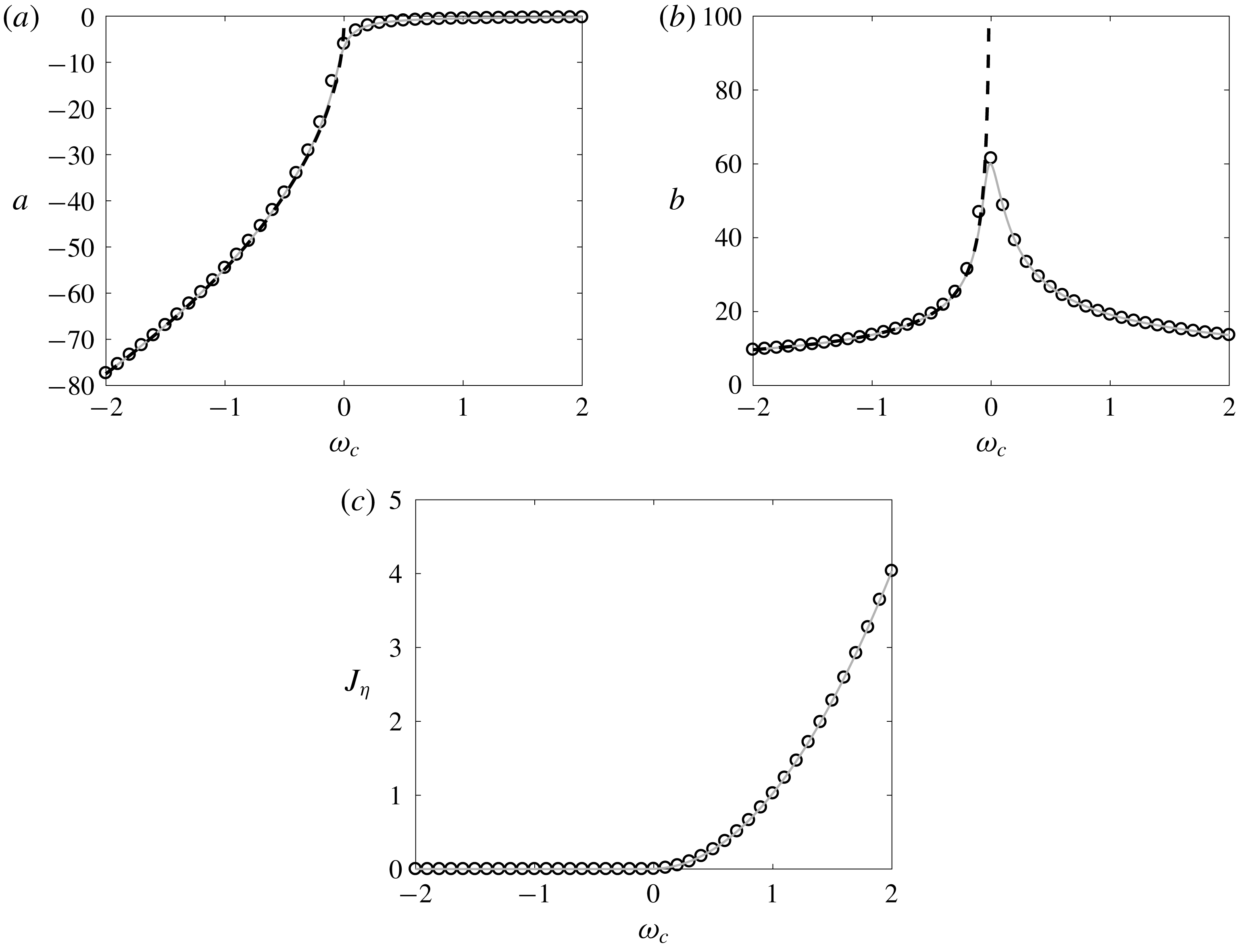
. Figure 8 shows that the predicted values of the optimal values of parameters
 $a$
and
 $b$
closely match both the asymptotic approximations (for
 $\unicode[STIX]{x1D714}_{c}<0$
), and the values obtained from fitting the numerically computed modes. The width parameter for this fit to the numerically computed mode data is found by fitting a Gaussian function to the amplitude of the computed mode using MATLAB’s fit command. The phase parameter is found by considering the gradient of the phase in a small region near the critical layer location. The predicted shape parameters are obtained from evolving the equations (4.22) and (4.23) from an initial condition obtained by solving (4.20) and (4.21) directly (at
 $\unicode[STIX]{x1D714}_{c}=0$
). Here, and in subsequent sections, such solutions (along with the symbolic computation of integrals) are obtained using Mathematica. Note that one could also use the asymptotic approximation given in (4.9) for initial conditions, where we must start from a sufficiently large negative value of
 $\unicode[STIX]{x1D714}_{c}$
to ensure that the initial conditions are accurate. It is additionally shown that the value of the cost function
 $J_{{\mathcal{T}}}$
for these optimal shape parameters closely matches the value of the cost function that may be computed directly from the numerically computed singular value. In essence, this shows that the optimal mode and amplification across all functions is closely approximated by the optimal over the class of functions of the form given in (4.10).
To give a sense for the computational cost of computing the various quantities plotted in figure 8, the numerical svd for the 41
 $\unicode[STIX]{x1D714}$
values plotted took a total of 3.29 s using MATLAB on a laptop computer (with 201 Chebyshev collocation points). Solving (4.20) and (4.21) for a single value of
 $\unicode[STIX]{x1D714}$
with Mathematica took 0.073 s with Mathematica, and evolving the differential equations (4.22) and (4.23) to obtain
 $a(\unicode[STIX]{x1D714})$
and
 $b(\unicode[STIX]{x1D714})$
over the range plotted in figure 8 took 0.067 s. Here we are only considering a one-dimensional parameter space of solutions at a relatively small
 $R$
value, making the direct computation of the leading resolvent modes easy. Nevertheless, the computational advantage of the proposed analytic approximation approach is still apparent.
Prediction of optimal shape parameters (a)
 $a$
and (b)
 $b$
as a function of
 $\unicode[STIX]{x1D714}_{c}=\text{Im}(\unicode[STIX]{x1D706})$
for the leading resolvent modes of the model operator
 ${\mathcal{T}}$
with
 $R=3000$
using both the truncated asymptotic Airy function approximation ((4.9), dashed lines) and minimising the cost function given in (4.19) (grey solid lines), in comparison to values fitted to numerically computed eigenfunctions on a finite domain (circles). (c) Compares the cost function value to the true value (
 $\unicode[STIX]{x1D70E}_{1}^{-2}$
) obtained from the resolvent norm.

We may also consider the behaviour of the optimal shape parameters as
 $R$
varies. Keeping
 $\unicode[STIX]{x1D714}_{c}$
constant, from (4.20)–(4.21) we obtain
 $$\begin{eqnarray}\displaystyle & \displaystyle \frac{\unicode[STIX]{x2202}a}{\unicode[STIX]{x2202}R}=\frac{(1+2\unicode[STIX]{x1D714}_{c}a)R^{3}+4a(a^{2}+3b)R^{2}+12b^{3}R-96a^{3}b^{3}}{2R(\unicode[STIX]{x1D714}_{c}R^{3}+3(a^{2}+b)R^{2}+12\unicode[STIX]{x1D714}_{c}b^{3}R+36b^{3}(b-a^{2}))}, & \displaystyle\end{eqnarray}$$
 $$\begin{eqnarray}\displaystyle & \displaystyle \frac{\unicode[STIX]{x2202}b}{\unicode[STIX]{x2202}R}=\frac{4b^{3}(\unicode[STIX]{x1D714}_{c}^{2}R^{2}+3R(-a+\unicode[STIX]{x1D714}_{c}a^{2}+9\unicode[STIX]{x1D714}_{c}b)+6a^{4}+18b^{2})}{R(\unicode[STIX]{x1D714}_{c}R^{3}+3(a^{2}+b)R^{2}+12\unicode[STIX]{x1D714}_{c}b^{3}R+36b^{3}(b-a^{2}))}. & \displaystyle\end{eqnarray}$$
In the limit of large
 $R$
and for
 $\unicode[STIX]{x1D714}_{c}\neq 0$
(and assuming restrictions on the growth of
 $a$
and
 $b$
with
 $R$
) we have the approximations
 $$\begin{eqnarray}\displaystyle & \displaystyle \frac{\unicode[STIX]{x2202}a}{\unicode[STIX]{x2202}R}\approx \frac{1+2\unicode[STIX]{x1D714}_{c}a}{2\unicode[STIX]{x1D714}_{c}R}, & \displaystyle\end{eqnarray}$$
 $$\begin{eqnarray}\displaystyle & \displaystyle \frac{\unicode[STIX]{x2202}b}{\unicode[STIX]{x2202}R}\approx \frac{4b^{3}\unicode[STIX]{x1D714}_{c}}{R^{2}}, & \displaystyle\end{eqnarray}$$
which we may integrate to infer the scalings
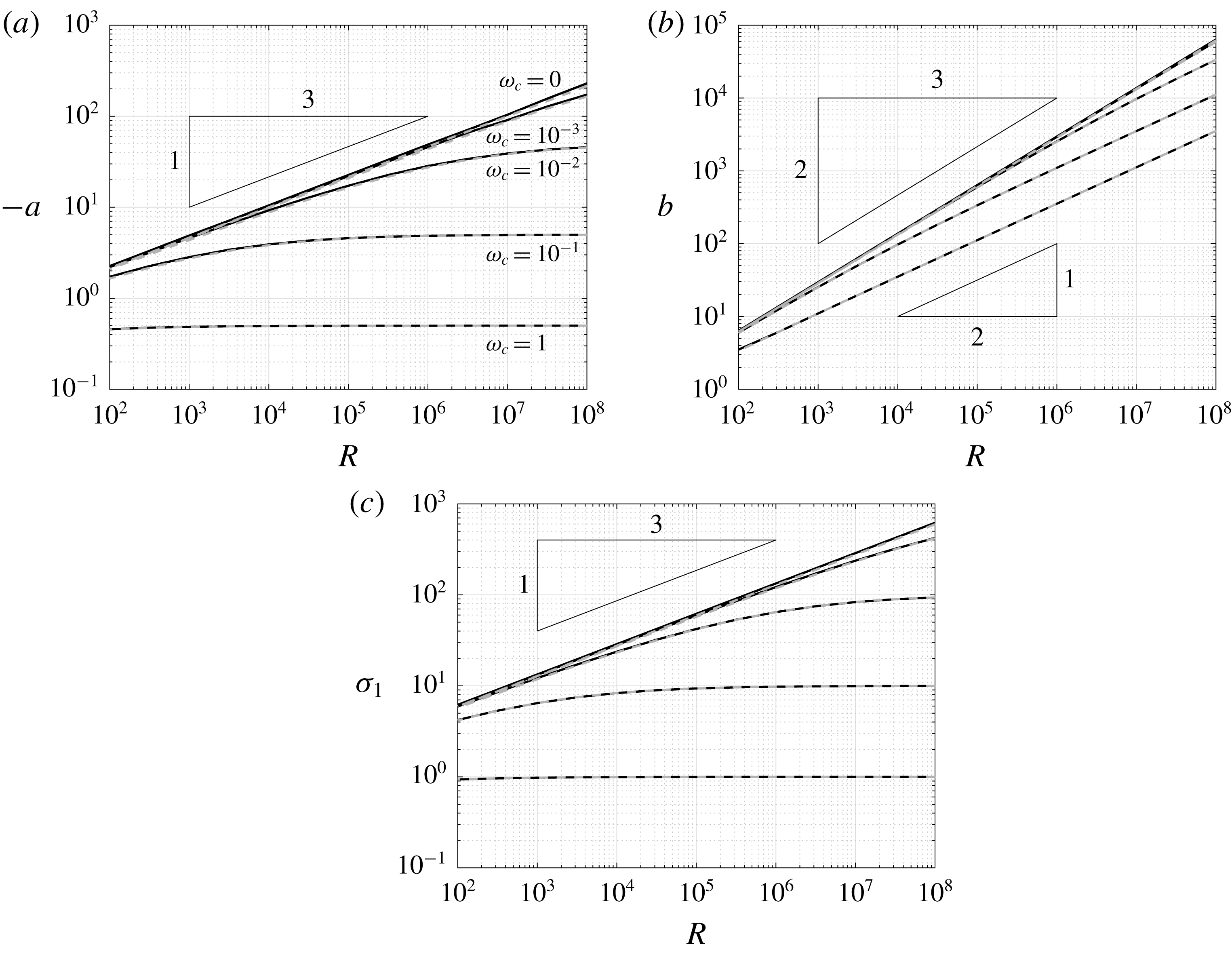
 $a\approx C_{R}R-(2\unicode[STIX]{x1D714}_{c})^{-1}$
and
 $b\propto R^{1/2}$
. For large
 $R$
but with
 $R\unicode[STIX]{x1D714}_{c}\ll 1$
, we instead obtain
 $$\begin{eqnarray}\displaystyle & \displaystyle \frac{\unicode[STIX]{x2202}a}{\unicode[STIX]{x2202}R}\approx \frac{1}{3(a^{2}+b)}, & \displaystyle\end{eqnarray}$$
 $$\begin{eqnarray}\displaystyle & \displaystyle \frac{\unicode[STIX]{x2202}b}{\unicode[STIX]{x2202}R}\approx -\frac{4ab^{3}}{R^{2}(a^{2}+b)}, & \displaystyle\end{eqnarray}$$
which can be shown to permit a consistent asymptotic solution with
 $a\propto R^{1/3}$
and
 $b\propto R^{2/3}$
. This scaling of
 $b$
corresponds to a mode with that scales with
 $R^{1/3}$
, which agrees with the critical layer scaling (Drazin & Reid Reference Drazin and Reid2004), and can also be inferred from the transformation described in (4.4). Figure 9 shows that these scalings closely match the shape parameter trends obtained from the numerically computed modes. Moreover, these shape parameters are accurately predicted from finding optimal parameters of cost function
 $J_{{\mathcal{T}}}$
, which can be obtained either from solving (4.20) and (4.21) for each
 $\unicode[STIX]{x1D714}_{c}$
and
 $R$
, or by evolving the differential equations (4.24) and (4.25) over
 $R$
. Note that the coefficient
 $C_{R}$
that arises from solving (4.26) is very small for the parameters considered here, so
 $a$
appears to approach the constant
 $(2\unicode[STIX]{x1D714}_{c})^{-1}$
in figure 9(a). It should be noted that, even for this model system, computing the leading resolvent modes directly can require substantial computational resources for large
 $R$
(as many collocation points are required to resolve modes with large
 $b$
values, which are highly concentrated around the critical layer), highlighting an advantage of approximations using the methods described in this section. In particular, we used up to 5001 collocation points to compute modes at the highest
 $R$
values considered in figure 9 (although the numerical method could potentially be made more efficient by choosing a discretisation scheme that concentrated collocation points about the critical layer). This resulted in a total cost to compute leading resolvent modes (again using MATLAB on a laptop) for the data plotted in figure 9 (at 13 logarithmically spaced
 $R$
-values) of 2285 s. Solving (4.20) and (4.21) directly for each of these
 $R$
and
 $\unicode[STIX]{x1D714}$
values took a total time of 12.2 s, while computing initial conditions and evolving the differential equations (4.24) and (4.25) took only 0.335 s. This highlights the computational advantage of using a method to approximate mode shapes that does not require the formation and decomposition of large discretised operators.
Comparison between predicted (grey dashed lines) and fitted (solid) parameters (a)
 $a$
and (b)
 $b$
, and (c) associated singular value as a function
 $R$
for the leading resolvent modes of the model operator
 ${\mathcal{T}}$
.

We lastly note that one could seek alternative parameterisations of the two-dimensional space of optimal mode shapes, such as by varying
 $R$
while keeping
 $\unicode[STIX]{x1D714}_{c}R$
(
 $=k_{\bot }^{2}$
) constant.
5 Predicting mode shapes for Navier–Stokes systems
This section extends the analysis of § 4 to predict the shape of resolvent modes for the incompressible Navier–Stokes operator, focusing in particular on the wall-normal vorticity component. We first extend the analysis of § 4 to the Navier–Stokes operator in 5.1, using the approximations presented in § 3.2. We will validate our method first on laminar Couette flow with a linear velocity profile in § 5.1, before returning to the turbulent boundary layer configuration in § 5.2.
5.1 Predicting the shape of resolvent modes for laminar Couette flow
In this section, we will extend the analysis in § 4.2 to consider the Navier–Stokes operator and suboperators considered in §§ 3.1 and 3.2. We again will restrict our attention to predicting the vorticity component of the leading response mode of the resolvent operators
 ${\mathcal{H}}_{\boldsymbol{k}}$
,
 ${\mathcal{H}}_{os,\boldsymbol{k}}$
and
 ${\mathcal{H}}_{sq,\boldsymbol{k}}$
. For the Squire suboperator, the analysis is almost identical to that of the model operator considered in § 4.2. To predict the mode shapes of the full system, we rely on the fact that the response is dominated by the effect of the OS suboperator, which we analyse using the simplifying approximations introduced in § 3.2. In particular, this also results in a methodology similar to that used in § 4.2, but with a modification to use the Laplacian scalar inner product (3.6).
We begin by again assuming mode shapes of the form
 $$\begin{eqnarray}\displaystyle & \displaystyle \unicode[STIX]{x1D713}_{sq}(y)=c_{sq}\exp (\text{i}a_{sq}y-b_{sq}y^{2}), & \displaystyle\end{eqnarray}$$
 $$\begin{eqnarray}\displaystyle & \displaystyle \unicode[STIX]{x1D713}_{os}(y)=c_{os}\exp (\text{i}a_{os}y-b_{os}y^{2}), & \displaystyle\end{eqnarray}$$
but now to satisfy the unit-norm requirements of the relevant inner products ((3.5) for the SQ operator, equation (3.6) for the OS) we have
 $$\begin{eqnarray}\displaystyle c_{sq}=\left(\frac{2b_{sq}}{\unicode[STIX]{x03C0}}\right)^{1/4}k_{\bot },\quad c_{os}=\left(\frac{2b_{os}}{\unicode[STIX]{x03C0}}\right)^{1/4}k_{\bot }(b_{os}+a_{os}^{2}+k_{\bot }^{2}), & & \displaystyle\end{eqnarray}$$
where, with reference to the previous section, we have
 $k_{\bot }^{2}=\unicode[STIX]{x1D714}_{c}R$
. Using the approximation to the Orr–Sommerfeld operator introduced in § 3.2, and noting that
 $U_{y_{c}}=1$
, the relevant cost functions for optimising the shape of the SQ and OS template functions are
 $$\begin{eqnarray}\displaystyle \displaystyle J_{sq}(a,b;R,\boldsymbol{k})=\Vert U_{y_{c}}k_{x}{\mathcal{T}}\unicode[STIX]{x1D713}_{sq}\Vert ^{2} & = & \displaystyle \frac{U_{y_{c}}^{2}k_{x}^{2}}{k_{\bot }^{2}}\int _{y=-\infty }^{\infty }({\mathcal{T}}\unicode[STIX]{x1D713}_{sq})^{\ast }({\mathcal{T}}\unicode[STIX]{x1D713}_{sq})\,\text{d}y,\end{eqnarray}$$
 $$\begin{eqnarray}\displaystyle \displaystyle J_{os}(a,b;R,\boldsymbol{k})=\Vert U_{y_{c}}k_{x}{\mathcal{T}}\unicode[STIX]{x1D713}_{os}\Vert _{\unicode[STIX]{x1D6E5}}^{2} & = & \displaystyle \frac{U_{y_{c}}^{2}k_{x}^{2}}{k_{\bot }^{2}}\int _{y=-\infty }^{\infty }({\mathcal{T}}\unicode[STIX]{x1D713}_{os})^{\ast ,\unicode[STIX]{x1D6E5}}({\mathcal{T}}\unicode[STIX]{x1D713}_{os})\,\text{d}y\nonumber\\ \displaystyle & = & \displaystyle -\frac{U_{y_{c}}^{2}k_{x}^{2}}{k_{\bot }^{2}}\int _{y=-\infty }^{\infty }({\mathcal{T}}\unicode[STIX]{x1D713}_{os})^{\ast }\unicode[STIX]{x1D6E5}({\mathcal{T}}\unicode[STIX]{x1D713}_{os})\,\text{d}y.\end{eqnarray}$$
For laminar Couette flow we have
 $U_{y_{c}}=1$
for all
 $y_{c}$
in the domain, but we keep this term so that the equations are directly applicable for arbitrary mean velocity profiles. Also note that while the cost function for the Squire modes is ‘exact’ given the assumed template function and a linear mean velocity profile, the OS modes are relying on the accuracy of a simplified operator (being the scalar Squire operator with a Laplacian inner product) capturing the correct behaviour of the response mode.
Substituting in the mode template functions (and dropping the subscripts on
 $a$
and
 $b$
parameters for brevity), explicit expressions for the cost functions are
 $$\begin{eqnarray}\displaystyle \displaystyle J_{sq}(a,b;R,\boldsymbol{k}) & = & \displaystyle \frac{U_{y_{c}}^{2}k_{x}^{2}}{k_{\bot }^{2}}\left[\frac{1}{4b}+\frac{3}{R^{2}}b^{2}+\frac{2(3a^{2}+k_{\bot }^{2})}{R^{2}}b+\frac{a^{4}+2aR+2k_{\bot }^{2}a^{2}+k_{\bot }^{4}}{R^{2}}\right],\end{eqnarray}$$
 $$\begin{eqnarray}\displaystyle \displaystyle J_{os}(a,b;R,\boldsymbol{k}) & = & \displaystyle \frac{U_{y_{c}}^{2}k_{x}^{2}}{4k_{\bot }^{2}b(b+a^{2}+k_{\bot }^{2})R^{2}} [(3b+a^{2}+k_{\bot }^{2})R^{2}+16ab(3b+a^{2}+k_{\bot }^{2})R\nonumber\\ \displaystyle & & \displaystyle +\,4b(15b^{3}+(a^{2}+k_{\bot }^{2})^{3}+9b^{2}(5a^{2}+k_{\bot }^{2})+3b(a^{2}+k_{\bot }^{2})(5a^{2}+k_{\bot }^{2}))].\nonumber\\ \displaystyle & & \displaystyle\end{eqnarray}$$
As before, the minima of these cost functions may be found by selecting the appropriate solution to the equations
 $$\begin{eqnarray}\displaystyle & \displaystyle \frac{\unicode[STIX]{x2202}J_{sq}}{\unicode[STIX]{x2202}a}=\frac{2U_{y_{c}}^{2}k_{x}^{2}}{k_{\bot }^{2}R^{2}}(6ab+2a^{3}+2k_{\bot }^{2}a+R)=0, & \displaystyle\end{eqnarray}$$
 $$\begin{eqnarray}\displaystyle & \displaystyle \frac{\unicode[STIX]{x2202}J_{sq}}{\unicode[STIX]{x2202}b}=\frac{U_{y_{c}}^{2}k_{x}^{2}}{k_{\bot }^{2}}\left[-\frac{1}{4b^{2}}+\frac{2}{R^{2}}(3b+3a^{2}+k_{\bot }^{2})\right]=0, & \displaystyle\end{eqnarray}$$
 $$\begin{eqnarray}\displaystyle \frac{\unicode[STIX]{x2202}J_{os}}{\unicode[STIX]{x2202}a} & = & \displaystyle \frac{U_{y_{c}}^{2}k_{x}^{2}}{k_{\bot }^{2}(b+a^{2}+k_{\bot }^{2})^{2}}\left[-a+\frac{4}{R}(3b^{2}+4k_{\bot }^{2}b+(a^{2}+k_{\bot }^{2})^{2})\right.\nonumber\\ \displaystyle & & \displaystyle \left.+\,\frac{4a}{R^{2}}(15b^{3}+9b(a^{2}+k_{\bot }^{2})^{2}+(a^{2}+k_{\bot }^{2})^{3}+3b^{2}(5a^{2}+9k_{\bot }^{2}))\right]=0,\end{eqnarray}$$
 $$\begin{eqnarray}\displaystyle \frac{\unicode[STIX]{x2202}J_{os}}{\unicode[STIX]{x2202}b} & = & \displaystyle \frac{U_{y_{c}}^{2}k_{x}^{2}}{k_{\bot }^{2}(b+a^{2}+k_{\bot }^{2})^{2}}\left[-\frac{3}{4}-\frac{1}{2b}(a^{2}+k_{\bot }^{2})-\frac{1}{b^{2}}(a^{2}+k_{\bot }^{2})^{2}+\frac{8}{R}a(a^{2}+k_{\bot }^{2})\right.\nonumber\\ \displaystyle & & \displaystyle +\,\frac{2}{R^{2}} (15b^{3}+(a^{2}+k_{\bot }^{2})^{2}(7a^{2}+k_{\bot }^{2})+9b^{2}(5a^{2}+3k_{\bot }^{2})\nonumber\\ \displaystyle & & \displaystyle \left.+\,9b(5a^{2}+k_{\bot }^{2})(a^{2}+k_{\bot }^{2}))\right]\nonumber\\ \displaystyle & = & \displaystyle 0.\end{eqnarray}$$
Figure 10 compares the predicted shape parameters to those obtained from fitting these parameters to numerically computed modes, which are computed for
 $Re=1000$
and various values of
 $k_{x}$
and
 $k_{z}/k_{x}$
. We observe in panels (a) and (c) that the Squire mode parameters are accurately predicted from solving (5.8) and (5.9). Panels (b) and (d) show that solving (5.10) and (5.11) predicts the fitted parameters to the leading resolvent response mode of the Squire operator with Laplacian inner product. Furthermore, this prediction also accurately predicts the shape of the wall-normal vorticity component of leading response modes for the full Navier–Stokes system. Note that the scaling laws for small
 $k_{x}$
are identical to those for small
 $R$
observed in figure 9. The trends at high
 $k_{x}$
differ from those in figure 9, due to the fact that here we keep
 $k_{z}$
proportional to
 $k_{x}$
(and thus
 $k_{\bot }\propto R$
), whereas in figure 9 constant
 $\unicode[STIX]{x1D714}_{c}$
resulted in
 $k_{\bot }^{2}\propto R$
. These trends can again be inferred from studying the dominant terms in the evolution equations for the governing parameters, which can be computed from considering the partial derivatives of
 $J_{sq}$
and
 $J_{os}$
with respect to
 $a$
and
 $b$
, which we omit for brevity.
Comparison between predicted (grey solid lines) and fitted (circles) mode shape parameters
 $a$
(a,b) and
 $b$
(c,d) for the Squire operator with a standard (a,c) and Laplacian (b,d) inner product, as a function of streamwise wavenumber
 $k_{x}$
, for
 $Re=1000$
and spatial aspect ratios
 $k_{z}/k_{x}\in \{0.5,1,2,4,8\}$
. Also shown are fitted shape parameters for the
 $\unicode[STIX]{x1D702}$
-component of the full Navier–Stokes system (red crosses).

For large
 $k_{x}$
, the mode shapes for both operators converge, which may be explained by the fact that the Laplacian operator is dominated by the constant
 $k_{\bot }^{2}$
term in this regime. As a consequence, here analysis of the Squire operator gives accurate predictions of the behaviour of the full Navier–Stokes system, particularly for the mode width, which approaches a constant value with increasing
 $k_{x}$
. There is some difference between the phase gradient parameter
 $a$
for the full system and for the Squire system with both the standard and Laplacian inner product (with the value for the full system lying between those for the two simplified systems), although this difference decreases as
 $k_{x}$
increases and the phase variation decays towards zero.
Comparison between true (numerically computed, solid lines) and predicted (orange dotted) mode amplitudes for laminar Couette flow with
 $Re=1000$
and
 $k_{x}=1$
(a,b) 10 (c,d) and 100 (e,f), and aspect ratios
 $k_{z}/k_{x}\in \{0.5,1,2,4,8\}$
. Panels (a,c,e) show results for the Squire subsystem, while (b,d,f) are for the Navier–Stokes operator. Numerically computed mode amplitudes for the Orr–Sommerfeld subsystem are also shown (blue dashed) in (b,d,f).

Figure 11 plots predicted and true mode amplitudes for several of the cases considered in figure 10. The predicted mode shapes for
 $\unicode[STIX]{x1D702}$
closely match the computed modes for both the Squire and full Navier–Stokes system, with the modes for the latter being very close to those of the OS subsystem. The largest discrepancy arises in the
 $k_{x}=1$
case, where the tails of the mode amplitudes are significantly heavier than those of a Gaussian distribution, and extend far from the critical layer towards the wall. This phenomenon is related to a wider distribution in the
 $v$
-component of the mode (not plotted), and gives a larger variation in fitted
 $b$
values for this
 $k_{x}$
for the full Navier–Stokes system, as observed in figure 10.
(a) Projection error between numerically computed and predicted modes for the Squire subsystem with regular (grey dashed) and Laplacian (blue solid) inner products, and the full Navier–Stokes system (red dotted) for laminar Couette flow. (b) Comparison between predicted and computed leading singular values for the Squire subsystem with regular (predicted grey dashed, computed crosses) and Laplacian (predicted solid blue, computed circles) inner product. Also shown are computed singular values for the full Navier–Stokes system (red dotted). All parameters are the same as those in figure 10.

To quantify the quality of the mode shape approximations, we plot in figure 12(a) the projection error between the true (numerically computed,
 $\unicode[STIX]{x1D713}_{\unicode[STIX]{x1D702},true}$
) and predicted (
 $\unicode[STIX]{x1D713}_{\unicode[STIX]{x1D702},pred}$
) mode shapes, given by
 $$\begin{eqnarray}\displaystyle \unicode[STIX]{x1D716}=1-\langle \unicode[STIX]{x1D713}_{\unicode[STIX]{x1D702},true},\unicode[STIX]{x1D713}_{\unicode[STIX]{x1D702},pred}\rangle , & & \displaystyle\end{eqnarray}$$
where both
 $\unicode[STIX]{x1D713}_{\unicode[STIX]{x1D702},true}$
and
 $\unicode[STIX]{x1D713}_{\unicode[STIX]{x1D702},pred}$
are assumed to have unit norm. We observe that
 $\unicode[STIX]{x1D716}<0.01$
for all cases, with the error generally tending to decrease for higher wavenumbers (where the modes become more concentrated about the critical layer), particularly for the Squire subsystem. Larger errors are observed at around
 $k_{x}=1$
for both the Navier–Stokes system and the Squire subsystem with a Laplacian inner product. This can be attributed to the non-Gaussian ‘heavy tails’ on these modes that can be observed in figure 11(b). There is also larger error for the Navier–Stokes system at
 $k_{x}\approx 30$
(particularly for lower
 $k_{z}/k_{x}$
values), which can be attributed to (relatively small) errors in the prediction of the correct
 $b$
value in this regime (which can be just discerned in figure 10
d). Note also that since we interpolate onto the computational grid when computing this error, we are not accounting for the error associated with estimated modes being non-zero outside of the computational domain. This could lead to slight underestimates of the error at small spatial wavenumbers.
Figure 12(b) compares the leading resolvent singular values for the Squire and Navier–Stokes systems to those estimated from the minima of the cost functions
 $J_{sq}$
and
 $J_{os}$
, for the same wavenumbers considered in figure 10. The cost functions are able to accurately predict the singular values of the scalar Squire operator with both the regular and Laplacian inner product, although this is only accurate for the full Navier–Stokes system for large
 $k_{x}$
(and thus large
 $k_{\bot }^{2}$
). In particular, these model operators are incapable of predicting the increase in singular value for high-aspect-ratio (i.e. large
 $k_{z}/k_{x}$
) modes that is observed, although we have shown that they still accurately predict mode shapes in this regime. This is perhaps unsurprising, since the analysis in § 3.2 predicts that the Squire operator with a Laplacian inner product can predict the resolvent response mode, but does not say anything about finding the correct singular value.
5.2 Predicting mode shapes for a turbulent boundary layer
This section applies the methodology developed in §§ 4.2 and 5.1 to the incompressible turbulent boundary layer system introduced in § 3. By linearising the mean velocity profile about the critical layer, the equations for predicting mode shape parameters are the same as those developed in § 5.1 (i.e. (5.6)–(5.11)), although now
 $U_{y_{c}}$
and
 $R=k_{x}U_{y_{c}}Re$
are dependent on the critical layer location. Figure 13 shows the predicted and true response mode shapes for the Squire and Navier–Stokes resolvent operators for two pairs of spatial wavenumbers and various critical layer locations. Note that the case where
 $\{k_{x},k_{z},c\}=\{\unicode[STIX]{x03C0}/2,2\unicode[STIX]{x03C0},0.8U_{\infty }\}$
as considered in figures 1–3 as representative of a typical large-scale motion, is included. The location typical of very-large-scale motions (
 $c\approx 0.6U_{\infty }$
) is also included, although these structures would correspond to slightly smaller streamwise wavenumbers than
 $k_{x}=\unicode[STIX]{x03C0}/2$
. We observe that mode amplitude and phase variation (in the local region of high amplitude) is accurately estimated, provided the mode is not substantially affected by the presence of the wall. Note in particular that the predicted mode shapes will only ever approximately satisfy the boundary conditions at the wall, and this approximation is only accurate for cases where the true modes are themselves ‘detached’ from the wall. Aside from this issue, the general agreement between the true and predicted mode shapes shows in particular the validity of using a mean velocity profile linearised about the critical layer to estimate mode shapes.
True (solid blue lines) and predicted (red dashed) leading resolvent mode amplitudes (a,c,e,g) and phases (b,d,f,h) for the Squire system (a–d) and wall-normal vorticity component of the Navier–Stokes system (e–h) for a turbulent boundary layer with
 $Re_{\unicode[STIX]{x1D70F}}=900$
. Modes are shown for two wavenumber pairs,
 $(k_{x},k_{z})=(\unicode[STIX]{x03C0}/2,2\unicode[STIX]{x03C0})$
(a,b,e,f) and
 $(10\unicode[STIX]{x03C0},10\unicode[STIX]{x03C0})$
(c,d,g,h), and temporal frequencies corresponding to wave speeds of
 $0.6U_{\infty }$
,
 $0.7U_{\infty }$
,
 $0.8U_{\infty }$
,
 $0.9U_{\infty }$
, with critical layer locations indicated by dotted lines.

As was the case for the model operator considered in § 4, we again find that the analytic method requires substantially less computational time. For the modes shown in figure 13, the analytic mode shape predictions required 0.34 s for the Squire modes (obtained by solving (5.8) and (5.9)), and 22.4 s for the prediction of the
 $\unicode[STIX]{x1D702}$
-component of the wall-normal vorticity component of the Navier–Stokes system (5.10) and (5.11). In comparison, the numerical modes (computed using 801 collocation points) took 97.5 s and 150 s for the Squire and Navier–Stokes systems respectively.
To study the performance of our proposed method for a turbulent boundary layer further, figure 14 compares predicted and fitted mode shape parameters as a function of
 $k_{x}$
for various aspect ratios
 $k_{z}/k_{x}$
, for a wave speed
 $c=0.8U_{\infty }$
, with predicted and true modes shapes plotted in figure 15. We observe the same trends, and similar accuracy in prediction of parameters as for laminar Couette flow (figure 10).
The primary difference between the laminar Couette flow example and the turbulent boundary layer is that the latter relies upon the accuracy of the local linearisation of the mean velocity field (since the former has a linear mean velocity profile to begin with). The overall similarity between the results for the turbulent boundary layer suggests that this approximation is generally reasonable and justified.
Comparison between predicted (solid grey lines) and fitted (circles) mode shape parameters
 $a$
(a,b) and
 $b$
(c,d) for the Squire operator with a standard (a,c) and Laplacian (b,d) inner product, as a function of streamwise wavenumber
 $k_{x}$
, for various mode aspect ratios for a turbulent boundary layer with
 $Re_{\unicode[STIX]{x1D70F}}=900$
and
 $c=0.8U_{\infty }$
. Also shown are fitted shape parameters for the
 $\unicode[STIX]{x1D702}$
component of the full Navier–Stokes system (red crosses).

Comparison between true (numerically computed, solid lines) and predicted (orange dotted) mode amplitude for incompressible turbulent boundary layer flow with
 $Re_{\unicode[STIX]{x1D70F}}=900$
and
 $k_{x}=1$
(a,b) 10 (c,d) and 100 (e,f), and aspect ratios
 $k_{z}/k_{x}\in \{0.5,1,2,4,8\}$
. Panels (a,c,e) show results for the Squire subsystem, while (b,d,f) are for the Navier–Stokes operator. Numerically computed mode amplitudes for the Orr–Sommerfeld subsystem are also shown (blue dashed) in (b,d,f).

(a) Projection error between numerically computed and predicted modes for the Squire subsystem with regular (grey dashed lines) and Laplacian (blue solid) inner products, and the full Navier–Stokes system (red dotted) for a turbulent boundary layer with
 $Re_{\unicode[STIX]{x1D70F}}=900$
and
 $c=0.8U_{\infty }$
. (b) Comparison between predicted and computed leading singular values for the Squire subsystem with regular (predicted grey dashed, computed crosses) and Laplacian (predicted blue solid, computed blue circles) inner product. Also shown are computed singular values for the full Navier–Stokes system (red dotted). All parameters are the same as those in figure 14.

Figure 16(a) shows the projection error (5.12) between the true and predicted mode shapes for the turbulent boundary layer, for the same parameters considered in figure 14. We observe some similar trends observed in figure 12(a) for laminar Couette flow, but significantly larger errors at low
 $k_{x}$
values for both the full system, and for the Squire operator with Laplacian inner product. These large errors can be attributed to two causes, both related to the increasing width of modes as
 $k_{x}$
decreases. First, the wall starts to affect the shape of these modes, and second, the local linearisation of the mean velocity profile becomes less valid. Both of these effects can be observed in figure 15(b), where large discrepancies are observed both near the wall, and towards the outer edge of the boundary layer. In general, however, this quantification of error shows that our mode shape approximation accurately captures the dominant features of numerically computed resolvent modes across a wide range of wavenumbers.
Figure 16(b) plots numerically computed and predicted singular values for this system. As was the case with laminar Couette flow, our methods are able to predict the leading singular values of the Squire operator with the standard and Laplacian inner products, but not those for the full Navier–Stokes operator at low values of
 $k_{x}$
(which can again be attributed to the fact that our approximations are not designed to capture the gain of the full Navier–Stokes operator in all regimes).
6 Discussion and conclusions
This work has presented a method for approximating leading resolvent response modes for quasi-parallel shear-driven flows. This method relies on the assumption that the true mode may be closely approximated by a simple template function, the general form of which can be reasoned from consideration of wavepacket pseudomode theory. In essence, the method reduces the space of possible mode shapes from an infinite-dimensional space (which in practice is approximated by a high-dimensional space defined by the numerical discretisation) to a two-dimensional family of functions. Once this template function is identified, the optimal shape parameters (which govern the width and phase variation of the mode) may be found as the minimisers of a cost function, which is directly related to the resolvent norm of the underlying operator. In practice, this amounts to finding the roots of a pair of coupled equations, which may be arranged to be polynomials in the shape parameters. In addition, it is possible to derive differential equations in parameter space that govern the evolution of these optimal shape parameters. Importantly, this method precludes the need for the formulation and decomposition of discretised linear operators, leading to substantial reduction in computational cost. The extent of the reduction in computational cost is dependent on the size of the discretisation, and on the extent and resolution of the parameter space (e.g. wavenumbers and temporal frequencies) that one wishes to study, and the method used (i.e. solving for the roots of the polynomials directly for each parameter set of interest, or evolving the associated differential equations numerically in parameter space). In this work, we have found computational speedup by factors ranging from around 10 to 1000, depending on these aforementioned parameters. Note that this computational speed up could be particularly advantageous for the real-time estimation of and control of highly amplified structures, if using a model based on the resolvent framework.
The methods developed in this work may be readily applied to a model operator, as considered in § 4.2, and in the analysis of the Squire operator in §§ 5.1–5.2. Application for the full Navier–Stokes system relies on additional simplifications to arrive at a scalar differential operator which has a leading response mode (left singular vector) which approximates the wall-normal vorticity component of the response mode of the Navier–Stokes resolvent operator, as detailed in § 3.2. This simplification is made in three steps. Firstly, the observation that the wall-normal vorticity response is dominated by the Orr–Sommerfeld component (3.9). Secondly, that this operator is in turn dominated by the vorticity response to velocity forcing, governed by the scalar operator (3.12). Finally, the leading left singular vector of this scalar operator may be approximated by that of the Squire operator furnished with the scalar Laplacian inner product (3.6). This results in an operator which may be studied by applying the same techniques as those used for the model/Squire system. As well as making our analysis tractable, this last step forms an explicit connection between the Orr mechanism (as governed by the Squire operator) and the lift-up mechanism (which is directly associated with the Orr–Sommerfeld operator), by showing that these two mechanisms can be related to the same operator with an appropriate choice of inner product.
While the vorticity response mode shapes of the Squire and Orr–Sommerfeld resolvent operators are qualitatively similar, they represent quite different physical phenomena. The Squire resolvent operator describes amplification through forcing in the same component, with an upstream-leaning optimal forcing mode giving a downstream-leaning response mode, which is a manifestation of the classical Orr mechanism. Note in particular that the Squire forcing mode has the same amplitude profile as the response mode, but with an opposite phase variation. The Orr–Sommerfeld sub-operator on the other hand typically has a leading response mode that is dominated by the wall-normal vorticity component, but is forced primarily by wall-normal velocity, in a manner resembling the lift-up mechanism. Despite this phenomenological difference, we have shown that the shape of the response may be accurately predicted from the Squire operator with a modified inner product.
Note that, even without this analysis, study of the Squire operator (for which the associated cost function has a simpler form) typically gives the same qualitative behaviour observed for the full system. In particular, the Squire system obeys many of the same scaling laws of mode shape parameters with wavenumbers and Reynolds numbers. More detailed analysis of scaling and self-similarity properties of resolvent modes in wall-bounded flows are given in Moarref et al. (Reference Moarref, Sharma, Tropp and McKeon2013).
This work has focused on characterising the shape of the (dominant) wall-normal vorticity component resolvent modes for incompressible quasi-parallel wall-bounded flows. It is possible that these methods could be extended for application to more complex geometries, and other mode components. Here we have explicitly tested our method for a turbulent boundary layer profile, but the same methodology should extend to other quasi-parallel shear flows. For example, we have also tested the method on both laminar and turbulent channel flows. One caveat to this is that care needs to be taken in regions where the wall-normal gradient of the mean velocity is close to zero, since our method relies on the assumption that a first-order Taylor series expansion of the mean velocity field is sufficient to capture the influence of the mean velocity in determining the shape of leading resolvent modes.
For most of the cases considered in this work, the cost function had only one local minimum corresponding to a wavepacket mode (i.e. with
 $b>0$
), with the exception being for negative
 $\unicode[STIX]{x1D714}_{c}$
for the model operator considered in § 4.2. More complex geometries might result in more complex cost functions, for which more care must be taken to select the true global optimum. Note that the operators considered here also typically have a large spectral gap between the first and second singular value, which presumably increases the robustness of the method in correctly identifying the leading mode. Conversely, the existence of these wavepacket pseudospectral modes with high gain could also be viewed as a reason for this large spectral gap, since our method is predicting the existence of a function that almost makes the resolvent operator singular. Future work could also seek to identify modes corresponding to additional singular values, which would be of particular interest for situations where the operator does not exhibit low-rank behaviour (i.e. there does not exist a large gap between the leading and second singular values). For such cases, care would need to be taken to ensure that the correct modes were being identified, and one might also need to extend the method to allow for modes with multiple amplitude peaks, which are empirically observed for higher-order modes. Additionally, the gap between adjacent singular values typically reduces substantially for suboptimal modes, meaning that more care would be required to ensure that the ‘correct’ suboptimal mode was being identified. Similar methods could also be applied to study optimal forcing modes in more detail, and to compute nonlinear forcing terms induced from analytic approximations to wavepacket modes. This would provide an alternative route to study phenomena such as the self-similarity of the nonlinear forcing (Sharma, Moarref & McKeon Reference Sharma, Moarref and McKeon2017).
In terms of the methodology itself, there are a number of possible refinements that could be investigated. For example, nonlinear terms in the expansion of the mean velocity profile about the critical layer could be retained, and additional terms in the template mode function could also be included (for example, a term allowing for the phase variation to be cubic in
 $y-y_{c}$
). The former modification might be particularly useful when dealing with mean velocity profiles that have stationary points, such as in channel flow. Such extensions would still allow for the analytic computation of
 ${\mathcal{T}}\unicode[STIX]{x1D713}$
, and for closed-form expressions for the cost functions in (5.6) and (5.7), since the underlying methods only require the application of differential and integral operations to known analytic functions. The accuracy of the assumed form of the modes relies on the mode being far enough away from the wall, although further extensions of the methodology could seek to explicitly model the effect of the wall.
Acknowledgements
The authors acknowledge support from the Air Force Office of Scientific Research grant FA9550-16-1-0232 (programme manager I. Leyva). The authors also thank P. Schmid, A. Leonard and K. Rosenberg for valuable discussions, and X. Wu for allowing us to use his turbulent boundary layer database. Lastly, the authors thank the anonymous reviewers for numerous helpful suggestions to improve the paper.