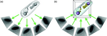


1. Introduction
The science of cell biology has been driven by advances in imaging technologies ever since the discovery of cells by Robert Hooke and Antonie van Leeuwenhoek in the 17th century. As optics improved over the next three centuries, so did our knowledge of cell ultrastructure and function. The development of chromogenic stains enabled the visualization of otherwise ‘invisible’ intracellular bodies, including chromosomes inside the nucleus. In the late 19th century Ernst Abbe recognized, however, that the resolution of light microscopes would ultimately be limited to about half the wavelength of light.
The invention of the electron microscope by Ruska in the early 1930s and the availability of commercial instruments shortly thereafter promised a new era of cell biology in which resolution could be extended by at least two orders of magnitude. Despite this transformative technological advance, the first images of subcellular structures such as ribosomes, viruses and the cytoskeleton were not obtained for approximately two more decades. Some of the principal challenges were that biological specimens are hydrated and radiation sensitive, exhibit poor intrinsic contrast, and are often too thick to be imaged intact. To solve these problems, methods were developed to chemically fix and stain specimens, embed them in plastic resins, and section them with a microtome. Together, these techniques enabled a ‘Golden age’ of rapid discovery in the 1950s to 1960s (Fig. 1).
Timeline of key developments. Key technologies and applications of EM are shown. The gray gradients emphasize that each of these development took many years.

Electron microscopy (EM) images are 2D projections. To gain the perspective of depth, stereoscopy was introduced, in which two images are taken of a specimen – one at positive tilt and the other at negative tilt. The pair of images were viewed with a stereoscope, and quantitative data could be generated by measuring relative displacements of objects perpendicular to the tilt axis and then calculating their separation in ‘Z’ (the direction parallel to the electron beam) using the known tilt angles. But since stereoscopy uses only two views of the specimen, the resolution in Z is limited.
Another way to obtain 3D information is to cut a sample into a series of thin sections and image each section individually. As each section represents a resolution element in Z, an entire cell can then be reconstructed in 3D by computationally stacking the images. Reconstructions from serial sections have an anisotropic resolution of ~1–2 nm in the cutting plane (limited by the stain granularity), but only ⩾20 nm perpendicular to the cutting direction (limited by how thin sections can be cut and handled) (Mastronarde et al. Reference Mastronarde, Ladinsky and Mcintosh2000). Fine structural details of cellular organization are often further obfuscated by the losses that occur on the cutting planes, sample shrinkage and warping caused by radiation damage, and the difficulty of tracking features between sections (especially features that lie in a cutting plane). Nevertheless, since it is relatively straightforward to do in any laboratory with an EM, this method has been used since the 1950s to map out the ultrastructure of various eukaryotic cells and tissues. As an example of the power of this technique, the Caenorhabditis elegans ‘connectome’ – the wiring diagram of all 302 neurons in this millimeter-long worm – was reconstructed by serial EM (White et al. Reference White, Southgate, Thomson and Brenner1986).
A third method to obtain high-resolution ‘3D’ EM images of at least the surface of biological objects is scanning electron microscopy. Newer methods that combine sequential focused-ion beam milling with SEM (also called ion–abrasion scanning electron microscopy) are beginning to reveal internal detail as well, as demonstrated in a recent study of murine liver (Murphy et al. Reference Murphy, Lowekamp, Zerfas, Chandler, Narasimha, Venditti and Subramaniam2010). In this ‘slice-and-scan’ approach, a heavy-metal-stained, plastic-embedded block of cells is imaged on one face by SEM, then milled to expose a fresh surface and imaged again. This ‘sequential imaging’ technique eliminates the distortion artifacts that may occur when adjacent sections are imaged separately for serial-section reconstruction. It is not yet known, however, how deeply the interior of the block can be uniformly stained, milled and imaged, and how this will affect the range of structures that can be examined.
Alternatively, samples can be imaged to a resolution of ~2–8 nm in all three directions without losses or distortions between sections through electron tomography (Fig. 2). Specimens are incrementally tilted in a transmission EM through a range up to ±70° and imaged at each step. Each image in this ‘tilt series’ represents a different view of the specimen. The images are aligned and then ‘back-projected’ to generate a 3D reconstruction or ‘tomogram’, of the specimen. Electron tomography is therefore the highest resolution technique available today to image unique biological specimens such as cells.
Principle of electron tomography. (a) A tilt series of projection images is acquired from the object as it is incrementally tilted. (b) The tomogram is generated by back-projecting the aligned projection images.

In this review, we will summarize the current methods and technologies to prepare a specimen, collect data, generate a tomogram, and finally interpret and analyze the result (for additional technical details, see also Frank, Reference Frank2006; Koster et al. Reference Koster, Grimm, Typke, Hegerl, Stoschek, Walz and Baumeister1997; Lucic et al. Reference Lucic, Forster and Baumeister2005). While electron tomography can be used to image even individual macromolecular complexes (Murphy & Jensen, Reference Murphy and Jensen2005), here we limit ourselves to the application of electron tomography to cells. The role of electron tomography in solving important cell biology problems will then be illustrated with a few example studies of eukaryotic and bacterial ultrastructure and virus-cell interactions.
2. Technology and techniques
2.1 Specimen preparation
EM specimens must satisfy two important requirements to produce useful phase-contrast EM images: they must be stable within the microscope's high vacuum and they must be thin. Since cells are composed mostly of water, their molecular structure must be fixed (mechanically stabilized) somehow before they can be imaged in the microscope. Samples must be thin because while phase contrast arises from the interference between unscattered and elastically scattered electrons, inelastically scattered electrons emerge from the sample with increased wavelengths and therefore focus differently, blurring the image. Inelastically scattered electrons are therefore typically removed from the image with an energy filter. There is no exact limit on how thin a specimen must be, but because the probability of electrons being inelastically scattered increases with sample thickness, and the path length of the electrons through the sample increases with tilt angle α by ~1/cos(α), sample thickness is generally limited to about 200 nm in 100 kV instruments and approximately twice than that in 300 kV instruments. While higher voltage (up to several MeVs) EMs exist, these instruments are extremely rare and only moderately expand (approximately another doubling) the permissible specimen thickness.
The first method that was developed to stabilize a biological specimen is chemical fixation. Cells (or small pieces of tissue) can be fixed at room temperature with cross-linking agents like glutaraldehyde. Next, the cells are typically post-fixed with osmium tetroxide, a cross-linking agent that also serves as a heavy-metal stain. The cells are then dehydrated with an organic solvent such as acetone or ethanol and infiltrated with embedding resin. The resin is polymerized, yielding a mechanically stable ‘block’ of cells which can be subsequently sectioned in a microtome. To enhance the contrast, the cells can be post-stained with a heavy metal salt such as uranyl acetate or lead citrate (usually after microtomy). Because this ‘traditional’ chemical fixation method can be applied to almost any specimen and the samples can be imaged at room temperature in almost any EM, it has been widely used for decades and has generated a vast archive of cellular images. Unfortunately, because fixation occurs in tens of seconds or longer and different parts of cells are fixed at different rates, dynamic cellular structures often disassemble and molecules that do not normally interact can be cross-linked into un-physiological complexes (McDonald & Auer, Reference Mcdonald and Auer2006).
Cellular structures can be better preserved if they are quickly frozen. Crystalline ice, however, can damage proteins and can generate image artifacts when the diffraction condition is satisfied (Dubochet et al. Reference Dubochet, Adrian, Chang, Homo, Lepault, Mcdowall and Schultz1988). A family of techniques have therefore been developed to rapidly cool cells to a critical temperature (−135°C) below which water can be immobilized into a crystal-free, amorphous state. Cells up to a few μm thick can be applied to an EM grid, drained of excess fluid, and then plunged into a cryogen such as liquid ethane, which drops the temperature so quickly (>10 000 K/s) that the water molecules do not have time to rearrange into ice crystals before they stop moving (Dubochet et al. Reference Dubochet, Adrian, Chang, Homo, Lepault, Mcdowall and Schultz1988). Plunge-freezing suspends molecules in ‘vitreous’ ice in a life-like, ‘frozen-hydrated’ state. It is also efficient and inexpensive, so it is the vitrification method of choice when possible. Plunge-freezing only works, however, on samples that are less than ~15 μm thick, such as single monolayers of eukaryotic cells. If the specimen is too thick to be plunge-frozen, it can be vitrified by high-pressure-freezing. In this method, the sample is pressurized to ~2000 bar and then rapidly cooled by liquid nitrogen jets (Moor, Reference Moor1987). Since the pressure suppresses ice crystal formation, specimens up to ~250 μm thick can be frozen vitreously (Gilkey & Staehelin, Reference Gilkey and Staehelin1986).
Frozen-hydrated specimens can either be imaged directly (if they are thin enough, see below), or chemically fixed at low temperature, a process called freeze-substitution (FS). For FS, samples are transferred into a cold (−90°C) acetone (or methanol) solution containing fixatives such as glutaraldehyde and tannic acid. The specimen is then slowly warmed to approximately −40°C and placed in another acetone solution containing osmium tetroxide and uranyl acetate. The solid water within the cells is gradually replaced by these fixative-containing solvents, which cross-link macromolecules while the cells are still well below the melting point of water. Freeze-substituted cells are then embedded in low-temperature-polymerizing plastics and finally sectioned at room temperature by standard microtomy methods. FS results in specimen preservation that is substantially better than what is achieved by traditional room-temperature fixation. Tomography of individual or serial thick (~400 nm) sections can yield 3D images of substantial portions of even large eukaryotic cells (Marsh, Reference Marsh2007). Such specimens still suffer from some fixation and dehydration artifacts, however, and the stain only approximately represents the structures of the molecules it is bound to.
The development of ‘cryo-EM (cryoelectron microscopy)’ in the 1970s and 1980s allowed frozen-hydrated samples to be kept frozen while in the microscope and therefore imaged directly without fixation or plastic embedding (Adrian et al. Reference Adrian, Dubochet, Lepault and Mcdowall1984; Dubochet et al. Reference Dubochet, Mcdowall, Menge, Schmid and Lickfeld1983; Taylor & Glaeser, Reference Taylor and Glaeser1974). Cells can be plunge-frozen as ‘whole-mount’ specimens and then regions thinner than ~0.5 μm can be imaged directly. Suitable specimens include many bacterial and archael cells, some picoeukaryotic cells, and the thin margins of higher eukaryotes. Plunge-frozen cells are free from the artifacts associated with dehydration, chemical-fixation, plastic-embedding and heavy-metal staining, but surface tension in the thin film produced before plunge-freezing can flatten cells, and evaporation (if not controlled) can change osmotic pressures (Frederik & Hubert, Reference Frederik and Hubert2005). The vast majority of eukaryotic cells, however, are much thicker than 1 μm, so they must still be sectioned after plunge-freezing or high-pressure freezing). One way to do this is with a cryomicrotome, which is kept below the vitrification temperature. Cryosections as thin as 40 nm can be cut, transferred onto an EM grid, and imaged in a cryo-EM. While cryosectioning causes knife marks and crevasses near the surfaces (Dubochet et al. Reference Dubochet, Zuber, Eltsov, Bouchet-Marquis, Al-Amoudi and Livolant2007), the center can still be well preserved, except for some compression. Thus, any cell can now be imaged in a near-native, life-like state in 3D to ‘molecular’ (2–5 nm) resolution (Milne & Subramaniam, Reference Milne and Subramaniam2009; Tocheva et al. Reference Tocheva, Li and Jensen2010).
The quality of a tomogram, whether it is of a cryo- or room-temperature sample, is limited by the accuracy to which the tilt series of images can be aligned. While tilt series can sometimes be aligned by cross-correlation (so-called ‘fiducial-less’ alignment) (Winkler & Taylor, Reference Winkler and Taylor2006), gold beads are typically added to the specimen during preparation to serve as fiducial markers that can be tracked from one image to the next. For plastic sections, gold fiducials are typically applied to the top and bottom of the sample after microtomy, sectioning and staining. For plunge-frozen samples, gold fiducials are simply added to the liquid sample and mixed with the cells before freezing. Mixing gold fiducials with the cells before freezing also works well for cryosections of small cells (cells that fit within single images), since a good number of fiducials are then present around the periphery of each image. The deposition of fiducials onto cryosections of larger cells is more challenging, however, because they must be added at cryogenic temperatures to the surfaces of sections. For this, quantum dots or gold nanoparticles can be dissolved in isopentane-based cryogenic solvents (Gruska et al. Reference Gruska, Medalia, Baumeister and Leis2008; Masich et al. Reference Masich, Ostberg, Norlen, Shupliakov and Daneholt2006). Depending on the nature of the experiment, other technical factors must also be considered, including the type of grid, glow-discharging conditions, thickness and design of carbon film, etc. (Iancu et al. Reference Iancu, Tivol, Schooler, Dias, Henderson, Murphy, Wright, Li, Yu, Briegel, Gan, He and Jensen2006a; McDonald, Reference Mcdonald2009).
2.2 Data collection
Plastic-embedded and frozen-hydrated samples react very differently to electron-beam exposure. Plastic-embedded samples first lose mass rapidly and shrink, but then stabilize (Bennett, Reference Bennett1974). Plastic sections are therefore first ‘pre-irradiated’, and then imaged without excessive concern for subsequent dose. In contrast, frozen-hydrated cells are highly radiation sensitive, with damage manifest as a progressive loss of high resolution detail followed in many cases by the appearance of ‘bubbles’ that catastrophically distort the cell (Iancu et al. Reference Iancu, Wright, Heymann and Jensen2006b). The dose tolerance of a new frozen-hydrated sample can be explored by iteratively imaging a test region and noting the onset of fine detail loss and the appearance of bubbles. In practice this is usually followed by recording full tilt series at different total doses and comparing the resulting reconstructions (Briegel et al. Reference Briegel, Dias, Li, Jensen, Frangakis and Jensen2006). Total applied doses between 60 and 200 electrons/Å2 are typical. The electron dose used to find the target, focus and establish conditions for image acquisition must therefore be minimized. The electron beam is set to a diameter just slightly larger than the target field of view, and it is electronically shuttered when images are not being acquired. All of the focusing, stage height, and re-centering adjustments are done on a sacrificial part of the grid near the target.
In a typical cryotomographic data collection session, after a grid is inserted, it is brought to approximate eucentric height and a low-magnification, low-dose, montage ‘atlas’ is collected of its central region. Targets are then marked on the atlas through careful inspection on the computer screen while the beam is blanked (Suloway et al. Reference Suloway, Shi, Cheng, Pulokas, Carragher, Potter, Zheng, Agard and Jensen2009). Once the target list is prepared, the rest of the process is automated: the microscope moves the stage to center the first target under the beam; verifies correct positioning with additional low-magnification, low-dose images; deflects the beam off the target to a sacrificial ‘focus’ position; refines eucentric height; resets focus; centers the energy slit; redirects the (blanked) beam back onto the target; records the first image; tilts the sample one increment; records the second image; tilts the sample another increment; measures the displacement of the target between the first two images on the camera through cross-correlation; models the movement of the sample in 3D (Zheng et al. Reference Zheng, Braunfeld, Sedat and Agard2004); applies beam shifts above and below the sample to keep the target in the center of the image; adjusts the objective lens current to maintain constant focus; records the next image; etc. The beam can also be deflected periodically off the specimen to confirm focusing as needed.
Obviously, the process of shifting and refocusing the beam, managing the dose applied, and recording the images for even one tilt series is tedious! Several software packages are now available which acquire grid atlases, facilitate target selection, and then automatically collect tilt series, including SerialEM (Mastronarde, Reference Mastronarde2005), Leginon (Suloway et al. Reference Suloway, Shi, Cheng, Pulokas, Carragher, Potter, Zheng, Agard and Jensen2009), the TOM2 Toolbox (soon to be released), UCSF Tomo (Zheng et al. Reference Zheng, Matsuda, Braunfeld, Sedat and Agard2009) and Xplore3D (FEI Inc.). With the assistance of these packages, up to several tens of tilt series can now be collected automatically in a single (24-hour) day.
The tilt increment sets a limit on the theoretical resolution of the reconstruction. The Crowther criterion (Crowther et al. Reference Crowther, Derosier and Klug1970) relates the number of views m to the thickness of the object D and the desired resolution d:

Therefore, to achieve ~10 nm resolution in a tomogram of a 500-nm-thick bacterial cell, 157 images (0.87° tilt increment) must be acquired over the full 180° of tilt range. For tomography of bacteria, this increment is usually rounded to 1°. Theoretically, some advantage can be gained by varying the tilt increment as a function of tilt angle (Lee et al. Reference Lee, Fahimian, Iancu, Suloway, Murphy, Wright, Castano-Diez, Jensen and Miao2008; Saxton et al. Reference Saxton, Baumeister and Hahn1984), but it is not commonly done.
Since good images of samples tilted beyond ~60–70° cannot usually be obtained (both because the effective path length through the specimen becomes too thick and because the specimen holder sometimes blocks the beam), there is a wedge-shaped region of data in reciprocal space that is missed, decreasing the resolution of the reconstruction parallel to the beam. To minimize this ‘missing-wedge’ artifact, an additional tilt series can be acquired about an axis orthogonal to the first, resulting in a ‘dual-axis’ tomogram that has a less-severe ‘missing pyramid’ artifact, and therefore more isotropic resolution (Mastronarde, Reference Mastronarde1997). While dual-axis tomography is commonly used for plastic sections, it is still unusual for frozen-hydrated samples, mostly because it requires that the dose be split between two tilt series, trading gains in reciprocal space coverage for losses in individual image clarity and significant extra effort (Iancu et al. Reference Iancu, Wright, Benjamin, Tivol, Dias, Murphy, Morrison, Heymann and Jensen2005; McEwen et al. Reference Mcewen, Downing and Glaeser1995).
Plastic sections generate substantial amplitude contrast due to the presence of heavy-metal stains and can therefore be imaged close to focus. Frozen-hydrated specimens, however, generate very little amplitude contrast and must be imaged using a large defocus to generate phase contrast. Oscillations of the contrast transfer function must not corrupt details of interest, however (see below), so defocus settings are chosen to be as high as possible without limiting the resolution more than what is imposed by radiation damage. Likewise, magnifications are chosen to be as low as possible to yield larger fields of view, but without further limiting resolution (the pixel size must be 2–3 times smaller than the target resolution). In practice, magnifications corresponding to pixel sizes on the camera of ~1 nm and defoci of 4–12 μm (at 300 kV) are typical.
2.3 Reconstruction
The mathematics for reconstructing a tomogram in real space was formulated by Radon in the early 1900s. A Radon transform of a 3D volume is a complete set of 2D projections through the object around some axis. This is applicable to electron tomography because TEM images are projections. Given a complete set of projections, the original 3D object can be reconstructed by a process called ‘back-projection’, in which the individual 2D images are ‘smeared’ through a common space where their densities are summed (Penczek, Reference Penczek2010a). A tomogram can also be reconstructed using mathematically equivalent methods in reciprocal space. According to the projection theorem, the Fourier transform of a 2D projection image is also a central section through the object's 3D Fourier transform perpendicular to the direction of projection. The 3D Fourier transform can be reconstituted from multiple 2D transforms of images taken from different orientations, and then Fourier-inverted to produce a 3D real-space image. Iterative algorithms can also be used, either alone or to refine initial results (Gilbert, Reference Gilbert1972; Herman et al. Reference Herman, Lent and Rowland1973).
In practice, tilt series of images must first be aligned (translated, rotated and stretched) to compensate for slight differences in magnification, image rotation and translation. The precise tilt angle and tilt axis of each image must also be determined before 3D reconstruction. There are now many software packages available for these tasks including IMOD (Mastronarde, Reference Mastronarde1997), the TOM Toolbox (Nickell et al. Reference Nickell, Forster, Linaroudis, Net, Beck, Hegerl, Baumeister and Plitzko2005), SPIDER (Shaikh et al. Reference Shaikh, Gao, Baxter, Asturias, Boisset, Leith and Frank2008), EM3D (Ress et al. Reference Ress, Harlow, Schwarz, Marshall and Mcmahan1999), TxBR (Lawrence et al. Reference Lawrence, Bouwer, Perkins and Ellisman2006), protomo (Winkler, Reference Winkler2007), TomoJ (Messaoudii et al. Reference Messaoudii, Boudier, Sanchez Sorzano and Marco2007) and Bsoft (Heymann et al. Reference Heymann, Cardone, Winkler and Steven2008). Another program, RAPTOR, can automatically find and track fiducial markers, eliminating one of the bottlenecks in high-throughput electron tomography by automating the entire reconstruction process (Amat et al. Reference Amat, Moussavi, Comolli, Elidan, Downing and Horowitz2008).
The resolution of a cryo-EM image is limited by the electron microscope's contrast transfer function (CTF), which undergoes phase reversals in the low-nanometer resolution range when large defoci are used. CTF correction can be done for individual 2D images by fitting power spectra to theoretical models (Penczek, Reference Penczek2010b). CTF correction has enabled near-atomic resolution reconstructions of both 2D crystals (Henderson et al. Reference Henderson, Baldwin, Ceska, Zemlin, Beckmann and Downing1990) and various ‘single’ particles (Bottcher et al. Reference Bottcher, Wynne and Crowther1997; Conway et al. Reference Conway, Cheng, Zlotnick, Wingfield, Stahl and Steven1997), but it is challenging in electron tomography because the images are so low contrast and exhibit a defocus gradient. Nevertheless, CTF-correction programs have now been implemented for electron cryotomography and are showing promising initial results (Fernandez et al. Reference Fernandez, Li and Crowther2006; Winkler, Reference Winkler2007; Xiong et al. Reference Xiong, Morphew, Schwartz, Hoenger and Mastronarde2009; Zanetti et al. Reference Zanetti, Riches, Fuller and Briggs2009). Advances in phase-plate technology and spherical aberration correctors may ultimately make CTF-correction unnecessary (Section 5).
2.4 Analysis
The information we seek through cellular tomography is the locations and structures of subcellular components as large as nuclei or as small as individual macromolecules. As a first step, the boundaries of major compartments such as organelles, vesicles and protein microcompartments (Iancu et al. Reference Iancu, Morris, Dou, Heinhorst, Cannon and Jensen2010) are typically located. While there have been efforts to automate such feature/edge detection (Noske et al. Reference Noske, Costin, Morgan and Marsh2008; Sandberg & Brega, Reference Sandberg and Brega2007), the most common way to mark such boundaries is still hand-segmentation (also called modeling). To do this, tomograms can be visualized in either 2D or 3D. Individual 2D slices with arbitrary thickness and orientation are displayed with tools like 3dmod and Slicer from the IMOD software package (Kremer et al. Reference Kremer, Mastronarde and Mcintosh1996). Segmented features can then be rendered as 3D surfaces and displayed in any orientation and relative to any other segmented objects. Surface areas, volumes and spatial relationships can be measured (for example, see Marsh et al. Reference Marsh, Mastronarde, Buttle, Howell and Mcintosh2001).
To facilitate segmentation, contrast can be improved by ‘denoising’, which consists of algorithms for low-pass filtering, non-linear anisotropic diffusion (Frangakis & Hegerl, Reference Frangakis and Hegerl2001), iterative median filtering (van der Heide et al. Reference Van Der Heide, Xu, Marsh, Hanein and Volkmann2007), or non-local means filtering (Wei & Yin, Reference Wei and Yin2010). With the exception of the low-pass filter, denoising algorithms are highly parameter-dependent, and must be used with caution to prevent the generation of artifacts.
Like compartment boundaries, individual large macromolecular structures can also be identified and inspected. The largest and most distinct can be identified by eye, including for instance microtubules, branched actin networks, basket-shaped nuclear pore complexes (NPCs), triskelion-shaped clathrin coats and even ribosomes. This is usually done by scanning up and down through 2D slices, as this resolves the superposed 3D complexity of crowded cells. Alternatively, isosurfaces of 3D densities within subvolumes can be shown using programs such as UCSF Chimera (Pettersen et al. Reference Pettersen, Goddard, Huang, Couch, Greenblatt, Meng and Ferrin2004), Amira (Mercury Computer Systems Inc.), or IMOD. Segmentation tools, including watersheds (Volkmann, Reference Volkmann2002) and ‘magic wands’ that find all voxels connected to a starting point with densities above some threshold, can be used to objectively delineate substructures.
Most tomograms contain novel features that would be interesting to identify, and there is usually a long list of known structures that would be interesting to find within the tomogram. If the cell of interest is genetically tractable, specific structures can sometimes be identified by perturbing the abundance of candidate components. Filaments at the predivisional constriction site of Caulobacter crescentus cells, for instance, were confirmed to be FtsZ by overexpressing wild-type and mutant forms of the protein, which altered the abundance and length of the filaments as expected (Li et al. Reference Li, Trimble, Brun and Jensen2007). The disadvantage of this approach is that it can require tens of tomograms of multiple strains to establish reliable statistics.
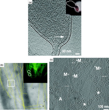
Structures can also be identified through correlated light and electron microscopy (correlated LM/EM). In one strategy, cells with fluorescently tagged targets are applied to an EM grid, imaged by fluorescence light microscopy at room temperature, plunge-frozen, and then imaged again in the electron microscope (Fig. 3a). The location in the tomogram of the tagged target is then found by superposing the LM image on the EM image through appropriate transformations. Of course the LM image is of much lower resolution, so the fluorescent focus spreads beyond the target across larger portions of the cell, but the target lies at the center and repeating the experiment can make the correlation unambiguous. This strategy works well when the molecular target is stationary within a cell, and has been used for instance to localize the bacterial chemoreceptor cluster at the flagellar pole of C. crescentus cells (Briegel et al. Reference Briegel, Ding, Li, Werner, Gitai, Dias, Jensen and Jensen2008). Alternatively, the recent development of cryo-LM stages (Fig. 3b, c) now allows recording of fluorescence images of samples that are already plunge-frozen (Chen et al. Reference Chen, Mcdowall, Dobro, Briegel, Ladinsky, Shi, Tocheva, Beeby, Pilhofer, Ding, Li, Gan, Morris and Jensen2010). This ensures that no molecular movements occur between imaging modalities. Genetically encoded fluorescent tags are better than antibody-targeted tags in all these applications because ‘immunofluorescence’ requires detergent permeabilization (plus lysozyme-treatment for bacteria), which results in grossly altered cell morphology.
Correlated light and electron microscopy. (a) Correlation of mCherry-tagged McpA (inset, red) in a light micrograph of a C. crescentus cell (inset, dotted outline) and of the same cell in an electron cryotomogram. The chemoreceptor array is indicated by an arrow. (b) Low-magnification cryo-EM image showing the positions of individual segmented microtubules (yellow lines), which match those identified by the α-tubulin-GFP fluorescence cryo-light microscopy image of the same cell (upper right panel). (c) Cryotomographic slice of the region boxed in (b) showing microtubules (M), actin filaments (A) and putative ribosomes (asterisks) in a PtK2 cell. Reproduced with permissions from (a) Briegel et al. (Reference Briegel, Ding, Li, Werner, Gitai, Dias, Jensen and Jensen2008) and (b, c) (Schwartz et al. Reference Schwartz, Sarbash, Ataullakhanov, Mcintosh and Nicastro2007).

In organisms that are not yet genetically tractable, proteins can be partially localized in 3D by combining immuno-EM of Tokuyasu cryosections with tomography (Ladinsky & Howell, Reference Ladinsky and Howell2007; Tokuyasu, Reference Tokuyasu1986). While the antibody–gold complex usually only labels the surface of a section, it can provide 3D information if the labeled structure (like a Golgi cisterna; Ladinsky & Howell, Reference Ladinsky and Howell2007) can be tracked deeper into the tomogram.
Where atomic or high-resolution models are available, cryotomograms can be searched for densities of similar size and shape, a procedure that has been named ‘template matching’ (Beck et al. Reference Beck, Malmstrom, Lange, Schmidt, Deutsch and Aebersold2009; Forster, Reference Forster2005; Ortiz et al. Reference Ortiz, Forster, Kurner, Linaroudis and Baumeister2006; Seybert et al. Reference Seybert, Herrmann and Frangakis2006). Ribosomes are particularly recognizable because of their large size (25 nm) and higher-than-average density (from the phosphorus in ribosomal RNA). While potentially very powerful, extension of this type of correlation analysis (‘visual proteomics’; Nickell et al. Reference Nickell, Kofler, Leis and Baumeister2006) to smaller complexes will depend on improvements in image quality and/or the development of better computational searches.
Once a protein or complex is localized and inspected by eye or segmentation, additional information can often be obtained through averaging. Subtomograms that contain the complex of interest are extracted, aligned and averaged, potentially resulting in the elucidation of even high-resolution details. Because the precision of alignment depends on the size of the macromolecular complex and the signal-to-noise ratio of the original tomogram, the most successful applications of this technique to date have been on large dense structures such as the bacterial flagellar motor (Liu et al. Reference Liu, Lin, Botkin, Mccrum, Winkler and Norris2009; Murphy et al. Reference Murphy, Leadbetter and Jensen2006) and ribosomes (Brandt et al. Reference Brandt, Carlson, Hartl, Baumeister and Grunewald2010; Ortiz et al. Reference Ortiz, Brandt, Matias, Sennels, Rappsilber, Scheres, Eibauer, Hartl and Baumeister2010). Periodic and semi-periodic structures are also amenable to subtomographic averaging analysis because the symmetries present can be detected in the power spectra of appropriately oriented slices. In some cases the signal-to-noise ratio can be increased sufficiently to suggest quasi-atomic models (Al-Amoudi et al. Reference Al-Amoudi, Diez, Betts and Frangakis2007; Briegel et al. Reference Briegel, Ding, Li, Werner, Gitai, Dias, Jensen and Jensen2008).
3. Example applications of electron tomography
The first published electron tomography study was of the yeast fatty acid synthase (Hoppe et al. Reference Hoppe, Gassmann, Hunsmann, Schramm and Sturm1974). While the structural insights gained from the resulting tomogram were limited by the chemical fixation and instrumentation, this study was a concrete demonstration that electron tomography of biological specimens was feasible. It took another decade before electron tomography was applied to cellular structures such as Balbiani ring ribonucleoprotein particles (Olins et al. Reference Olins, Olins, Levy, Durfee, Margle, Tinnel and Dover1983; Skoglund et al. Reference Skoglund, Andersson, Strandberg and Daneholt1986), cilia (McEwen et al. Reference Mcewen, Radermacher, Rieder and Frank1986) and chromatin (Belmont et al. Reference Belmont, Sedat and Agard1987). Since then, electron tomography has revealed a wealth of information about cellular ultrastructure, but it is clearly just a beginning. Here we will survey several examples that are by no means comprehensive, but illustrate the kinds and range of questions that can be addressed by tomography.
3.1 Membrane systems involved in vesicular traffic
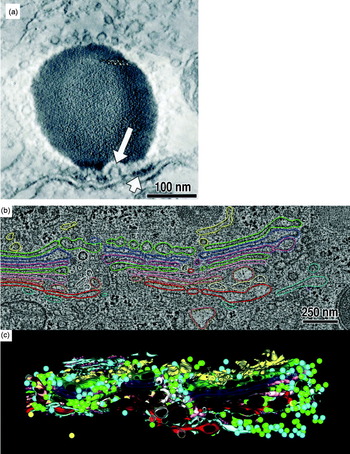
Electron tomography has made – and continues to make – important contributions to our understanding of pleomorphic cellular bodies. Studies of vesicular trafficking are good examples because many vesicles are thinner than the serial thin-sections used for serial-EM reconstructions, and so cannot be well resolved by any other means. An early study of frog saccular hair cells, for example, showed how two classes of vesicles (synaptic and non-synaptic) crowded around the synaptic body in the presynaptic cytoplasm (Lenzi et al. Reference Lenzi, Runyeon, Crum, Ellisman and Roberts1999). Electron tomography revealed rare Ω-shaped profiles in the presynaptic membrane, supporting the idea that membrane recycling was occurring and contributing to the enrichment of vesicles in the synaptic cytoplasm (Fig. 4a). In further experiments in which the cells were subjected to prolonged stimulation, the synaptic body-associated vesicles were depleted on the hemisphere closest to the presynaptic membrane (Lenzi et al. Reference Lenzi, Crum, Ellisman and Roberts2002). This suggested that when a neuron is stimulated, the synaptic vesicles move along the surface of synaptic bodies toward the presynaptic membrane. These studies are also notable as demonstrations of ‘telemicroscopy’ technology that was pioneered at University of California, San Diego (Fan et al. Reference Fan, Mercurio, Young and Ellisman1993).
Electron tomography of vesicular trafficking systems. (a) Tomographic slice of a synapse showing a synaptic body (dense round body~200 nm wide), Ω-shaped presynaptic membrane invagination (long arrow) and presynaptic density (short arrow). (b) Tomographic slice and model (colored) of part of a Golgi body from a normal rat kidney cell. Different colors represent different cisternae. ER-Golgi intermediate compartment – yellow; trans-most cisterna – red. (c) Rendering of the model in 3D. Reproduced with permissions from (a) Lenzi et al. (Reference Lenzi, Runyeon, Crum, Ellisman and Roberts1999) and (b, c) Ladinsky et al. (Reference Ladinsky, Mastronarde, Mcintosh, Howell and Staehelin1999) .

As another example, the Golgi body (also called Golgi apparatus) is depicted in textbooks as a stack of large flattened vesicles called cisternae. In 3D, the Golgi body is a much more complicated network of fenestrated cisternae, tubules, and both coated and uncoated vesicles. Molecular traffic between the cis- and trans-cisternae is bi-directional and must be highly regulated to ensure proper maturation of lipids and proteins. The first 3D models of this remarkable vesicular switchboard were painstakingly constructed using stereoscopic methods (some examples are in Clermont et al. Reference Clermont, Rambourg and Hermo1995), but the visualization of details about the connectivity of cisternal tubules and the distribution of different classes of vesicles, for example, required electron tomography. The Golgi body is so big, however, that a single tomogram cannot capture much of its organization. Instead, ‘montage’ tomograms were acquired from serial sections (Soto et al. Reference Soto, Young, Martone, Deerinck, Lamont, Carragher, Hama and Ellisman1994) and then merged both laterally and ‘vertically’ in silico to reconstruct a 4 μm3 cellular volume (Ladinsky et al. Reference Ladinsky, Mastronarde, Mcintosh, Howell and Staehelin1999). 3D models of this merged serial tomogram illustrate the complexity of the true organization of the Golgi body (Fig. 4b, c) and also led to the discovery of vesicle-filled ‘wells’, which are formed by the aligned fenestrae from a series of cisternae. Subsequent studies showed that in secretory cells, cisterna were often connected by tubules (Marsh et al. Reference Marsh, Volkmann, Mcintosh and Howell2004; Trucco et al. Reference Trucco, Polishchuk, Martella, Di Pentima, Fusella, Di Giandomenico, San Pietro, Beznoussenko, Polishchuk, Baldassarre, Buccione, Geerts, Koster, Burger, Mironov and Luini2004), supporting the idea that the Golgi enzyme retrograde transport mechanism involves more than just vesicular traffic. Ambitious large-scale serial electron-tomography programs are now modeling the Golgi body in medically important systems such as the pancreatic beta cells (Noske et al. Reference Noske, Costin, Morgan and Marsh2008).
3.2 Eukaryotic macromolecular complexes
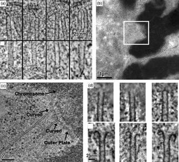
Chromosome segregation is carried out by the conserved machines of the mitotic spindle. Spindles capture sister chromatids and mechanically draw them apart. Historic serial-EM studies classified and counted the microtubules in some key model systems (Ding et al. Reference Ding, Mcdonald and Mcintosh1993; McIntosh et al. Reference Mcintosh, Roos, Neighbors and Mcdonald1985; Winey et al. Reference Winey, Mamay, O'toole, Mastronarde, Giddings, Mcdonald and Mcintosh1995), but did not reveal much about the ends of the microtubules. Detailed in vitro characterization of the dynamic plus end (Chretien et al. Reference Chretien, Fuller and Karsenti1995; Mandelkow et al. Reference Mandelkow, Mandelkow and Milligan1991) and the relatively static minus end (Moritz et al. Reference Moritz, Braunfeld, Guenebaut, Heuser and Agard2000) showed that the structure of microtubule ends might provide clues about their assembly state and function in vivo. Indeed, tomograms of the Saccharomyces cerevisiae spindle pole body revealed that the microtubule minus ends typically have a tapered cap (Fig. 5a), supporting the idea that the gamma-tubulin complex is the conserved nucleation site at the microtubule minus end in vivo (O'Toole et al. Reference O'toole, Winey and Mcintosh1999). These tapered microtubule minus ends were also seen to be general, as they were also found in a subpopulation of spindle microtubules in the higher eukaryote C. elegans (O'Toole et al. Reference O'toole, Mcdonald, Mantler, Mcintosh, Hyman and Muller-Reichert2003). In higher eukaryotes, each chromosome attaches to the plus ends of bundled kinetochore microtubules called K-fibers. Tomograms of K-fiber microtubules showed that the protofilaments were configured into either ‘flared’ or ‘curved’ motifs, indicating that they were either growing or shrinking, respectively. Another tomographic study of individual metazoan K-fibers revealed that 2/3 of the constituent kinetochore microtubules were in the depolymerizing state (Fig. 5b–d). This is surprising because the kinetochore microtubules within a single K-fiber all grow and shrink together, suggesting that the kinetochore itself must regulate the dynamics of microtubule growth and shrinkage (VandenBeldt et al. Reference Vandenbeldt, Barnard, Hergert, Meng, Maiato and Mcewen2006). Ongoing studies seek to determine the mechanism of microtubule-kinetochore attachment (McIntosh et al. Reference Mcintosh, Grishchuk, Morphew, Efremov, Zhudenkov, Volkov, Cheeseman, Desai, Mastronarde and Ataullakhanov2008).
Electron tomography of spindle microtubules. (a) Nuclear (upper panels) and cytoplasmic (lower panels) microtubules from tomograms of S. cerevisiae cells. (b) Low-magnification EM image of a kinetochore (boxed) from a PtK1 cell. Chromosomes are the dark, densely stained objects. (c) Tomographic slice of the region boxed in (b), showing the curved morphologies of two kinetochore microtubule plus ends. (d) Gallery showing that kinetochore plus ends exhibit both blunt/straight and curved (ram's horn) morphologies. Reproduced with permissions from (a) O'Toole et al. (Reference O'toole, Winey and Mcintosh1999) and (b–d) Vandenbeldt et al. (Reference Vandenbeldt, Barnard, Hergert, Meng, Maiato and Mcewen2006) .

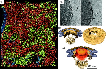
In 2002, a seminal cryotomographic study was published on the slime mold Dictyostelium discoideum (Medalia et al. Reference Medalia, Weber, Frangakis, Nicastro, Gerisch and Baumeister2002). Cells were grown on EM grids, plunge-frozen, and then imaged. Since Dictyostelium cell bodies are more than 1 μm thick, only their peripheries were accessible. The resulting cryotomograms revealed the cytoplasm to be densely packed with actin filaments and large macromolecular complexes including ribosomes and 26S proteasomes (Fig. 6a). Contemporary studies on the thin leading edges of cells include lamellipodia (Urban et al. Reference Urban, Jacob, Nemethova, Resch and Small2010) and focal adhesions (Patla et al. Reference Patla, Volberg, Elad, Hirschfeld-Warneken, Grashoff, Fassler, Spatz, Geiger and Medalia2010), which are both rich in actin and actin-binding proteins. The densely packed macromolecules in these cryotomograms are reminiscent of the beautiful watercolors by David Goodsell (Goodsell, Reference Goodsell2005), and highlight how crowded cells can be (Minton, Reference Minton2006).
Electron cryotomography of eukaryotic cells. (a) Surface rendering showing actin (red), putative ribosomes (green) and membranes (blue) at the periphery of a frozen-hydrated Dictyostelium discoideum cell. (b) Cryotomographic slices of an intact Dictyostelium nucleus showing top (left) and side (right) views of the NPC (arrows). Patches of ribosome-studded rough ER are indicated by arrowheads. (c) Subtomographic average of the NPC. (d) Probability density (orange) of gold-labeled classical import cargoes. Reproduced with permissions from (a) Medalia et al. (Reference Medalia, Weber, Frangakis, Nicastro, Gerisch and Baumeister2002), (b) Beck et al. (Reference Beck, Forster, Ecke, Plitzko, Melchior, Gerisch, Baumeister and Medalia2004) and (c, d) Beck et al. (Reference Beck, Lucic, Forster, Baumeister and Medalia2007) .

Isolated, frozen-hydrated ‘transport-competent’ Dictyostelium nuclei with functional NPCs have also been imaged (Beck et al. Reference Beck, Forster, Ecke, Plitzko, Melchior, Gerisch, Baumeister and Medalia2004). Slices through these isolated nuclei revealed nuclear pores embedded in the nuclear envelope, which was further decorated on the outer membrane by ribosomes (Fig. 6b). Subvolumes containing these NPCs were extracted from the tomograms, aligned, and then averaged to generate a higher-resolution ‘subtomographic average’ of the active NPC (Fig. 6c). An elegant follow-up study showed the positions of gold-labeled test cargos, which could be mapped as a probability density cloud within the central channel of the NPC (Beck et al. Reference Beck, Lucic, Forster, Baumeister and Medalia2007). The good match between the shape of the cargo density and the previously described central plug/transporter density supported the idea that the central plug/transporter is the cargo itself (Fig. 6d). Interestingly, the NPC appears to be somewhat distorted in situ, but adopts strong 8-fold rotational symmetry when purified (Yang et al. Reference Yang, Rout and Akey1998). It remains to be seen if the deviation from symmetry in situ is a result of active transport, i.e., structural distortion to promote passage of the cargo molecule. These studies illustrate how tomography can be used to visualize different conformations of objects within their cellular context.
3.3 Tomography of tissues
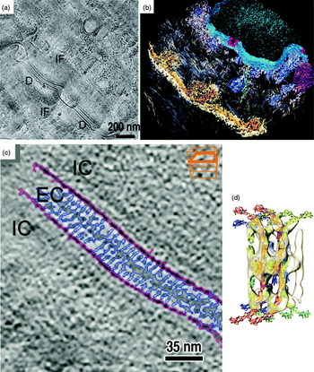
To understand the 3D ultrastructure of thicker frozen-hydrated specimens, a few groups have started to use electron cryotomography to image cryosections (Bouchet-Marquis et al. Reference Bouchet-Marquis, Zuber, Glynn, Eltsov, Grabenbauer, Goldie, Thomas, Frangakis, Dubochet and Chretien2007; Hsieh et al. Reference Hsieh, Marko, Frank and Mannella2002). In a recent study of desmosomes (the proteinaceous intercellular junctions that adhere cells together in many tissues) for example, a human skin biopsy sample was high-pressure-frozen, cryosectioned, and imaged by electron cryotomography (Al-Amoudi et al. Reference Al-Amoudi, Diez, Betts and Frangakis2007) (Fig. 7). The cryotomograms revealed that the cadherin molecules were densely and uniformly packed, a result that differed from that of an earlier study of high-pressure-frozen/freeze-substituted skin, in which some cadherins formed discrete clusters (He et al. Reference He, Cowin and Stokes2003). Subtomographic averaging of the cryotomographic densities produced an ~3.4 nm resolution average, which was interpreted with the X-ray crystal structure of a ‘classical’ cadherin (Boggon et al. Reference Boggon, Murray, Chappuis-Flament, Wong, Gumbiner and Shapiro2002). The quasi-atomic model of the desmosomes showed that the cadherins were highly flexible, but interacted predominantly at the midline between cells. This work represents an exciting starting point to the molecular characterization of diseases associated with malfunctioning desmosomes.
Electron cryotomography of vitreous tissue sections. (a) Cryo-EM image of a cryosectioned human skin biopsy showing desmosomes (D) and filament networks (IF). (b) Isosurface rendering of a cryotomogram from another region of skin showing desmosomes (gold/brown), the nucleus (blue), nuclear pores (red) and a putative microtubule (green). (c) Cryotomographic slice of a desmosome showing extracellular (EC) and intracellular (IC) spaces. (d) Subtomographic average of C-cadherin molecules (white isosurfaces) with crystal structures docked. Reproduced with permission from Al-Amoudi et al. (Reference Al-Amoudi, Diez, Betts and Frangakis2007) .

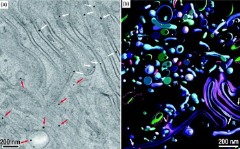
An ongoing challenge in electron microscopy is the localization and identification of proteins and protein complexes in 3D images of cells. A significant advance was made in this direction by He et al., who were able to follow immunoglobulin G (IgG) transcytosis through jejunal cells in the small intestine (He et al. Reference He, Ladinsky, Huey-Tubman, Jensen, Mcintosh and Bjorkman2008). In this study, neonatal rats were fed a ‘milk’ solution containing gold-conjugated IgG. After the IgGs were endocytosed, the rats were killed and parts of the small intestines near the jejunum were excised and immediately high-pressure-frozen. To enhance the contrast of the IgG-coupled gold tag, the intestinal tissue was treated with silver at low temperature using the same solvents needed for the subsequent FS step (He et al. Reference He, Kivork, Machinani, Morphew, Gail, Tesar, Tiangco, Mcintosh and Bjorkman2007; Morphew et al. Reference Morphew, He, Bjorkman and Mcintosh2008). The tissue was then subjected to FS, plastic embedding and microtomy. Tomograms from the resulting plastic sections clearly showed tags in a diversity of vesicles and between cells in the lateral intercellular space (Fig. 8). Further development of this experimental system may yield a complete IgG molecular-trafficking map from the apical to the basolateral side of an entire cell.
Transcytosis followed in tissues. (a) Tomographic slice of the lateral intercellular space (LIS) between two neonatal rat jejunal cells. Gold-labeled Fc (Au-Fc) molecules can be found in both the LIS (red arrows) and irregular vesicles (white arrows). (b) 3D segmentation of the region in (a) showing membranes and vesicles in green and blue, and Au-Fc in gold. Reproduced with permission from He et al. (Reference He, Ladinsky, Huey-Tubman, Jensen, Mcintosh and Bjorkman2008) .

3.4 Bacterial ultrastructure
Filaments were so rarely seen in traditional thin-section EM images of bacteria that their absence was long thought to be one of the distinguishing characteristics of ‘prokaryotes’. The advent of higher-resolution fluorescence light microscopes and GFP-tagging methods then revolutionized bacterial cell biology by suggesting that numerous bacterial proteins form helices, rings and other filaments (Gitai, Reference Gitai2005). Electron cryotomography has proven essential in clarifying, adding to, and in some cases refuting these claims.
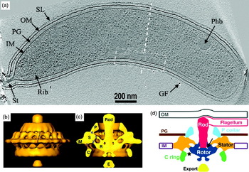
Cytoskeletal filaments were first directly visualized by electron cryotomography in the thin spiral-shaped bacterium Spiroplasma melliferum (Kurner et al. Reference Kurner, Frangakis and Baumeister2005). In the classic model species C. crescentus, multiple classes of filaments including ‘cytoplasmic’, ‘ring-like’, ‘polar’ and ‘inner curvature’ were then discovered (Briegel et al. Reference Briegel, Dias, Li, Jensen, Frangakis and Jensen2006). The latter class of filaments (Fig. 9a) were later shown by correlated LM-electron cryotomography experiments to be polymers of CTP synthase that negatively regulated cell curvature (Ingerson-Mahar et al. Reference Ingerson-Mahar, Briegel, Werner, Jensen and Gitai2010). More filaments were discovered by cryotomography in the Gram-negative magnetotactic bacterium Magnetospirillum magneticum, this time flanking linear arrays of magnetosomes (a bacterial ‘organelle’ that contains a magnetite crystal and aligns the cell to the geomagnetic field) (Komeili et al. Reference Komeili, Li, Newman and Jensen2006; Scheffel et al. Reference Scheffel, Gruska, Faivre, Linaroudis, Plitzko and Schuler2006). These filaments were identified as the actin-like protein MamK. The cryotomograms also delivered an unexpected surprise: the magnetosomes were not true organelles in which the membranes formed closed vesicles, but were instead simply invaginations of the inner membrane. A second bacterial actin homolog, ParM, was seen forming bundles of filaments in situ, clarifying the number and arrangement of filaments in these plasmid-segregating machines (Salje et al. Reference Salje, Zuber and Lowe2009). Filaments of the tubulin-like FtsZ protein were visualized in dividing C. crescentus cells (Li et al. Reference Li, Trimble, Brun and Jensen2007). Instead of complete rings as expected from fluorescence light microscopy, FtsZ was shown to form short arc-like fragments adjacent to the inner membrane of the constriction site. The filaments adopted both straight and curved conformations, which supported an ‘iterative pinching’ model for cell constriction (Erickson, Reference Erickson1997).
Insights into bacterial ultrastructure. (a) Cryotomographic slice of a Caulobacter crescentus cell showing the inner curvature filaments (white dashed box). Other features include the S-layer (SL), outer membrane (OM), peptidoglycan layer (PG), inner membrane (IM), stalk (St), putative ribosomes (Rib), putative poly-β-hydroxybutyrate granule (Phb) and gold fiducial (GF). (b) Isosurface rendering of a Treponema primitia flagellar motor subtomographic average. (c) Cutaway of (b), with components labeled: peptidoglycan-binding collar (P), stator (S), rotor (R), cytoplasmic ring (C), putative export structure (E) and inner membrane (IM). (d) Cartoon of the motor's organization based on the cryotomography data. Reproduced with permissions from Briegel et al. (Reference Briegel, Dias, Li, Jensen, Frangakis and Jensen2006) and Murphy et al. (Reference Murphy, Leadbetter and Jensen2006) .

It is noteworthy that magnetosomes and dividing bacterial cells had been thoroughly studied using traditional EM, but the MamK and FtsZ filaments were never detected, probably because the chemical fixation and dehydration caused them to depolymerize (Pilhofer et al. Reference Pilhofer, Ladinsky, Mcdowall and Jensen2010). In contrast, certain filaments that were thought to exist based on fluorescence microscopy have not been detected in cryotomograms. The actin homolog MreB, for instance, was reported to form long helices surrounding rod-shaped cells just inside their cytoplasmic membranes (Chiu et al. Reference Chiu, Chen and Wong2008; Figge et al. Reference Figge, Divakaruni and Gober2004; Jones et al. Reference Jones, Carballido-Lopez and Errington2001; Shih et al. Reference Shih, Le and Rothfield2003; Srivastava et al. Reference Srivastava, Demarre, Karpova, Mcnally and Chattoraj2007). Puzzlingly, no such helices were ever seen in cryotomograms (Swulius et al. Reference Swulius, Chen, Jane Ding, Li, Briegel, Pilhofer, Tocheva, Lybarger, Johnson, Sandkvist and Jensen2011). New fluorescence images are now showing the helical patterns seen previously by light microscopy were apparently just artifacts (Dominguez-Escobar et al. Reference Dominguez-Escobar, Chastanet, Crevenna, Fromion, Wedlich-Soldner and Carballido-Lopez2011; Garner et al. Reference Garner, Bernard, Wang, Zhuang, Rudner and Mitchison2011).
Electron cryotomography has also been instrumental in the study of megadalton-sized bacterial molecular machines in their native context. This is especially true for the bacterial flagellar motor, which cannot be purified intact because it loses the torque-generating ‘stator’ component (Tang et al. Reference Tang, Braun and Blair1996; Thomas et al. Reference Thomas, Morgan and Derosier2001). Intact flagellar motors were first visualized in cryotomograms of the spirochaete Treponema primitia, a bacterium with periplasmic flagella (Murphy et al. Reference Murphy, Leadbetter and Jensen2006). The motor was then reconstructed to ~7 nm resolution by subtomographic averaging and the imposition of 16-fold rotational symmetry (Fig. 9b–d). In contrast to the flagellar motors of other bacteria, the Treponema motor is unusually wide, suggesting how it might generate the higher levels of torque needed to rotate the flagellum within the periplasm (Murphy et al. Reference Murphy, Matson, Leadbetter, Berg and Jensen2008). Indeed, flagellar motors from the Borrelia spirochaetes shared a similar architecture (Kudryashev et al. Reference Kudryashev, Cyrklaff, Wallich, Baumeister and Frischknecht2010; Liu et al. Reference Liu, Lin, Botkin, Mccrum, Winkler and Norris2009). A recent cryotomographic comparison of 11 different motors has highlighted how this amazing molecular machine has evolved to meet the needs of different species (Chen et al. Reference Chen, Beeby, Murphy, Leadbetter, Hendrixson, Briegel, Li, Shi, Tocheva, Muller, Dobro and Jensen2011).
Subtomographic averaging has also furthered our understanding of bacterial chemotaxis. Bacteria sense molecules in their environment and regulate the direction of their swimming using an array of chemoreceptors embedded in the inner membrane. These arrays are exquisitely sensitive, and can dynamically adjust their response to a staggering five orders-of-magnitude range of attractant concentrations (Alon et al. Reference Alon, Surette, Barkai and Leibler1999). While X-ray crystallography and NMR spectroscopy have delivered atomic models of various components of this signaling system, cryotomography showed that the receptors are universally organized in vivo in hexagonal arrays of trimers-of-receptor-dimers (Briegel et al. Reference Briegel, Ding, Li, Werner, Gitai, Dias, Jensen and Jensen2008, Reference Briegel, Ortega, Tocheva, Wuichet, Li, Chen, Muller, Iancu, Murphy, Dobro, Zhulin and Jensen2009; Khursigara et al. Reference Khursigara, Wu and Subramaniam2008a, Reference Khursigara, Wu, Zhang, Lefman and Subramaniamb), providing a basis for mechanistic models of the cooperativity.
3.5 Virus-cell interactions
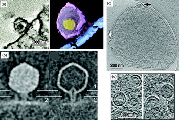
While cryo-EM single particle analysis has been used to study symmetric viral capsids (Liu et al. Reference Liu, Jin, Koh, Atanasov, Schein, Wu and Zhou2010; Wolf et al. Reference Wolf, Garcea, Grigorieff and Harrison2010), tomography has been needed to understand asymmetric viral particles like Herpesvirus (Grunewald et al. Reference Grunewald, Desai, Winkler, Heymann, Belnap, Baumeister and Steven2003), HIV (Benjamin et al. Reference Benjamin, Ganser-Pornillos, Tivol, Sundquist and Jensen2005; Briggs et al. Reference Briggs, Grunewald, Glass, Forster, Krausslich and Fuller2006; Wright et al. Reference Wright, Schooler, Ding, Kieffer, Fillmore, Sundquist and Jensen2007), influenza (Harris et al. Reference Harris, Cardone, Winkler, Heymann, Brecher, White and Steven2006) and bunyaviruses (Overby et al. Reference Overby, Pettersson, Grunewald and Huiskonen2008). In addition, tomography has proven vital to visualize the interactions of viruses with their cellular hosts, both during infection and assembly/egress. The following three recent tomographic studies, taken from the eukaryotic, bacterial and archael domains of life, respectively, are good examples.
In a study of Simian immunodeficiency virus (SIV) and HIV-1 entry, viruses were incubated briefly with cell lines expressing the appropriate receptors and co-receptors (Sougrat et al. Reference Sougrat, Bartesaghi, Lifson, Bennett, Bess, Zabransky and Subramaniam2007). The cell/virus infection mixture was then fixed, plastic-embedded, sectioned and imaged. Tomograms showed that both SIV and HIV engaged their target cells with an ‘entry claw’ (Fig. 10a) that apparently concentrates virus glycoprotein spikes and possibly host receptors in a small patch of 5–7 large densities. Surprisingly, glycoprotein spikes were largely absent from the non-interacting hemisphere of the virion. Further work using this retrovirus infection system should help resolve longstanding questions about what conformational changes drive cell–virus membrane fusion (White et al. Reference White, Bartesaghi, Borgnia, Meyerson, De La Cruz, Bess, Nandwani, Hoxie, Lifson, Milne and Subramaniam2010).
Virus–cell interactions. (a) Tomographic slice (left) and surface rendering (right) of HIV-1 bound to a T-cell. Structures are colored as: viral membrane (purple), core (yellow), cell membrane (blue) and ‘entry claw’ contacts (red). (b) Central slices through the subtomographic averages of full (left) and emptied (right) ∊15 bacteriophages bound to Salmonella hosts. (c) Cryotomographic slice of a Sulfolobus solfataricus cell, infected with Sulfolobus turreted icosahedral virus (STIV). Virus-induced pyramids appeared with electron-dense bodies (black arrow) or without supermolecular complexes (white arrow). (d) Cryotomographic slices of partially assembled (p), empty (e) and filled (f) STIV. Reproduced with permissions from Sougrat et al. (Reference Sougrat, Bartesaghi, Lifson, Bennett, Bess, Zabransky and Subramaniam2007), Fu et al. (Reference Fu, Wang, Gan, Lanman, Khayat, Young, Jensen, Doerschuk and Johnson2010) and Chang et al. (Reference Chang, Schmid, Haase-Pettingell, Weigele, King and Chiu2010) .

A different study investigated the conformational changes that dsDNA bacteriophage undergo when infecting their bacterial hosts (Chang et al. Reference Chang, Schmid, Haase-Pettingell, Weigele, King and Chiu2010). Phage ∊15 were mixed with Salmonella and sites where phage had docked onto the host cell were imaged with electron cryotomography (Fig. 10b). Some phages exhibited DNA-filled heads whereas other phages had already injected their genomes and were therefore empty. A comparison of the full and empty phage showed that the tail must undergo major conformational changes to inject the viral genome. The tail hub extends a tube that spans the entire periplasm, presumably protecting the viral DNA from degradation. In the emptied phage, the tail's interior channel appears tapered, possibly to seal up the injection site.
Archael viruses can drastically alter the structure of their hosts, as illustrated by a 3D study of the last stages of infection (Fu et al. Reference Fu, Wang, Gan, Lanman, Khayat, Young, Jensen, Doerschuk and Johnson2010). Here, Sulfolobus cells were infected with the Sulfolobus turreted icosahedral virus, a dsDNA virus of the Adeno-PRD1 lineage that has an internal lipid membrane layer (Khayat et al. Reference Khayat, Tang, Larson, Lawrence, Young and Johnson2005). After the infection had progressed for many hours, Sulfolobus cells were plunge-frozen and imaged by electron cryotomography. The cryotomograms showed new details about the pyramid structures that protrude from the cell surface (Brumfield et al. Reference Brumfield, Ortmann, Ruigrok, Suci, Douglas and Young2009) (Fig. 10c). In the cytoplasm, some partially assembled viruses were discovered, revealing a partial capsid protein shell and a partial lipid layer (Fig. 10d). This unexpected finding suggests that in Sulfolobus turreted icosahedral virus (STIV) and related viruses, the capsid and lipid membrane co-assemble in the cytoplasm. This de novo assembly of viral membrane is especially intriguing because uninfected Sulfolobus cells apparently do not assemble cytoplasmic vesicles or organelles. Much of the early (initial infection) and terminal (lysis) stages of the STIV lifecycle remain to be characterized.
4. Future developments
Given electron tomography's ability to reveal the ultrastructure of cells and other unique biological objects in 3D to macromolecular resolution, it is likely to have a long and powerful impact on cell biology. The technique is still young, however, and so there are many opportunities for improvement.
4.1 Better specimens
The quality of any image is limited by the quality of the specimen. Unfortunately, since only slender bacterial and archaeal cells and the thin edges of some eukaryotic cells are thin enough to image directly (see above), the majority of eukaryotic cells and many bacterial and archaeal cells must be sectioned. While this is straightforward to do after plastic-embedding, efforts are underway to develop techniques to allow the interiors of these cells to be imaged in the more life-like, frozen-hydrated state. While thin vitreous sections can be produced by cryoultramicrotomy (Al-Amoudi et al. Reference Al-Amoudi, Chang, Leforestier, Mcdowall, Salamin, Norlen, Richter, Blanc, Studer and Dubochet2004), this technique generates low yields of good specimens. In a recent study that highlights this technology's promise, however, hundreds of tilt series were recorded from cryosection ribbons of the picoplankton Ostreococcus tauri, a tiny eukaryote just ~0.5–1 μm thick (Gan et al. Reference Gan, Ladinsky and Jensen2011; Henderson et al. Reference Henderson, Gan and Jensen2007). Individual microtubule protofilaments could be resolved in the vitreous ice deep within the nucleus, and revealed the surprising result that O. tauri segregates its genome with fewer microtubules than chromosomes. Technologies such as micromanipulator-assisted handling of the elongating cryosection (Ladinsky et al. Reference Ladinsky, Pierson and Mcintosh2006), electrostatic charging of the cryosection to make it adhere to the grid without the use of mechanical stamping (Pierson et al. Reference Pierson, Fernandez, Bos, Amini, Gnaegi, Vos, Bel, Adolfsen, Carrascosa and Peters2010), and the solubilization of quantum dots or gold colloids in cryogenic organic solvents for deposition onto cryosections (Gruska et al. Reference Gruska, Medalia, Baumeister and Leis2008; Masich et al. Reference Masich, Ostberg, Norlen, Shupliakov and Daneholt2006) may improve the yield in the future.
As mentioned above, cryosections today also suffer from compression along the cutting direction and crevasses and knife marks on the two faces (Dubochet et al. Reference Dubochet, Zuber, Eltsov, Bouchet-Marquis, Al-Amoudi and Livolant2007). Crevasses can be somewhat reduced when cryosections are cut just 20 nm thick (Zhang et al. Reference Zhang, Bos, Heymann, Gnaegi, Kessel, Peters and Subramaniam2004), but this severely reduces the cellular volume sampled in each tomogram. Recently, the cryo focused-ion-beam (FIB) milling method was developed as a way to produce cryosections with minimal ‘cutting’ artifacts (Hayles et al. Reference Hayles, Matthijs De Winter, Schneijdenberg, Meeldijk, Luecken, Persoon, De Water, De Jong, Humbel and Verkleij2010; Marko et al. Reference Marko, Hsieh, Schalek, Frank and Mannella2007; Rigort et al. Reference Rigort, Bauerlein, Leis, Gruska, Hoffmann, Laugks, Bohm, Eibauer, Gnaegi, Baumeister and Plitzko2010). Here, a beam of ions (typically Gallium) is used to thin a pellet of high-pressure-frozen cells. Because there is no mechanical cutting, there are fewer surface artifacts. FIB milling can only generate one cryosection per experiment, however, prohibiting serial sectioning. As with traditional plastic-embedding, and then FS, advances such as plunge-freezing and cryosectioning have revealed new details and caused some earlier images to be reinterpreted. Thus, while we have certainly been moving towards more native specimens, history reminds us to remain cautious about our conclusions no matter how advanced our methods are.
4.2 Better images
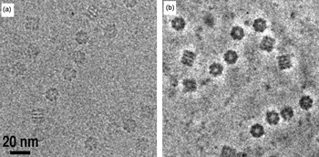
Cryo-EM images have low contrast in part because the phase CTF has a sinusoidal shape and starts with zero contrast transfer at zero spatial frequency. There is a small amount of cosine-like amplitude contrast, but its contribution from light elements like carbon, nitrogen and oxygen is small. Low-resolution phase contrast can be increased substantially by using a phase plate (Nagayama & Danev, Reference Nagayama and Danev2009). As in phase-contrast light microscopy, the scattered beam is made to undergo a phase shift relative to the unscattered beam either by passing through a thin amorphous carbon film (Danev & Nagayama, Reference Danev and Nagayama2008) or an electric field (Cambie et al. Reference Cambie, Downing, Typke, Glaeser and Jin2007; Majorovits et al. Reference Majorovits, Barton, Schultheiss, Perez-Willard, Gerthsen and Schroder2007). The unscattered and scattered electrons then recombine at the image plane to form a higher contrast image generated through a cosine-like CTF. Images from the first generation of phase plates show impressive increases in low frequency contrast (Fig. 11), but it remains to be seen whether any new high-resolution details are also recoverable. If a spherical-aberration corrector and a phase plate were combined, the oscillations of the CTF and the challenges of the defocus gradient could be nearly eliminated in the resolution range of interest in electron tomography (Danev et al. Reference Danev, Glaeser and Nagayama2009).
Zernike phase-contrast. Cryo-EM of GroEL with (a) defocus phase contrast and (b) Zernike phase contrast generated by a thin amorphous-carbon phase plate. Reproduced with permission from Danev & Nagayama (Reference Danev and Nagayama2008) .

Current phosphor-CCD detectors suffer from large point spread functions and high noise from the electron–photon conversion process. A number of groups have now made progress designing and fabricating ‘direct’ detectors, semiconductor devices that generate signal from the impact of the high-energy imaging electrons themselves (Deptuch et al. Reference Deptuch, Besson, Rehak, Szelezniak, Wall, Winter and Zhu2007; McMullan et al. Reference Mcmullan, Cattermole, Chen, Henderson, Llopart, Summerfield, Tlustos and Faruqi2007; Milazzo et al. Reference Milazzo, Leblanc, Duttweiler, Jin, Bouwer, Peltier, Ellisman, Bieser, Matis, Wieman, Denes, Kleinfelder and Xuong2005). Direct detectors should also read-out quickly enough to discriminate individual electron hits, allowing each imaging electron to be counted with equal weight. These two factors will dramatically improve the modulation transfer function (McMullan et al. Reference Mcmullan, Clark, Turchetta and Faruqi2009), resulting in a nearly perfect detector.
4.3 Better analyses
The most time-consuming step in electron tomography today is the analysis of the tomograms. More powerful and automatic methods to calculate, refine, denoise, segment and search tomograms are needed. To identify proteins of interest, high contrast genetically encodable tags are being developed. The metal-binding protein metallothionein appears in vitro to be an attractive candidate (Mercogliano & DeRosier, Reference Mercogliano and Derosier2007), though it remains to be seen if metallothionein-gold tags can be localized in 3D electron cryotomograms of cells and how broadly this tag can be applied (Diestra et al. Reference Diestra, Fontana, Guichard, Marco and Risco2009). Ferritin-based tags may also be used to localize proteins, as recently demonstrated in cryotomograms of bacterial cells (Wang et al. Reference Wang, Mercogliano and Lowe2011). Another promising tagging strategy for plastic-embedded samples is the ReAsh–diaminobenzadine (ReAsh–DAB) system, which allows co-localization of ReAsh in fluorescence images and DAB-nucleated osmium haloes in EM images (Gaietta et al. Reference Gaietta, Deerinck, Adams, Bouwer, Tour, Laird, Sosinsky, Tsien and Ellisman2002). It remains to be seen, however, how precisely the DAB-osmium halo could localize a smaller object in 3D in a tomogram.
While the real power of tomography is its ability to produce a 3D image of a single unique object, when there are multiple copies of a particular structure in a cell or a group of cells, additional information can be gained by classification and averaging. New and better tools (both software and hardware) for this are needed. As an example, the maximum-likelihood method (Sigworth, Reference Sigworth1998) promises to improve the averaging of particles from cellular environments, where many will exhibit conformational heterogeneity and differences in assembly state. Classification and alignment of subtomograms are done simultaneously and the missing wedge is treated as unobserved data (Scheres et al. Reference Scheres, Melero, Valle and Carazo2009). The reconstructions are generated in iterations in which a weighted average of all possible alignments and class assignments contributes to the reconstruction in each cycle. Since the maximum-likelihood method is robust to missing data, noisy data, and conformational heterogeneity, it can produce model-bias-free subtomographic reconstructions, but it is computationally demanding (Fu et al. Reference Fu, Wang, Gan, Lanman, Khayat, Young, Jensen, Doerschuk and Johnson2010; Ortiz et al. Reference Ortiz, Brandt, Matias, Sennels, Rappsilber, Scheres, Eibauer, Hartl and Baumeister2010).
5. Conclusion
Electron tomography has begun to deliver 3D images of cells with sufficient resolution to visualize the structure of large macromolecular complexes and their arrangement in situ. Such images are vital, since in many cases structures of interest only assemble or only exhibit functional conformations in their cellular environment. Usually, tomographic imaging leads directly to mechanistic hypotheses. Thus while the contributions of electron tomography to eukaryotic, bacterial and archael cell biology have already been substantial (see examples above), we believe it is just the beginning. Improved methods for serial cryosectioning and labeling will dramatically expand the utility of electron tomography in coming years. EMs capable of tomography are still rare, expensive and frequently out of service, but many institutions are now investing in these instruments and new research groups are rapidly sprouting up around the world with the expertise to exploit them. The development of direct detectors, phase plates and aberration correctors will dramatically improve the information content of future tilt series, and both the software tools and the raw computational power needed to extract structural details from the tomograms are increasing. Electron tomograms will increasingly be the ‘place’ where sequencing ‘parts lists’, atomic models, biochemical measurements and single-molecule biophysical data meet to reveal mechanism.
6. Acknowledgements
We thank Morgan Beeby, Ariane Briegel, Mark Ladinsky, Alasdair McDowall and Martin Pilhofer for comments and Karin Mallard for help with figures and editing. We apologize to all our colleagues whose work we could not highlight for space constraints. This work was supported in part by NIH grants GM066521 and GM094800B to G. J. J.