

Introduction
The distribution of surnames is not random across time and space (Darlu et al., Reference Darlu, Bloothooft, Boattini, Brouwer, Brouwer and Brunet2012). Naming practices reflect social norms and ethno-cultural customs. These practices have been developed and transmitted over generations and are often maintained after migrations (Mateos et al., Reference Mateos, Longley and O’Sullivan2011). Naming is thus the product of cultural, linguistic and legislative processes that have enabled its normalization and systematic transmission (Cheshire, Reference Cheshire2014). As a source of social, cultural and historical information, the study of surnames makes it possible to trace the history of populations over the centuries. The accessibility of surnames at various times and their reliability as a historical–demographic source (Boattini et al., Reference Boattini, Calboli, Villegas, Gueresi, Franceschi and Paoli2006) have made them very interesting for the reconstruction of human genetic structures. The analogy between genes and surnames, due to their patrilineal transmission since the Middle Ages in most European countries, has allowed the emergence of numerous methodologies (Mourrieras et al., Reference Mourrieras, Darlu, Hochez and Hazout1995).
As early as 1965, Crow and Mange developed the theory of isonymy in order to estimate the relationship between consanguinity and family names (Crow & Mange, Reference Crow and Mange1965). Originally, their calculations were based on marriage registers because they believed that isonymous unions (same name) would often correspond to a marriage between first cousins (Crow & Mange, Reference Crow and Mange1965). Since then, the use of isonymy theory has been extended to larger databases and allows for the estimation of diversity or isolation of human groups.
Generally, studies analysing the structure of the French population in the 20th century using surnames use the ‘surname file’ designed in the 1970s by INSEE (Mourrieras et al., Reference Mourrieras, Darlu, Hochez and Hazout1995; Darlu et al., Reference Darlu, Degioanni and Ruffie1997; Vernay, Reference Vernay2001; Darlu & Oyharçabal, Reference Darlu and Oyharçabal2006; Gibert et al., Reference Gibert, Roumieu, Telmon, Sangoi and Sevin2012). This file provides the names of natives, geographically referenced at the commune level, from the period 1891 to 1990. The studies concerning the 21st century are based on the telephone directory (Scapoli et al., Reference Scapoli, Goebl, Sobota, Mamolini, Rodriguez-Larralde and Barrai2005). These studies have shown that south-eastern France differed from the rest of the country in the 20th century because the Massif Central seemed to act as a migration barrier (Mourrieras et al., Reference Mourrieras, Darlu, Hochez and Hazout1995). For the 21st century, Scapoli et al. (Reference Scapoli, Goebl, Sobota, Mamolini, Rodriguez-Larralde and Barrai2005) showed that the French population is structured according to different cultural and linguistic phenomena.
This study looked at different levels of administrative division, among which the departmental analysis of France showed the isolation of the Alpes-Maritimes department (located in the south-east) from the French territory. The aim of the study, therefore, was to analyse the distribution of surnames of an earlier period, the 19th century, in order to grasp the micro-evolution and the particularities of the Sud-Provence-Alpes-Côte d’Azur region, and then to identify the isonymic structures of the population studied in order to evaluate the impact of geographical remoteness and historical, migratory, cultural and linguistic phenomena on these structures. There is a fairly extensive bibliography on the migration history of the southern region. These sources emphasize the importance of the rural exodus of the 20th century, which began in the middle of the 19th century and demographically strengthened the cities (Marseille, Nice, Toulon, etc.). At the same time, there are reflections on the extent of migratory movements in the old French village society (Dupâquier, Reference Dupâquier2002). This study contributes to the debate on rural society and migration by providing elements of a response through the use of an original and never-before-exploited database. Furthermore, the results of this new analysis, coupled with the analogy between isonymic and genetic structures, suggest several types of applications in the field of public health, which are developed in terms of perspectives.
Methods
Study area and population
The Sud-Provence-Alpes-Côte d’Azur region, located in the south-east of France, is one of the thirteen French regions and covers 31,400 km2. To the west, the Rhône River forms its regional boundary with Occitania, while to the north it borders on the Auvergne-Rhône-Alpes region. The Italian regions of Liguria and Piedmont border the region to the east, and to the south it is bordered by the Mediterranean Sea. Both the borders and the name of the Sud-Provence-Alpes-Côte d’Azur region have varied over the centuries. In 1972, the Provence-Alpes-Côte d’Azur region was administratively created by the French state and designated by the acronym PACA, but since 2018 it has been called the Sud-Provence-Alpes-Côte d’Azur region by the regional council. This territory includes six departments, three of which are coastal: Bouches-du-Rhône, Alpes-Maritimes and Var; the other three are located inland: Vaucluse, Alpes-de-Haute-Provence and Hautes-Alpes. These departments originate from the former provinces of Provence, the Dauphiné for the Hautes-Alpes, the Comtat Venaissin for the Vaucluse and the Comté de Nice for the Alpes-Maritimes. The southern region offers a wide variety of contrasting landscapes (plains, hills, mountains and coastline), whose cohesion is ensured by the routes traced by the Durance and the Rhône (Bouvier, Reference Bouvier1979; Temime, Reference Temime1997).
According to the National Institute of Statistics and Economic Studies (INSEE), the region had more than 5 million inhabitants in 2018 (Michaïlesco & Mora, Reference Michaïlesco and Mora2020), whereas in the 1851 census its population did not exceed 1.5 million (Le Mée, Reference Le Mée1999). The demographic growth of the region has therefore been spectacular due to socioeconomic changes and migration (Gastaut, Reference Gastaut2009). It is now a highly urbanized region; 90% of its inhabitants are city dwellers, whereas at the beginning of the 19th century, 60% of its population lived from agriculture (Gastaut, Reference Gastaut2009). The distribution of the population is now very unbalanced. The technical, industrial and tourist progress of the 20th century, located on the Rhône axis and on the coast (Marseille, Nice, Toulon), has attracted migrants to these new centres of attraction, which today accommodate three-quarters of the region’s inhabitants (Gastaut, Reference Gastaut2009). As a result, the interior of the peasant region, which traditionally subsisted on olive trees, vines and wheat, was economically weakened and depopulated during the rural exodus (Temime, Reference Temime1997).
Data
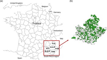
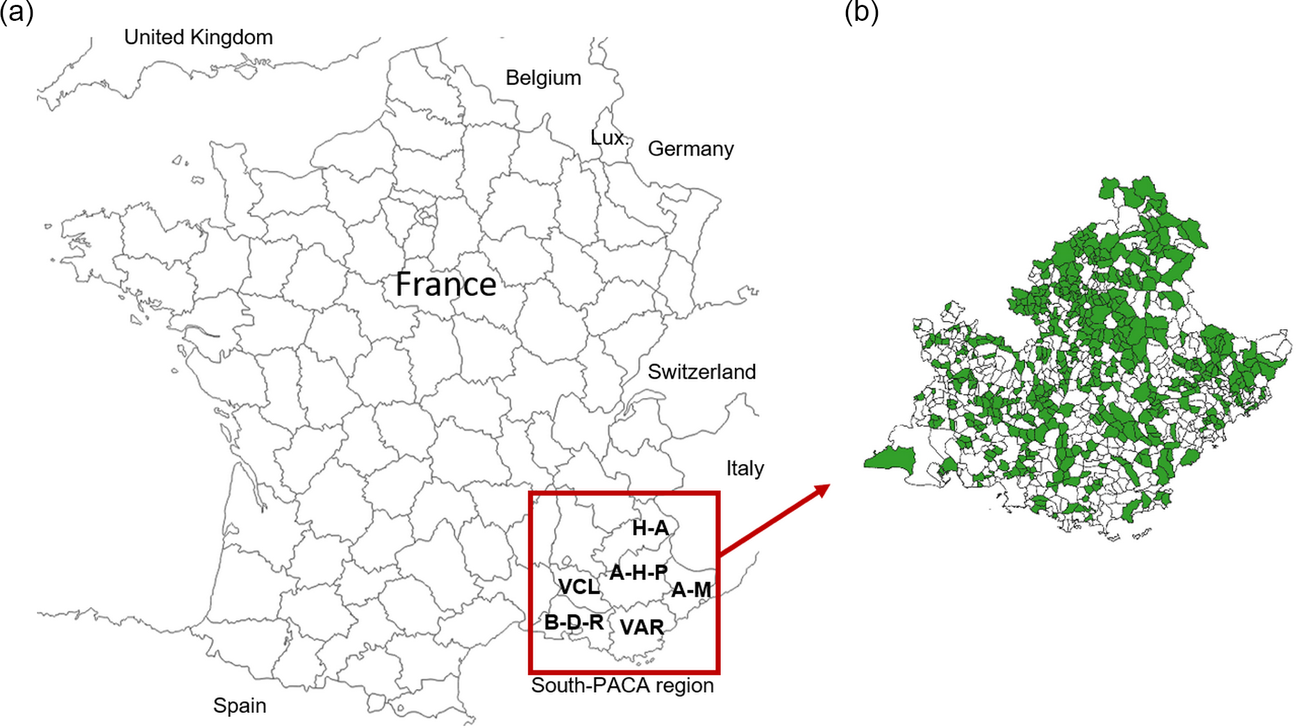
A total of 806,069 birth certificates were recorded from 521 communes with a population of less than 15,000 in the 19th century (Figure 1). The municipalities surveyed were therefore mainly part of the rural area of that period. These records cover the period from 1810 to 1890. As the INSEE ‘surname files’ are made up of birth certificates, they were also chosen in order to facilitate comparison with studies using this corpus. A total of 23,340 surnames were collected. The geographical unit of the study was the canton in order to minimize the differences in the number of births between these cantons since in some communes the number of births could be very low. The communes were therefore grouped according to the canton to which they belonged in 2014, which represented 81 of the 126 cantons in the southern region. In order to assess the population evolution on a micro-evolutionary scale, the dataset was split into three periods of 25 years, each representing one generation (Darlu et al., Reference Darlu, Degioanni and Ruffie1997): P1=1810–1835; P2=1836–1861; P3=1862–1890.
(a) Map of the French departments with the six departments of the Sud-Provence-Alpes-Côte d’Azur region framed: A-H-P: Alpes-de-Haute-Provence; H-A: Hautes-Alpes; A-M: Alpes-Maritimes; B-D-R: Bouches-du-Rhône; Var; VCL: Vaucluse. (b) Map showing the 521 communes studied (in green).
In France, as in most European countries, the patronymic system appeared during the Middle Ages, in around the 10th century. The use of patronymics was progressively regulated by the political power, and its transmission to descendants and its generalization were put in place from the 14th century onwards (Fordant, Reference Fordant1999). The legal standardization of patronymic names took place in several stages. After the French Revolution, the parish registers, drawn up at the parish where baptisms, marriages and burials were recorded, became the registers of civil status, drawn up at the town hall where births, marriages and deaths are recorded (Darlu et al., Reference Darlu, Bloothooft, Boattini, Brouwer, Brouwer and Brunet2012). From 1794 onwards, only the Conseil d’Etat could authorize a change of name and it was forbidden to use names other than those recorded in the civil status register. The appearance of the Family Record Book in 1870 durably consolidated the spelling and patrilineal transmission of surnames in France (Fordant, Reference Fordant1999).
Birth certificates were chosen for this study because they are doubly relevant. Firstly, the INSEE ‘surname files’ are made up of birth certificates and, as a result, working on the same type of certificate made it possible to compare and put into perspective the many existing studies that have used this corpus. Secondly, it is true that the use of surnames raises the issue of the inclusion or exclusion of women’s surnames in the studies as this can change the results (Cheshire, Reference Cheshire2014). However, it has been shown that variation is more likely at small geographical scales (Bowden et al., Reference Bowden, Balaresque, King, Hansen, Lee and Pergl-Wilson2008). At larger scales some studies have shown that excluding women’s surnames does not have a significant impact. This was shown, for example, by Winney et al. (Reference Winney, Boumertit, Day, Davison, Echeta and Evseeva2012) in a 19th century UK-wide study. According to these authors, this is probably due to marriage remaining relatively local during the 19th century in Britain. Thus, the use of birth certificates allows the surnames of women and men before their marriages to be obtained. This was done for the present study because in the 19th century France was under a patriarchal system and marriage led to the change of women’s names.
Statistical analyses
All calculations and statistical analyses were carried out using RStudio® software Version 1.3.1093. First, the evolution of the surname stock was described using descriptive statistics: the number of surnames that remained or disappeared over the three periods and the proportion of individuals they represented. Particular interest was given to surnames registered at a single birth. These, conceptualized by Chareille and Darlu (Reference Chareille and Darlu2013) under the name of ‘hapax’, allow for a very interesting interpretation. Indeed, they can be considered as the last representative of a rare surname, the witness of a migration or a transcription error (Chareille & Darlu, Reference Chareille and Darlu2013).
The evolution of differences between cantons was assessed using the
 ${R_{\rm{st}}}$
index, an estimator used in population genetics (Relethford, Reference Relethford1988; Boattini et al., Reference Boattini, Calboli, Villegas, Gueresi, Franceschi and Paoli2006). For this study it was adapted to the context of surnames and allowed for a measurement of the homogeneity between the subdivisions of the total population studied – here, the cantons (Relethford, Reference Relethford1988; Boattini et al., Reference Boattini, Calboli, Villegas, Gueresi, Franceschi and Paoli2006). This index was calculated for all three periods. A decrease of
 $R_{\rm{st}}$
values across a period reflects an increasing exchange of surnames between the cantons. Conversely, if there are fewer exchanges of surnames the
 ${R_{{\rm{st}}}}$
value will increase (Boattini et al., Reference Boattini, Calboli, Villegas, Gueresi, Franceschi and Paoli2006). The
 ${R_{{\rm{st}}}}$
index was calculated using the
 ${F_{s{\rm{t}}}}$
function of the Biodem package of the R® software, developed by A. Boattini and colleagues.
A study of the distribution of surnames through the theory of isonymy is the main method used in patronymic studies. The evaluation of the isolation of each canton was made possible by the isonymy index
 ${I_{ii}}$
, which is calculated as follows:
 $${I_{ii}} = \mathop \sum \nolimits_k {p_{ki}}^2,$$
where
 ${p_{ki}}$
is the frequency of patronymic k in canton i, and the total is equal to the sum of the squared frequencies of each patronymic k in canton i (Darlu et al., Reference Darlu, Degioanni and Ruffie1997). This mathematical formula calculates the probability of randomly drawing two identical surnames in the same canton; the higher this index, the more isolated the canton (Darlu & Oyharçabal, Reference Darlu and Oyharçabal2006; Carrieri et al., Reference Carrieri, Sans, Dipierri, Alfaro, Mamolini and Sandri2020). Isonymy was calculated using the uri function of the Biodem package of the R® software.
In order to estimate migration on the basis of surnames, the Karlin–McGregor v-index was calculated in accordance with Carrieri et al. (Reference Carrieri, Sans, Dipierri, Alfaro, Mamolini and Sandri2020). This index was developed by Karlin and McGregor (Reference Karlin and McGregor1967) based on the theory of neutral mutation behaviour in finite populations of constant size, in conjunction with the patrilineal transmission of patronyms that can be considered as alleles (Rossi, Reference Rossi2013). This index estimates the ‘mutation rate’ (Darlu & Ruffié, Reference Darlu and Ruffie1992). Since true surname mutations are relatively rare, a high value of v will indicate an influx of new surnames and thus a migratory phenomenon. This index is calculated for each canton i as follows:
 $$v = \alpha /\left( {N - \alpha } \right),$$
where N is the number of people per canton and
 $\alpha = 1/{I_{ii}}$
(Dipierri et al., Reference Dipierri, Alfaro, Scapoli, Mamolini, Rodriguez-Larralde and Barrai2005; Carrieri et al., Reference Carrieri, Sans, Dipierri, Alfaro, Mamolini and Sandri2020).
Patronymic similarities and differences between cantons taken two-by-two were evaluated using Lasker distances. In 1977, Lasker proposed an extension of Crow and Mange’s (Reference Crow and Mange1965) formula to use isonymy as a measure of relatedness between two populations (Lasker, Reference Lasker1977). Lasker’s index
 ${R_{ij}}$
calculates, from surnames, the probability that two human groups i and j have genes in common (Rossi, Reference Rossi2013):
 $${R_{ij}} = {{\sum\nolimits_k {{S_{ki}}} {S_{kj}}} \over {2\sum {{S_i}} \sum {{S_j}} }},$$
where
 ${S_{ki}}$
is the number of occurrences of surname k in canton i and
 ${S_{kj}}$
is the number of occurrences of the same surname in canton j (Colantonio et al., Reference Colantonio, Fuster and Kuffer2007; Roman-Busto & Fuster, Reference Roman-Busto and Fuster2015). The logarithmic transformation of the Lasker index yields the Lasker distance between the two cantons:
 ${L_{ij}} = - {\rm{ln}}\left( {2{R_{ij}}} \right)$
(Rodriguez-Larralde et al., Reference Rodriguez-Larralde, Scapoli, Beretta, Nesti, Mamolini and Barrai1998; Colantonio et al., Reference Colantonio, Fuster and Kuffer2007). The
 ${R_{ij}}$
index is multiplied by two because the Lasker index is equal to twice the isonymy between two groups (Barrai et al., Reference Barrai, Rodriguez-Larralde, Mamolini and Scapoli1999, Reference Barrai, Rodriguez-Larralde, Mamolini, Manni and Scapoli2000; Dipierri et al., Reference Dipierri, Alfaro, Scapoli, Mamolini, Rodriguez-Larralde and Barrai2005). In order to detect isolation by distance, the correlation between Lasker distances and geographical distances was evaluated using the Mantel test, which uses the Monte Carlo method with 9999 permutations. This test was performed with the mantel.randtest function of the R® software package, ade4. The geographical distances between each pair of townships were calculated from the straight-line distance between the township capitals using QGIS® Desktop 3.4.7. A hierarchical ascending classification with Ward’s method was performed using the Lasker distance matrices to create a partition of the townships for each period. The hclust function, with the ‘ward.D2’ method of the R® software package stats was used to obtain the dendrograms. The analysis of the inertia jump of the dendrograms allowed the most homogeneous grouping of the townships possible. The use of cartography, with the software QGIS® Desktop 3.4.7, made it possible to visualize the groups obtained in geographical space.
Results and Discussion
Evolution of the surname stock in Sud-Provence-Alpes-Côte d’Azur
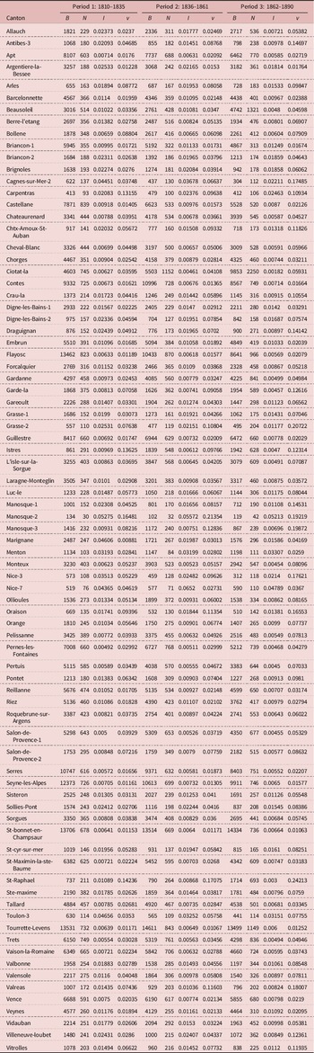
The distribution of surnames within each canton and the parameters calculated from the theory of isonymy are given in Table 1. The 25 most frequent names were studied; ten of them (Martin, Bernard, Robert, Michel, Roux, Bertrand, Bonnet, Blanc, Faure and Girard) were found in the list of 25 most frequent names at the national level of INSEE’s files of patronymic names for the period from 1891 to 1915. The surname Martin is the most frequent in France today and has been since the 19th century (Darlu et al., Reference Darlu, Degioanni and Ruffie1997). But in the corpus studied, the family name Blanc was the most frequent during the three periods with 10,662 occurrences, followed by Roux with 8831 occurrences and Martin (8755 times), which was in third position. They are followed by the surnames Michel (8715), Giraud (6565), Arnaud (5702) and Bernard (4409). These 25 names represent 13.7% of the births registered between 1810 and 1890. They remain essentially the same throughout the three periods, which suggests a certain stability of the population. It is only from the period 1916 to 1940 that the Italian surname Rossi enters the ranking of the 25 most frequent names in the region, according to INSEE’s files of patronymic names.
Distribution of study sample surnames and parameters derived from isonymy theory by time period and Sud-Provence-Alpes-Côte d’Azur cantons

B=number of registered births; N=number of different surnames; I=isonymy; v=Karlin–McGregor’s v-index.
Studying the distribution of frequent and rare surnames is particularly relevant for determining local surnames for genetic studies (Darlu et al., Reference Darlu, Bloothooft, Boattini, Brouwer, Brouwer and Brunet2012; Rossi, Reference Rossi2013); this point is discussed further in the Conclusion section. In France, between 1891 and 1940 the surname Martin was the most frequent surname, and it was present in 81 French departments; Durand was found in 65 departments, Richard in 59 departments and the surname Roux in 44 departments (Darlu et al., Reference Darlu, Degioanni and Ruffie1997). These surnames are defined as polyphyletic because they cannot be considered as specific to one region as they probably have several geographical origins.
In France between 1891 and 1940, 96% of the surnames were present in fewer than ten departments at the same time and two-thirds of them were strictly localized in one department. These surnames are therefore regionally specific markers, and are defined as monophyletic, specific to one region and having only one central origin, as opposed to polyphyletic surnames (Darlu et al., Reference Darlu, Degioanni and Ruffie1997; Rossi, Reference Rossi2013). The existence of these monophyletic surnames can be explained by the old presence of surnames on the French territory and the regional linguistic richness because the surnames are derived from words (Manni et al., Reference Manni, Toupance, Sabbagh and Heyer2005; Rossi, Reference Rossi2013). These patronyms are notably used in population genetics studies (Winney et al., Reference Winney, Boumertit, Day, Davison, Echeta and Evseeva2012; Leslie et al., Reference Leslie, Winney, Hellenthal, Davison, Boumertit and Day2015) in order to improve sampling strategies. They are also used in forensic DNA analysis in court cases (King et al., Reference King, Ballereau, Schurer and Jobling2006). This methodology hypothesizes a relationship between genetic characteristics of the Y chromosome, specific to male lineages, and a monophyletic patronymic that has been patrilineally transmitted for centuries and has a single geographical founder (King et al., Reference King, Ballereau, Schurer and Jobling2006). This hypothesis is not shared by all authors, as there are some very important factors to take into account, such as illegitimate births and abandoned children (Rossi, Reference Rossi2013). However, this type of bias may be limited depending on the temporal and spatial scale of the study or on the initial problem.
For this work, between 1810 and 1890, 23,340 surnames were collected: 11,578 surnames for P1, 12,269 for P2 and 15,469 for P3. This difference in registration is due to the appearance of new surnames in P2 and P3, coupled with the disappearance of other surnames. Only 26.3% of the surnames are common to the three periods but they represent a large part of the births (93.4%) over the entire study of 1810–1890. During the third period, 6898 new surnames were recorded, i.e. 29.5% of the surnames, representing 1.87% of the births. The stock of surnames thus seems to be variable; however, the majority of individuals have names that cross the three periods, suggesting relative stability of the population.
A ‘hapax’ is a name that appears only once in a corpus (Chareille & Darlu, Reference Chareille and Darlu2013). For the three periods, 8299 ‘hapax’ were recorded, i.e. 35.5% of the surnames counted, but they represent only 1% of the registered births. This observation is comparable on a national scale: ‘hapax’ represented 36% of the surnames collected by INSEE between 1891 and 1915 (Darlu et al., Reference Darlu, Degioanni and Ruffie1997). For the first period, 3386 ‘hapax’ were recorded, compared with 3604 for P2 and 5125 for P3. The number of ‘hapax’ thus increased significantly for the third period. Given that ‘hapaxes’ are likely to represent a migration (Chareille & Darlu, Reference Chareille and Darlu2013), their increase in this corpus, particularly in the third period, seems to indicate an increase in migrations. Moreover, these ‘hapax’ had a strong impact on the proportion of names collected, but not on the population as they represented few births. It is therefore possible to say that migration tended to increase, but that its impact on the population’s gene pool was still anecdotal. The estimated
 ${R_{{\rm{st}}}}$
values, respectively for P1
 ${R_{{\rm{st}}}}$
=0.0022, P2
 ${R_{{\rm{st}}}}$
=0.0019 and for P3
 ${R_{{\rm{st}}}}$
=0.0016, decreased across the three periods and especially in the third period. This indicates a homogenization between cantons over time (Boattini et al., Reference Boattini, Calboli, Villegas, Gueresi, Franceschi and Paoli2006). This phenomenon can be explained by the increase in migration, and therefore in the exchange of surnames between cantons, which led to a greater sharing of surnames between cantons. Indeed, the end of the 19th century was marked by great upheavals such as the arrival of the railway in the south-east of France in 1849, which favoured the mobility of individuals. The construction of this means of transport, as well as the development of industry, required a great deal of labour (Gastaut, Reference Gastaut2009). This result is consistent with the increase in ‘hapax’.
Isolation and migration across the century
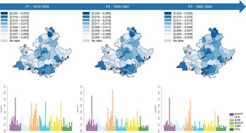
In general, the estimates of inbreeding, presented in Table 1, calculated from the isonymy index, tend to decrease across the three periods. Indeed, according to the cantonal distribution of the estimated isonymy values, presented by canton and by period in the bar charts of Figure 2, the values tend to decrease across the three periods. Thus, the townships became less and less isolated across the three periods. The lowest inbreeding estimates were found in the Durance Valley on the borders of the Vaucluse and Bouches-du-Rhône departments (Figure 2). This area corresponded to a communication corridor known as the Domitian Way, which since its creation during Roman domination has linked Italy to Spain (Temime, Reference Temime1997). The economic role of this valley (as well as the Rhône Valley) is fundamental; it seals the age-old exchanges between north and south through transhumance and various commercial exchanges (Bouvier, Reference Bouvier1979; Gastaut, Reference Gastaut2009).
Maps of the cantonal distribution of the isonymy index by period. The bar graphs represent, for the three periods, the estimated values of the isonymy by canton and coloured according to their department. A-H-P: Alpes-de-Haute-Provence; H-A: Hautes-Alpes; A-M: Alpes-Maritimes; B-D-R: Bouches-du-Rhône; Var; VCL: Vaucluse.

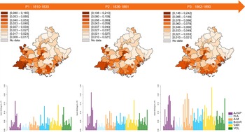
Migration, estimated from the Karlin–McGregor v-index, is presented in Table 1; higher values were found in the south-western quarter of the region (Figure 3). These observations are in line with the unbalanced distribution of today’s population within the southern region (Gastaut, Reference Gastaut2009). In fact, the migratory flows directed towards the coastal cities, rich in industrial centres, have demographically enriched the south-western coastal quarter of the region during the rural exodus. According to the cantonal distribution of the estimated values of the Karlin–McGregor v-index, presented by canton and by period in the bar charts of Figure 3, an increase in values is noticeable across the three periods. Thus, the migration rate increased over the 19th century in the population sample of the southern region studied in this work.
Maps of the cantonal distribution of the Karlin–McGregor v-index by period. The bar graphs represent, for the three periods, the estimated values of the v-index by canton and coloured according to their department. A-H-P: Alpes-de-Haute-Provence; H-A: Hautes-Alpes; A-M: Alpes-Maritimes; B-D-R: Bouches-du-Rhône; Var; VCL: Vaucluse.

Population structure based on Lasker distances
The similarities and differences in surnames between the townships were studied using Lasker distances. These analyses showed that some cantons did not share any surnames. For the first period, the canton of Arles (Bouches-du-Rhône department) and the canton of Menton (Alpes-Maritimes department) did not share any patronymic. For the second period, this was the case for the canton of Menton with the canton of Briançon-2 (department of Hautes-Alpes) and the canton of Digne-les-Bains-2 (department of Alpes-de-Haute-Provence). These cantons were therefore the most different.
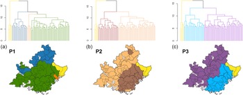
The geographical projection of the groups obtained from the dendrograms (Figure 4) has allowed for a synthesis of the relationships between the cantons according to the periods. The group in yellow in Figure 4a, b and c was maintained throughout the three periods and included five cantons in the eastern-most part of the Alpes-Maritimes: the cantons of Beausoleil, Contes, Menton, Nice-7 and Tourrette-Levens. The singularity of this group and its continuity through the three periods can be explained according to different historical and linguistic phenomena. On the one hand, from a linguistic point of view, the Roya Valley, whose territory extends within the cantons of Contes, Beausoleil and Menton, is closer to the Ligurian dialect of northern Italy (Bouvier, Reference Bouvier1979; Caserio, Reference Caserio2015). It should not be forgotten that language has a particular influence on patronymics, as all patronymics are based on words derived from everyday language (Manni et al., Reference Manni, Toupance, Sabbagh and Heyer2005; Rossi, Reference Rossi2013). On the other hand, the definitive annexation of this geographical area to France was late; 1860 for the County of Nice by referendum (Agulhon & Coulet, Reference Agulhon and Coulet1987; Temime, Reference Temime1997) and 1947 for certain communes located in the Roya Valley following the Second World War and the Treaty of Paris (Baratier et al., Reference Baratier, Duby and Hildesheimer1969; Agulhon & Coulet, Reference Agulhon and Coulet1987).
Dendrograms obtained from a Hierarchical Ascending Classification with Ward’s method using Lasker distances, for each period: (a) Period 1; (b) Period 2; (c) Period 3. The obtained groups were projected on the geographical space.

For the first period, four groups were defined from the dendrogram and are presented in Figure 4a. The largest group, in green, seems to reflect the politics of the County of Provence under the second Capetian house of Anjou-Provence (Baratier et al., Reference Baratier, Duby and Hildesheimer1969; Agulhon & Coulet, Reference Agulhon and Coulet1987), this coinciding with the adoption of patronymics during the Middle Ages. In the north, the department of Hautes-Alpes, formerly Dauphiné, was united with the western territory of Vaucluse, formerly Comté Venaissin, and the canton of Barcelonnette, covering the Ubaye Valley in the north-east of the department of Alpes-de-Haute-Provence. This canton was lost by Provence in 1388 to join the States of Savoy and it was only in 1713, by the Treaty of Utrecht, that it was again attached to Provence (Baratier et al., Reference Baratier, Duby and Hildesheimer1969; Agulhon & Coulet, Reference Agulhon and Coulet1987). The smallest group found around Nice, in orange (Figure 4a) corresponded linguistically to the Nissart dialect (Bouvier, Reference Bouvier1979; Caserio, Reference Caserio2015) and also passed in 1388 under Savoyard suzerainty (Baratier et al., Reference Baratier, Duby and Hildesheimer1969; Agulhon & Coulet, Reference Agulhon and Coulet1987). These findings highlight the multiple identities and histories of the Sud-Provence-Alpes-Côte d’Azur region that do not strictly coincide with current departmental boundaries (Gastaut, Reference Gastaut2009). Indeed, the boundaries of the region and its constituent departments were created on economic factors rather than socio-cultural criteria (Bromberger & Meyer, Reference Bromberger and Meyer2003).
For the second period, three groups were defined from the dendrogram and are presented in Figure 4b. The group located in the south-east, in brown, gathered 27 cantons of the departments of Var, Alpes-Maritimes, Alpes-de-Haute-Provence and one canton of Hautes-Alpes: l’Argentière-la-Bessée. This group seems to be the witness of areas where migratory movements from outside began during the second period of this study (Gastaut, Reference Gastaut2009). Indeed, in the 19th century, tourism and the labour force required for it, experienced a considerable boom on the Côte d’Azur. This was initiated in the 18th century with the first winter resorts of Hyères and Nice attracting English, Germans and Russians (Gastaut, Reference Gastaut2009). In the countryside, particularly in the Var and Alpes-Maritimes, waves of immigrant workers came to supplement the lack of labour left by the rural exodus from the 1830s to 1840s (Gastaut et al., Reference Gastaut, Rinaudo, Dahhan, Véglia, Folliet and Sagatni2008). The labour force, essentially Italian, was much sought after for viticultural or agricultural work because of their low wages (Gastaut et al., Reference Gastaut, Rinaudo, Dahhan, Véglia, Folliet and Sagatni2008). The attachment of the canton of Argentière-la-Bessée in the Hautes-Alpes to the south-east group was, however, surprising at first glance. But it can be explained by the activity of its silver mine, which became notable and prosperous from 1855 onwards, employing up to 500 workers (Ancel, Reference Ancel1997). For the group located to the west, in beige (Figure 4b), it gathered 49 cantons of Bouches-du-Rhône, Vaucluse, Alpes-de-Haute-Provence, Hautes-Alpes and the canton of La Crau in Var. This grouping seems to be the witness of an intra-regional migratory movement (Alpine, peasants) directed towards the south-western coast (Baratier et al., Reference Baratier, Duby and Hildesheimer1969, Agulhon & Coulet, Reference Agulhon and Coulet1987; Temime, Reference Temime1997; Gastaut et al., Reference Gastaut, Rinaudo, Dahhan, Véglia, Folliet and Sagatni2008; Gastaut Reference Gastaut2009). Indeed, there has always been a co-dependence between the north, providing seasonal workers, and the south, providing blue-collar jobs thanks to the development of industry, within the Sud-Provence-Alpes-Côte d’Azur region (Baratier et al., Reference Baratier, Duby and Hildesheimer1969; Agulhon & Coulet, Reference Agulhon and Coulet1987; Temime, Reference Temime1997; Gastaut, Reference Gastaut2009).
For the third period, three groups were defined from the dendrogram and are presented in Figure 4c. The blue group in the east included 26 cantons in the Var and Alpes-Maritimes, one canton in Alpes-de-Haute-Provence and the canton of La Ciotat in Bouches-du-Rhône, which in the previous period was part of the western group. The western group in blue (Figure 4c) included 50 cantons from Bouches-du-Rhône, Vaucluse, Alpes-de Haute-Provence and Hautes-Alpes. As for the canton of Argentière-la-Bessée, for the third period, it was no longer attached to the eastern group, probably because its silver mining activity declined from 1870 and stopped temporarily in 1881 (Ancel, Reference Ancel1997). At the same time, the canton of La Crau in the Var and La Ciotat in the Bouches-du-Rhône were attached to the western group in the third period. These two coastal cantons gradually welcomed Italian workers. Indeed, the commune of La Ciotat, which is the chief town of the canton of La Ciotat, is known for the development of its shipyards at the end of the 19th century (Gastaut, Reference Gastaut2009).
These observations seem to depict an Italian migratory influence from east to west that will become a so-called ‘mass’ migration from the end of the 19th century (Temime, Reference Temime1997). Indeed, immigrant workers settled everywhere in the region and particularly in the highly industrialized urban areas from the end of the 19th century (Gastaut, Reference Gastaut2009). Of course, it is not possible to say, with the method used, whether the groups obtained in the third period are strictly the result of the evolution of the groups of the second period. But the change in population structures across the three periods indicates a fairly significant modification of the patronymic stock to the point of changing the relationships between the cantons (Chareille & Darlu, Reference Chareille and Darlu2013). Obviously, the fact that cities with a population of more than 15,000 inhabitants, such as Marseille and Nice, were not taken into account in this study conditions these results. The population mix present in these urban centres would have disrupted the study of relations and structures in rural areas, as these cities were marked by the presence of Italian labour from the mid-19th century (Baratier et al., Reference Baratier, Duby and Hildesheimer1969; Agulhon & Coulet, Reference Agulhon and Coulet1987; Temime, Reference Temime1997; Gastaut et al., Reference Gastaut, Rinaudo, Dahhan, Véglia, Folliet and Sagatni2008; Gastaut, Reference Gastaut2009).
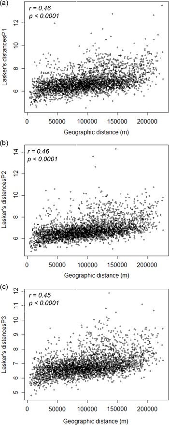
For the Mantel test, the r correlations between Lasker distances and geographical distances (r=0.46 for P1 and P2 and r=0.45 for P3) were positive and significant (p<0.0001) for all periods. The scatterplot in Figure 5 shows a linear and positive relationship between the geographical distance matrix and the patronymic distance matrix for all three periods. Thus, the greater the geographical distance between the cantons, the greater the patronymic distance. The geographical distance seems to have had an influence on the differentiations of the patronymic stocks between the cantons.
Variation of the Lasker distance with the geographical distance (in metres) between the 81 cantons studied in the Sud-Provence-Alpes-Côte d’Azur region by period: (a) Period 1; (b) Period 2; (c) Period 3.

Conclusion
With a multidisciplinary approach, this study has provided access to the population structures of the Sud-Provence-Alpes-Côte d’Azur region before the upheavals brought about by the migratory movements of the 20th century. Of course, this region has always welcomed migration, but in the 19th and 20th centuries, it became a major axis in France (Gastaut, Reference Gastaut2009). This phenomenon began in the middle of the 19th century and had an impact on the structures of the population, which was mainly rural, that is studied here. The three-period approach was able to show this evolution; the structures obtained from groups linked to geographical areas impregnated with different historical, linguistic and geographical processes. The first period reflects an Ancien Régime Provence, while the structures found for P2 and P3 strongly echo the descriptions provided by the historian Gastaut (Gastaut et al., Reference Gastaut, Rinaudo, Dahhan, Véglia, Folliet and Sagatni2008; Gastaut Reference Gastaut2009) on the different types of migrations existing within the region.
The socioeconomic changes of the 19th century completely modified the patronymic structures of the southern region. The decrease in inbreeding estimates
 $\;({R_{{\rm{st}}}}$
values), the increase in Karlin and McGregor’s ‘mutation rate’ v and ‘hapax’, are consistent with increasing migration and population mixing over the chronological period studied. These trends are most pronounced in the third period, which coincides with the onset of the rural exodus, the Industrial Revolution and international migration in the South.
This study makes it possible to understand the beginnings of a so-called ‘mass’ migration wave described by historians (Temime, Reference Temime1997; Gastaut, Reference Gastaut2009). Thanks to the analogy between isonymic and genetic structures, it provides biological confirmation of historical facts and has made it possible to evaluate the importance of migratory flows within the region. This work highlights the singularity of the eastern part of the Alpes-Maritimes compared with the rest of the region, which is maintained throughout the three periods. This singularity will continue into the 21st century according to a study by Scapoli et al. (Reference Scapoli, Goebl, Sobota, Mamolini, Rodriguez-Larralde and Barrai2005).
The study of this geographical area and the historical depth proposed can be relevant to a wide range of research applications in public health and population genetics. Initially, collaboration with the Etablissement Français du Sang (EFS) could allow the identification of rare genetic variants (blood systems, HLA) in this geographical area. This knowledge is essential in a public health strategy (Kristiansson et al., Reference Kristiansson, Naukkarinen and Peltonen2008) that aims to improve blood transfusions by identifying geographical areas capable of supplying rare blood groups. The Sud-Provence-Alpes-Côte d’Azur region is a very good candidate for rare blood group research because of its geographical environment which is conducive to isolation (Chiaroni et al., Reference Chiaroni, Chevé, Berland-Benhaïm and LeCoz2016). More than a century after the discovery of the ABO blood group, blood transfusion remains a major therapy that saves tens of thousands of patients per year (Bodmer, Reference Bodmer2015) and the anthropological interest of erythrocyte blood groups can provide valuable information in this field (Marchini et al., Reference Marchini, Cardon, Phillips and Donnelly2004). Secondly, the relevance of the use of surnames as a geodemographic indicator is undeniable (Darlu et al., Reference Darlu, Bloothooft, Boattini, Brouwer, Brouwer and Brunet2012, Cheshire, Reference Cheshire2014). Indeed, the identification of locally rooted surnames makes it possible to improve sampling strategies for population genetics by targeting specific geographical areas (Darlu et al., Reference Darlu, Bloothooft, Boattini, Brouwer, Brouwer and Brunet2012). In particular, in the collaborative work of Winney et al. (Reference Winney, Boumertit, Day, Davison, Echeta and Evseeva2012) and Leslie et al. (Reference Leslie, Winney, Hellenthal, Davison, Boumertit and Day2015), this methodology has enabled the identification of genetic clusters within Britain which they have been able to link to historical events dating back to the Middle Ages. This approach allows the identification of genetic isolates from the past and population structures that have been altered or disappeared today (Darlu et al., Reference Darlu, Bloothooft, Boattini, Brouwer, Brouwer and Brunet2012). In some cases, the correlation between Y-chromosome characteristics and surname has even proved fruitful in a forensic context (King et al., Reference King, Ballereau, Schurer and Jobling2006). It therefore seems that although we are in the era of the study of complete genomes, these genetic approaches through patronyms allow for indispensable interdisciplinary exchanges in the understanding of human populations.
Funding
The study was part of the doctoral project of the first author, who obtained doctoral funding from the Sud-Provence-Alpes-Côte d’Azur region and the French Blood Establishment (EFS Sud-Provence-Alpes-Côte d’Azur -Corse).
Conflicts of Interest
The authors have no conflicts of interests to declare.
Ethical Approval
The authors assert that all procedures contributing to this work comply with the ethical standards of the relevant national and institutional committees on human experimentation and with the Helsinki Declaration of 1975, as revised in 2008.