4.1 Comparison of experimental and analytical results

We first compare the analytical and experimental results for the set of test cases given in table 1. In figure 7 we present results for the measured acoustic sound pressure levels at each of the 11 microphone locations, for aerofoils with 6 % or 12 % thickness that are modified forms of standard NACA 4-digit aerofoils, with leading-edge nose radii described by (3.1). Two low-Mach-number mean flow velocities are used corresponding to $U^{\ast }=20,80~\text{m}~\text{s}^{-1}$ ( $M=0.06,0.24$ ), and two non-dimensionalised frequencies, $k=2.5,5$ .

The total noise radiated by the aerofoil located within a turbulent flow is dominated by leading-edge noise at these chosen frequencies but by trailing-edge noise at higher frequencies. As it is very difficult to measure leading-edge noise and trailing-edge self-noise separately, our experimental analysis was limited to the frequency region where the interaction noise dominates trailing-edge self-noise. Figure 5 shows the influence of self-noise on the total noise spectra. The spectra of radiated noise due to trailing-edge self-noise alone is obtained by removing the turbulence grid. Sound power levels are plotted against a non-dimensional frequency ( $k$ ) for aerofoils with two different thicknesses for the highest flow speed of $M=0.24$ . It is observed that the thicker aerofoil has lower interaction noise and the self-noise starts dominating the total noise at a relatively lower frequency compared to the thinner aerofoil. The non-dimensional frequency ( $k$ ) where self-noise starts to dominant the total noise for NACA 0012 is around 6. Whereas for NACA 0006 it is greater than 10. These frequencies are a function of incoming turbulence intensity, where in our present study it is approximately 2.5 %. Below these frequencies the difference between total noise and trailing-edge self-noise is greater than 5 dB, suggesting the dominance of trailing-edge noise on total noise is negligible. Hence, in the frequency range considered in this present study, leading-edge noise is the main contributor to the total far-field noise measured.

Figure 6.

Legend for experimental and analytical results in figures 7 and 8, with $I$ defined in (3.1). The corresponding values of $m$ can be found in table 1 for aerofoil thicknesses of 6 % and 12 %.

Figure 7.

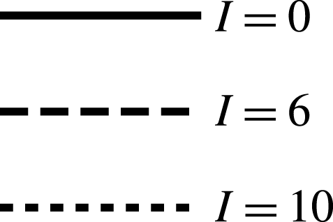
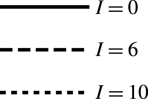
Sound pressure level measured experimentally against polar angle $\unicode[STIX]{x1D703}$ . Legend given in figure 6.

For the highest frequency, $k=5$ , and 12 % thickness we see in figure 7 that as nose radius increases ( $I$ increases), the magnitude of the acoustic pressure decreases. The level of reduction is decreased for the higher mean flow. It is known from Chaitanya et al. (Reference Chaitanya, Gill, Narayanan, Joseph, Vanderwel, Zhang and Ganapathisubramani2015) that the ratio of nose radius, $R_{e}$ (which contains both $\unicode[STIX]{x1D716}$ and $I$ dependence), to the hydrodynamic wavelength, $U^{\ast }/k^{\ast }$ , is an important factor and defines the extent of gust distortion, which in turn governs the far-field noise. With the increase of jet velocity, we observe a decrease in $k^{\ast }R_{e}/U^{\ast }$ , resulting in a decrease in level of noise reduction. For a thinner overall aerofoil, 6 % thickness, we see the same trends as the 12 %-thickness aerofoils, although the reduction in magnitude of the overall SPL is lower for an aerofoil of 6 % thickness than 12 % thickness. At lower frequencies, $k=2.5$ , the trend continues; aerofoils with larger nose radii generate less far-field noise, however the difference in SPL for the thinnest aerofoil (6 %) at the highest mean flow speed ( $80~\text{m}~\text{s}^{-1}$ ) is very small. We can summarise these results by returning to the factor, $k^{\ast }R_{e}/U^{\ast }$ ; greater values of $k^{\ast }R_{e}/U^{\ast }$ produce greater noise reductions.

We compare the experimental results of figure 7(a–h) to the analytical results in figure 8, which plot the far-field acoustic directivity for low-Mach-number flow ( $M=0.06,0.24$ ) at two different frequencies $k=2.5,5$ . The directivity, $D(\unicode[STIX]{x1D703})$ , is defined in (2.29), and is restricted in figure 8 to the experimentally measured range, $\unicode[STIX]{x1D703}\in [40^{\circ },140^{\circ }]$ .

Analytically we focus on gusts with zero spanwise wavenumber, $k_{3}=0$ and $A_{3}=0$ , since the experimental set-up is fundamentally two-dimensional. The dominant contributor to leading-edge noise for symmetric aerofoils in homogeneous isotropic turbulence arises from purely transverse disturbances ( $k_{n}=A_{n}=0$ ) (Gill, Zhang & Joseph Reference Gill, Zhang and Joseph2014), thus we take $k_{n}=0$ .

We require the gust to be solenoidal, therefore $A_{t}+A_{n}k_{n}\unicode[STIX]{x1D6FD}_{\infty }=0$ , and to ensure we ensure the magnitude of the incident gust vector far upstream is constant we set $A_{t}^{2}+A_{n}^{2}=1$ . Specifying $k_{n}$ thus completely determines the incident gust.

Figure 8.

Analytic far-field acoustic directivity, $\log _{10}|D(\unicode[STIX]{x1D703})|$ , against polar angle $\unicode[STIX]{x1D703}$ . Legend given in figure 6.

We observe a good agreement between the experimental and analytical trends, which overall indicate that an increased nose radius (blunter nose) reduces noise.

The analytical and experimental results agree well for $k=5$ , with the NACA 0006 indicating a linear reduction of noise with increasing nose radius, whilst the NACA 0012 results show the $I=10$ result can produce more noise that the $I=6$ .

The analytic $k=2.5$ results show a weaker effect of altering nose radius on the noise produced, in agreement with the experimental measurements. The analytic results predict an increase of noise for a very blunt nose ( $I=10$ ) compared to a very sharp nose ( $I=0$ ) in the upstream direction ( $\unicode[STIX]{x1D703}=\unicode[STIX]{x03C0}$ being the directly upstream direction) except for 6 % thickness in the lowest speed flow, $M=0.06$ (figure 8 f). This feature is only shown in the experimental results at the final upstream microphone location for the 12 % aerofoils. We note the analytic results neglect transition regions which heavily influence an $O(k^{-1/2})$ polar angle region directly upstream and downstream (Ayton Reference Ayton2016). This is equivalent to an angle of $36^{\circ }$ , thus we would expect potential inaccuracies at the extremities of the analytic results for $k=2.5$ . Further, the amplitude errors elsewhere in the analytic solution are $O(k^{-1})$ as we assume $k\gg 1$ . Thus we expect bigger errors in the lower-frequency analytic results than the higher-frequency analytic results. We also see a difference in overall pattern between the analytically predicted SPL for $k=2.5$ , $M=0.06$ – the analytic results do not decrease with increasing $\unicode[STIX]{x1D703}$ . We also attribute this to a lack of inclusion of a transition region for the larger $\unicode[STIX]{x1D703}$ values.

4.2 Mechanisms for noise generation

Having determined the trends experimentally for increasing nose radius we see good agreement with the analytical solution. We now use our analytical leading-edge solution, equation (2.21), to investigate the individual flow features that could impact the change of noise generation when nose radius is altered. We do so by considering the individual terms in the leading-edge solution given by $L_{1,2,3c_{1,2,3},3p}(\unicode[STIX]{x1D703})$ , as each describes a different physical process occurring in the governing equations.

We previously considered only $k_{n}=0$ ; however, to get a full picture of the effects of all leading-edge terms we shall consider two cases here, $k_{n}=0,1$ . We also wish to determine the effects of higher-Mach-number flow, which are practically relevant to the leading-edge noise problem, but due to facility restrictions could not be investigated experimentally. We hence consider both low- and high-Mach-number flows analytically, $M=0.3,0.6$ . Finally, since a higher frequency leads to a greater difference in noise generation with varying nose radius, and the analytic results become increasingly accurate with increasing frequency, we shall focus on two high-frequency cases, $k=5,10$ .

We notice that $k_{n}$ does not explicitly feature in the terms $L_{3p,c_{i}}$ in the leading-edge solution (2.21), and $A_{n}$ is an overall factor, since the $H_{3}$ solution considers the distortion of the flat-plate acoustics through a locally non-uniform flow at the nose – a process that is independent of the gust. Therefore, the effect of altering $k_{n}$ on these terms will be an overall scaling factor only (since altering $k_{n}$ alters the coefficient $A_{n}$ ). The main influence of $k_{n}$ lies in the $L_{1,2}$ terms which represent the effects of the changing surface normal direction on blocking gust velocities, and effects of the volume source generated by the gust in the locally non-uniform flow at the nose, respectively. Both processes are clearly dependent on the gust normal wavevector component. We therefore present $|L_{1,2}|$ for both $k_{n}=0,1$ , but $|L_{3p,c_{1,2,3}}|$ only for $k_{n}=0$ , in figures 10 and 11 when $M_{\infty }=0.6$ , and $|L_{1,2,3p,3c_{i}}|$ for $k_{n}=0$ at $M_{\infty }=0.3$ in figure 12. We consider five different leading-edge geometries, defined by $m=0.2$ , $0.3$ , $0.5$ , $0.7$ , $0.8$ , and all analytic plots share the legend shown in figure 9.

Figure 9.

Legend for analytic results.

Figure 10.

Polar plot of $L_{1,2,3p,3c_{1,2,3}}$ for different leading-edge geometries, for $M_{\infty }=0.6$ , and $k_{n}=0$ . Legend given in figure 9.

Figure 11.

Polar plot of $L_{1,2}$ for different leading-edge geometries, for $M_{\infty }=0.6$ , and $k_{n}=1$ . Legend given in figure 9.

In figure 10 ( $k_{n}=0,M_{\infty }=0.6$ ), figure 11 ( $k_{n}=1,M_{\infty }=0.6$ ) and figure 12 ( $k_{n}=0$ , $M_{\infty }=0.3$ ) the scaling parameter $\unicode[STIX]{x1D716}a_{0}k^{1-m}$ is neglected, therefore we have removed the thickness and frequency scaling of the locally non-uniform mean flow at the nose (which as $m$ increases to give a sharper nose, reduces in magnitude). Having removed this asymptotic parameter, for each given $m$ , the relative magnitude of the results in figures 10–12 indicate the level of influence of that term in the total leading-edge acoustic pressure. We see that by increasing $m$ , the influence of $L_{3c_{1,2,3}}$ reduces, but the influence of $L_{2,3p}$ increases. This indicates that source terms (the volume source for $L_{2}$ , and the flat-plate acoustics for $L_{3p}$ ) become more important as the leading edge is sharpened.

By considering the boundary condition for $H_{1}$ , equation (2.15b ), we see it consists of normal and tangential gust terms, $A_{n,t}$ , multiplied by directional terms, $\sin (m\unicode[STIX]{x03C0})$ and $\cos (m\unicode[STIX]{x03C0})$ . In the case of $k_{n}=0$ , the outer limit, $L_{1}$ shown in figure 10(a), has no tangential component ( $A_{t}=0$ ), thus the solution depends only on the (vertical) directional term $\sin (m\unicode[STIX]{x03C0})$ . The magnitude of $L_{1}$ hence varies proportionally to $|\sin (m\unicode[STIX]{x03C0})|$ as $m$ varies, thus unlike $L_{2,3}$ there is no trend of overall increase or decrease with increasing $m$ . When $A_{t}\neq 0$ in figure 11(a), we see $L_{1}$ decreases in magnitude for increasing $m$ . Here the variation in size of the directional terms $\sin (m\unicode[STIX]{x03C0})$ and $\cos (m\unicode[STIX]{x03C0})$ are less important, and the overall scaling in $m$ arising from the Fourier transform of $\unicode[STIX]{x1D6F7}^{m-1}$ , which represents the rate of slowing of the steady flow on approach to the frontal stagnation point, dominates. A smaller value of $m$ indicates a blunter nose, and hence a greater rate of slowing of the flow and a larger magnitude of the solution $L_{1}$ .

Figure 11(b) illustrates the effects of an asymmetric incident field on a symmetric aerofoil, as the gust distortion at the nose depends on the angle at which it approaches the aerofoil. The overall trend as $m$ varies agrees with the symmetric $k_{n}=0$ case in figure 10(b), indicating for $k_{n}\neq 0$ the volume source term is still promoted as $m$ increases.

Figure 12.

Polar plot of $L_{1,2,3p,3c_{1,2,3}}$ for different leading-edge geometries, for $M_{\infty }=0.3$ , and $k_{n}=0$ . Legend given in figure 9.

We now consider the magnitudes of the $L_{1,2,3p,3c_{1,2,3}}$ for low Mach number, $M_{\infty }=0.3$ , in figure 12 and compare to the results for moderate Mach number, $M_{\infty }=0.6$ (figure 10). Overall all directivities are stretched horizontally for $M_{\infty }=0.6$ compared to $M_{\infty }=0.3$ due to Doppler effects, but trends when varying $m$ for each individual directivity function remain the same. We also see that the relative sizes of certain $L_{1,2,3p,3c_{1,2,3}}$ are decreased; in particular, at low Mach number, $L_{1,3p}$ are substantially smaller than at moderate Mach number. Thus at low Mach number, any effects of $L_{1,3p}$ will be less evident in the total far-field acoustic solution than at moderate Mach number.

Figure 13.

Full aerofoil shapes (with chord length $2$ ) used for different leading-edge geometries $y\sim \unicode[STIX]{x1D716}a_{0}x^{m}$ . Legend given in figure 9.

Finally, we plot the full pressure directivity, $|D(\unicode[STIX]{x1D703})|$ , as given by (2.29). We focus specifically on $k_{n}=0$ gusts. All aerofoils have the same maximum thickness, but varying leading-edge geometry, as can be seen in figure 13, produced by taking the standard NACA 4-digit profile but altering the first term from $x^{0.5}$ to $x^{m}$ . To ensure the maximum thickness is fixed across all aerofoils, different values of $a_{0}$ have to be chosen for different values of $m$ . These are given in table 2. We see from this table that the parameter $\unicode[STIX]{x1D716}a_{0}k^{1-m}$ is similar across the range of $m$ chosen for our two chosen frequencies, $k=5,10$ , therefore any effects seen altering the far-field noise are not caused purely by the changing scaling of the steady flow at the nose, $q$ (2.3).

Table 2.

Table of values of $m$ and $a_{0}$ chosen to ensure equal total aerofoil thickness $\unicode[STIX]{x1D716}=0.06$ for a modified NACA 4-digit profile, and asymptotic parameter $\unicode[STIX]{x1D716}a_{0}k^{1-m}$ with $k=5,10$ .

Figure 14 gives the directivity for $k_{n}=0$ and $M_{\infty }=0.3$ at two gust frequencies, $k=5,10$ ; we see that as the aerofoil nose becomes blunter (decreasing $m$ ) the noise reduces across all angles for both frequencies (as also seen in figure 8 for the comparison with experimental data). To cause this we would expect source terms, indicated by solutions $L_{2}$ and $L_{3p}$ , to add to the total noise, which is justified by the consistent trends seen in figures 10(b,c) and 14. Terms $L_{3c_{1,2,3}}$ likely subtract. We see similar results at frequency $k=5$ as those seen at $k=10$ , since the only influence of the frequency on the directivity is in the asymptotic scaling parameter $\unicode[STIX]{x1D716}a_{0}k^{1-m}$ , which affects the total size of the added thickness-related terms, but not the individual effects seen by varying $m$ in the $L_{1,2,3}$ terms.

At higher Mach number, $M_{\infty }=0.6$ , figure 15 for frequencies $k=5,10$ shows more significant modulation of the solution, due to the greater interference between leading- and trailing-edge fields. At both frequencies we see an increase of noise in the upstream region for a very blunt leading edges ( $m=0.2$ ), although elsewhere the noise is reduced as $m$ is decreased. This upstream increase was observed experimentally in figure 7 for a 12 % total thickness aerofoil in low-Mach-number flow. Analytically the upstream increase is greatest for $k=10$ . By increasing the Mach number we have increased the relative importance of terms $L_{1,3p}$ . We can determine that the $L_{1}$ term subtracts from the flat-plate term, $L_{0}$ , by considering the phase difference between $L_{1}$ and $L_{0}$ . Therefore, the rate of slowing of the flow on approach to the stagnation point decreases far-field noise. Since $L_{1}$ subtracts from the flat-plate term we do not expect this term to be contributing to the increase of noise upstream. Instead we notice that the $L_{3p}$ term for $M_{\infty }=0.6$ in figure 10(c) shows an increase in magnitude in the upstream region as $m$ is reduced, which is more extreme than the distortion to the upstream direction seen for $M_{\infty }=0.3$ in figure 12(c). We therefore attribute the increase in noise upstream seen in figure 15 to the increased upstream distortion seen in $L_{3p}$ at higher Mach numbers, which as a source term adds to the total noise. Specifically, $L_{3p}$ accounts for the distortion of the volume source generated by the flat-plate term due to the locally non-uniform mean flow around the nose. This locally non-uniform flow is directed upstream, and increases with the bluntness of the nose – thus as we decrease $m$ we see a distortion of the acoustics from $L_{3p}$ to the upstream direction, that is increasingly evident at higher Mach numbers.

Figure 14.

Polar plot of the far-field acoustic directivity, $|D(\unicode[STIX]{x1D703})|$ , for different leading-edge geometries, for $k_{n}=0$ , $M_{\infty }=0.3$ . Legend given in figure 9.

Figure 15.

Polar plot of the far-field acoustic directivity, $|D(\unicode[STIX]{x1D703})|$ , for different leading-edge geometries, for $k_{n}=0$ , $M_{\infty }=0.6$ . Legend given in figure 9.