1 Introduction
‘Moonpools’ are vertical openings, from deck to keel, through the hulls of some ships and offshore structures, such as drillships or offshore construction vessels (OCVs). ‘Gaps’ are the narrow spaces in between two ships moored side by side, or between a ship and a quay. Moonpools and gaps are prone to resonance problems, under outer wave action and wave-induced motion of the floating supports.
Resonant modes in moonpools consist in sloshing modes, alike in tanks, and in an additional mode known as the piston, or pumping, mode, where the entrapped water heaves up and down more or less like a solid body. When resonating, these modes hinder marine operations such as drilling and installation of subsea equipment. Due to the increase in size of moonpools in drillships and in OCVs (to install larger and larger subsea equipment), recently much attention has been given to moonpool resonance (for example, see Faltinsen, Rognebakke & Timokha Reference Faltinsen, Rognebakke and Timokha2007; Faltinsen & Timokha Reference Faltinsen and Timokha2015; Yoo et al. Reference Yoo, Kim, Lee, Kim and Yang2017). With the development of offshore LNG (Liquefied Natural Gas) activity, interest has also increased in gap resonance, that limits ship-to-ship offloading operations, for instance from floating liquefied natural gas (FLNG) to LNG-carrier, or from LNG-carrier to floating storage regasification unit (FSRU). Recent comprehensive reviews on gap resonance can be found, for example, in Sun, Eatock Taylor & Taylor (Reference Sun, Eatock Taylor and Taylor2010) or Zhao et al. (Reference Zhao, Wolgamot, Taylor and Eatock Taylor2017).
In an earlier paper (Molin Reference Molin2001), a theoretical model, based on linearized potential flow theory, was proposed to derive the natural frequencies and associated modal shapes of the piston and sloshing modes in rectangular moonpools. This model was based on simplifying assumptions: the floating support is motionless, the water depth is infinite, and the beam and length of the support are taken to the limit where they are of infinite extent. The geometry is then equivalent to a rectangular opening in a rigid ice-sheet. The fluid domain is divided into two sub-domains: the moonpool and a semi-infinite domain below the keel line. Eigenfunction expansions are used to describe the velocity potential inside the moonpool. The connection with the flow in the lower fluid domain is ensured via an integral equation relating the velocity potential to its vertical derivative, at the base of the moonpool. Then an eigenvalue problem is formulated and solved numerically.
A drawback of this model is that it cannot apply to the finite depth case. Drillships and OCVs usually operate in large water depths. However, side-by-side configurations are often encountered in restricted water depth, for instance in the case of a LNG-carrier moored along a FSRU or along a gravity-based structure (GBS). Moreover the infinite beam assumption leads to the natural frequency of the piston mode being underestimated.
In this paper a slightly different approach is proposed, that applies to the finite depth case, and where the horizontal dimensions of the floating supports are finite. In this model, eigenfunction expansions (for example, see Linton & McIver Reference Linton and McIver2001) are used both in the moonpool (or gap) and in a lower subdomain bounded by the seafloor, the hull, and a fictitious outer cylinder (rectangular or circular) where the velocity potential is taken to be nil. This is a somewhat gross condition to ensure connection with the outer domain; however, as will be seen, it leads to rather good results.
The organization of the paper is as follows: the circular moonpool case is considered first, in infinite depth following the previous method of Molin (Reference Molin2001), then in finite depth following the new model. Both axisymmetric and antisymmetric resonant modes are considered. In the finite depth and finite outer radius case, the obtained natural frequencies are validated through comparisons with results from the diffraction code WAMIT. In the second part of the paper, the rectangular gap case is tackled, and comparisons are made with numerical results from Molin et al. (Reference Molin, Remy, Camhi and Ledoux2009). Finally the rectangular moonpool case is addressed, and applications are made to a barge with a large moonpool, and to a floating foundation for a wind turbine. In all cases simple formulas are proposed, based on so-called single-mode approximations, that give first estimates of the resonant frequencies. It is believed that these formulas can be helpful to offshore engineers for preliminary designs.
Circular moonpool. Geometry.

2 Circular moonpool
2.1 Infinite depth
In this section, as in Molin (Reference Molin2001), we assume the water depth to be infinite, and the structure to be of infinite extent in the horizontal direction. The geometry is therefore equivalent to a circular opening in the middle of an infinite ice-cover.
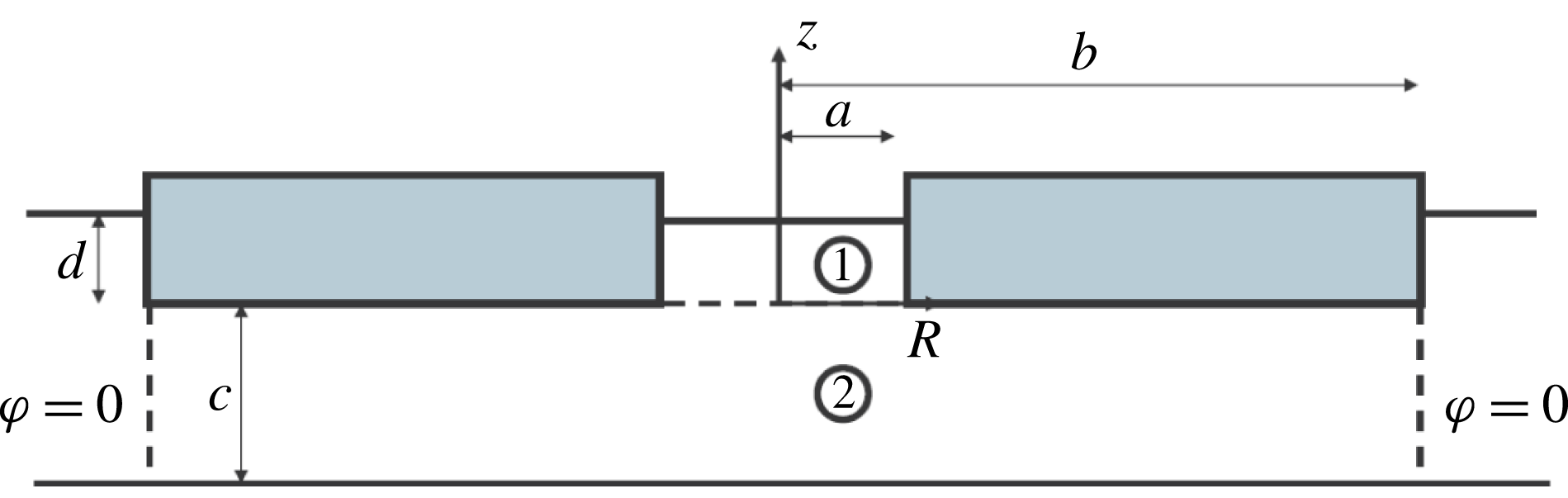
Figure 1 illustrates the geometry: the radius of the moonpool is
 $a$
, its draft is
 $d$
. The origin of the coordinate system is on the axis of symmetry, at the keel level. Natural modes are eigensolutions of the following boundary value problem:
 $$\begin{eqnarray}\displaystyle & \displaystyle \unicode[STIX]{x0394}\unicode[STIX]{x1D711}=0,\quad 0\leqslant R\leqslant a,\;0\leqslant z\leqslant d & \displaystyle\end{eqnarray}$$
 $$\begin{eqnarray}\displaystyle & \displaystyle \unicode[STIX]{x1D711}_{R}=0,\quad R=a,\;0\leqslant z\leqslant d & \displaystyle\end{eqnarray}$$
 $$\begin{eqnarray}\displaystyle & \displaystyle g\,\unicode[STIX]{x1D711}_{z}-\unicode[STIX]{x1D714}^{2}\,\unicode[STIX]{x1D711}=0,\quad 0\leqslant R\leqslant a,\;z=d, & \displaystyle\end{eqnarray}$$
plus a matching condition with the flow in the lower fluid domain which, under the assumptions of infinite depth and infinite horizontal extent of the support, takes the form (Molin Reference Molin2001)
 $$\begin{eqnarray}\displaystyle & \displaystyle \unicode[STIX]{x1D711}(x,y,0)=\frac{1}{2\unicode[STIX]{x03C0}}\int \int _{S}\frac{\unicode[STIX]{x1D711}_{z}(x^{\prime },y^{\prime },0)}{\sqrt{(x-x^{\prime })^{2}+(y-y^{\prime })^{2}}}\,\text{d}x^{\prime }\;\text{d}y^{\prime }, & \displaystyle\end{eqnarray}$$
with
 $S$
the disc
 $0\leqslant R^{\prime }\leqslant a$
,
 ${R^{\prime }}^{2}={x^{\prime }}^{2}+{y^{\prime }}^{2}$
. (In (2.2) and (2.3) the subscripts
 $_{R}$
and
 $_{z}$
mean partial derivatives.)
Here the linearized velocity potential
 $\unicode[STIX]{x1D6F7}(x,y,z,t)$
(or
 $\unicode[STIX]{x1D6F7}(R,z,\unicode[STIX]{x1D703},t)$
in cylindrical coordinates) is supposed to be harmonic in time at the still unknown frequency
 $\unicode[STIX]{x1D714}$
:
 $\unicode[STIX]{x1D6F7}(x,y,z,t)=\unicode[STIX]{x1D711}(x,y,z)\;\cos (\unicode[STIX]{x1D714}t+\unicode[STIX]{x1D713})$
.
The reduced velocity potential
 $\unicode[STIX]{x1D711}(R,z,\unicode[STIX]{x1D703})$
can be decomposed as a Fourier series in the azimuthal angle
 $\unicode[STIX]{x1D703}$
:
 $$\begin{eqnarray}\displaystyle & \displaystyle \unicode[STIX]{x1D711}(R,z,\unicode[STIX]{x1D703})=\mathop{\sum }_{m=0}^{\infty }\unicode[STIX]{x1D711}_{m}(R,z)\;\cos m\unicode[STIX]{x1D703}. & \displaystyle\end{eqnarray}$$
Associated with each
 $m$
value is a discrete set of natural modes. Here we shall only consider the
 $m=0$
and
 $m=1$
cases, which have the lowest frequencies and which are the only ones that can be induced by heave, surge or pitch motion of the support.
2.1.1 Axisymmetric modes
 $(m=0)$

The velocity potential inside the circular moonpool can be written as
 $$\begin{eqnarray}\displaystyle & \displaystyle \unicode[STIX]{x1D711}(R,\unicode[STIX]{x1D703},z)=A_{0}+B_{0}\,\frac{z}{d}+\mathop{\sum }_{n=1}^{\infty }\text{J}_{0}(k_{n}R)\;(A_{n}\,\cosh k_{n}z+B_{n}\,\sinh k_{n}z), & \displaystyle\end{eqnarray}$$
with
 $\text{J}_{0}$
the Bessel function and
 $k_{n}a$
the roots of
 $\text{J}_{0}^{\prime }(k_{n}a)=-\text{J}_{1}(k_{n}a)=0$
, i.e.
 $k_{1}a=3.832,\,k_{2}a=7.016$
, etc.
It is easy to check that the set
 $[1,\text{J}_{0}(k_{n}R)]$
is orthogonal on the disc
 $0\leqslant R\leqslant a$
, that is
 $\int _{0}^{a}\text{J}_{0}(k_{n}R)\,R\;\text{d}R\equiv 0$
and
 $\int _{0}^{a}\text{J}_{0}(k_{m}R)\,\text{J}_{0}(k_{n}R)\,R\;\text{d}R\equiv 0$
for
 $m\neq n$
.
The Laplace equation (2.1) and the no-flow condition (2.2) at the vertical wall are satisfied. The free surface condition (2.3) gives
 $$\begin{eqnarray}\displaystyle & \displaystyle \frac{g\,B_{0}}{d}=\unicode[STIX]{x1D714}^{2}\,(A_{0}+B_{0}) & \displaystyle\end{eqnarray}$$
 $$\begin{eqnarray}\displaystyle & \displaystyle g\,k_{n}\;(A_{n}\,\tanh k_{n}d+B_{n})=\unicode[STIX]{x1D714}^{2}\;(A_{n}+B_{n}\,\tanh k_{n}d). & \displaystyle\end{eqnarray}$$
The bottom boundary condition (2.4) can be written as
 $$\begin{eqnarray}\displaystyle & \displaystyle A_{0}+\mathop{\sum }_{n}A_{n}\,\text{J}_{0}(k_{n}R)=\frac{1}{2\unicode[STIX]{x03C0}}\int _{0}^{a}r\,\text{d}r\,\int _{0}^{2\unicode[STIX]{x03C0}}\frac{B_{0}/d+\displaystyle \mathop{\sum }_{n}B_{n}k_{n}\,\text{J}_{0}(k_{n}r)}{\sqrt{R^{2}+r^{2}-2Rr\,\cos (\unicode[STIX]{x1D703}-\unicode[STIX]{x1D6FC})}}\;\text{d}\unicode[STIX]{x1D6FC}. & \displaystyle\end{eqnarray}$$
Integrating each side over the disc, then multiplying each side with
 $\text{J}_{0}(k_{m}R)$
and integrating again, a vectorial equation is obtained that links the
 $A_{m}$
and
 $B_{m}$
coefficients:
 $$\begin{eqnarray}\displaystyle & \displaystyle \boldsymbol{A}=\unicode[STIX]{x1D63C}\unicode[STIX]{x1D63D}\boldsymbol{\cdot }\boldsymbol{B}, & \displaystyle\end{eqnarray}$$
with
 $\unicode[STIX]{x1D63C}\unicode[STIX]{x1D63D}$
a square matrix and
 $\boldsymbol{A}=(A_{0},A_{1},\ldots )$
,
 $\boldsymbol{B}=(B_{0},B_{1},\ldots )$
. See appendix A for details on the calculation of the matrix
 $\unicode[STIX]{x1D63C}\unicode[STIX]{x1D63D}$
.
Combining with the free surface (2.7) and (2.8) we get the eigenvalue problem
 $$\begin{eqnarray}\displaystyle & \displaystyle \left(\unicode[STIX]{x1D63F}_{1}\boldsymbol{\cdot }\unicode[STIX]{x1D63C}\unicode[STIX]{x1D63D}+\unicode[STIX]{x1D63F}_{2}\right)\boldsymbol{\cdot }\boldsymbol{B}=\unicode[STIX]{x1D714}^{2}\;\left(\unicode[STIX]{x1D63C}\unicode[STIX]{x1D63D}+\unicode[STIX]{x1D63F}_{3}\right)\boldsymbol{\cdot }\boldsymbol{B}, & \displaystyle\end{eqnarray}$$
with
 $\unicode[STIX]{x1D63F}_{1}$
,
 $\unicode[STIX]{x1D63F}_{2}$
,
 $\unicode[STIX]{x1D63F}_{3}$
diagonal matrices:
 $$\begin{eqnarray}\displaystyle & \displaystyle \text{diag}\,\unicode[STIX]{x1D63F}_{1}=(0,g\,k_{n}\,\tanh k_{n}d) & \displaystyle\end{eqnarray}$$
 $$\begin{eqnarray}\displaystyle & \displaystyle \text{diag}\,\unicode[STIX]{x1D63F}_{2}=(g/d,g\,k_{n}) & \displaystyle\end{eqnarray}$$
 $$\begin{eqnarray}\displaystyle & \displaystyle \text{diag}\,\unicode[STIX]{x1D63F}_{3}=(1,\tanh k_{n}d). & \displaystyle\end{eqnarray}$$
When the series (2.6) is truncated to some order
 $N$
the numerical resolution of this eigenvalue problem yields the natural frequencies and the associated modal shapes of the free surface. Numerical convergence is assessed by repeating the calculations for increasing values of the truncation order.
Single-mode approximations
When the series (2.6) is reduced to only one term, approximate values are obtained for the natural frequencies. For the piston mode, only
 $A_{0}+B_{0}\,z/d$
is retained in (2.6), meaning that the water inside the moonpool is considered as solid (or frozen). The natural frequency is obtained as
 $$\begin{eqnarray}\displaystyle & \displaystyle \unicode[STIX]{x1D714}_{00}^{2}\simeq \frac{g}{d+8\,a/(3\unicode[STIX]{x03C0})}. & \displaystyle\end{eqnarray}$$
For the axisymmetric sloshing modes we get
 $$\begin{eqnarray}\displaystyle & \displaystyle \unicode[STIX]{x1D714}_{0n}^{2}\simeq g\,k_{n}\;\frac{1+\unicode[STIX]{x1D6FC}_{n}\;\tanh k_{n}d}{\unicode[STIX]{x1D6FC}_{n}+\tanh k_{n}d}, & \displaystyle\end{eqnarray}$$
where the
 $\unicode[STIX]{x1D6FC}_{n}$
coefficients take the values given in table 1.
Circular moonpool in finite depth. Geometry.

 $\unicode[STIX]{x1D6FC}_{n}$
values.

It can be observed that these
 $\unicode[STIX]{x1D6FC}_{n}$
values are very close to 1, implying that the effect of the draft
 $d$
on the frequency is small.
2.1.2 Antisymmetric modes
$(m=1)$

The velocity potential inside the circular moonpool is now taken as
 $$\begin{eqnarray}\displaystyle & \displaystyle \unicode[STIX]{x1D711}(R,\unicode[STIX]{x1D703},z)=\cos \unicode[STIX]{x1D703}\;\mathop{\sum }_{n=1}^{\infty }\text{J}_{1}(\unicode[STIX]{x1D707}_{n}R)\;(A_{n}\,\cosh \unicode[STIX]{x1D707}_{n}z+B_{n}\,\sinh \unicode[STIX]{x1D707}_{n}z), & \displaystyle\end{eqnarray}$$
with
 $\text{J}_{1}$
the Bessel function and
 $\unicode[STIX]{x1D707}_{n}a$
the roots of
 $\text{J}_{1}^{\prime }(\unicode[STIX]{x1D707}_{n}a)=0$
. The procedure is then identical to the
 $m=0$
case.
Single-mode approximations
We get
 $$\begin{eqnarray}\displaystyle & \displaystyle \unicode[STIX]{x1D714}_{1n}^{2}\simeq g\,\unicode[STIX]{x1D707}_{n}\;\frac{1+\unicode[STIX]{x1D6FD}_{n}\;\tanh \unicode[STIX]{x1D707}_{n}d}{\unicode[STIX]{x1D6FD}_{n}+\tanh \unicode[STIX]{x1D707}_{n}d}, & \displaystyle\end{eqnarray}$$
where
 $\unicode[STIX]{x1D6FD}_{n}$
takes the values given in table 2. As in the
 $m=0$
case they are quite close to 1, except for
 $\unicode[STIX]{x1D6FD}_{1}$
.
 $\unicode[STIX]{x1D6FD}_{n}$
values.

2.2 Finite depth
Now we consider the finite depth case. Let
 $c$
be the clearance between the seafloor and the keel (see figure 2), so the water depth is
 $h=c+d$
. As in the infinite depth case, we divide the fluid domain into subdomains where eigenfunction expansions are used. We take the moonpool as subdomain 1. We take subdomain 2 as the cylinder
 $0\leqslant R\leqslant b$
;
 $-c\leqslant z\leqslant 0$
, in-between the seafloor and the hull. In
 $R=b$
, where
 $b$
is taken as the outer radius of the floating support (also assumed to be circular), we set
 $\unicode[STIX]{x1D711}=0$
as the boundary condition. This is a somewhat gross condition to ensure matching with the outer fluid domain
 $b\leqslant R<\infty$
;
 $-c\leqslant z\leqslant d$
but, as will be seen, it provides quite acceptable results.
2.2.1 Axisymmetric modes
$(m=0)$

In the two subdomains the velocity potential is written as follows:
 $$\begin{eqnarray}\displaystyle & \displaystyle \unicode[STIX]{x1D711}_{1}(R,z)=A_{0}+B_{0}\,\frac{z}{d}+\mathop{\sum }_{n=1}^{\infty }(A_{n}\,\cosh k_{n}z+B_{n}\,\sinh k_{n}z)\;\text{J}_{0}(k_{n}R) & \displaystyle\end{eqnarray}$$
 $$\begin{eqnarray}\displaystyle & \displaystyle \unicode[STIX]{x1D711}_{2}(R,z)=\mathop{\sum }_{n=1}^{\infty }C_{n}\,\frac{\cosh \unicode[STIX]{x1D706}_{n}(z+c)}{\cosh \unicode[STIX]{x1D706}_{n}c}\,\text{J}_{0}(\unicode[STIX]{x1D706}_{n}R), & \displaystyle\end{eqnarray}$$
with
 $k_{n}$
the roots of
 $\text{J}_{0}^{\prime }(k_{n}a)=0$
and
 $\unicode[STIX]{x1D706}_{n}$
the roots of
 $\text{J}_{0}(\unicode[STIX]{x1D706}_{n}b)=0$
. The set
 $[\text{J}_{0}(\unicode[STIX]{x1D706}_{n}R)]$
is orthogonal on the disc
 $0\leqslant R\leqslant b$
.
There remains to match
 $\unicode[STIX]{x1D711}_{1}$
and
 $\unicode[STIX]{x1D711}_{2}$
, and their vertical derivatives, on the common boundary
 $0\leqslant R\leqslant a$
;
 $z=0$
, and also ensure that
 $\unicode[STIX]{x2202}\unicode[STIX]{x1D711}_{2}/\unicode[STIX]{x2202}z=0$
for
 $a\leqslant R\leqslant b$
,
 $z=0$
. We follow Garrett’s method (Garrett Reference Garrett1971). First we write
 $\unicode[STIX]{x1D711}_{1}=\unicode[STIX]{x1D711}_{2}$
:
 $$\begin{eqnarray}\displaystyle & \displaystyle A_{0}+\mathop{\sum }_{m=1}^{\infty }A_{m}\,\text{J}_{0}(k_{m}R)=\mathop{\sum }_{n=1}^{\infty }C_{n}\,\text{J}_{0}(\unicode[STIX]{x1D706}_{n}R). & \displaystyle\end{eqnarray}$$
Integrating each side over the disc
 $0\leqslant R\leqslant a$
, we get
 $$\begin{eqnarray}\displaystyle & \displaystyle A_{0}=2\mathop{\sum }_{n=1}^{\infty }\frac{\text{J}_{1}(\unicode[STIX]{x1D706}_{n}a)}{\unicode[STIX]{x1D706}_{n}a}\,C_{n}. & \displaystyle\end{eqnarray}$$
Then, multiplying each side with
 $\text{J}_{0}(k_{m}R)$
and integrating over the disc, we get
 $$\begin{eqnarray}\displaystyle & \displaystyle A_{m}=\frac{2}{a}\mathop{\sum }_{n=1}^{\infty }\frac{\unicode[STIX]{x1D706}_{n}\,\text{J}_{1}(\unicode[STIX]{x1D706}_{n}a)}{(\unicode[STIX]{x1D706}_{n}^{2}-k_{m}^{2})\,\text{J}_{0}(k_{m}a)}\;C_{n}. & \displaystyle\end{eqnarray}$$
As a result, in vectorial form:
 $$\begin{eqnarray}\displaystyle & \displaystyle \boldsymbol{A}=\unicode[STIX]{x1D63C}\unicode[STIX]{x1D63E}\boldsymbol{\cdot }\boldsymbol{C}. & \displaystyle\end{eqnarray}$$
Next we write
 $$\begin{eqnarray}\displaystyle \displaystyle \unicode[STIX]{x1D711}_{2z}(R,0) & = & \displaystyle \unicode[STIX]{x1D711}_{1z}(R,0),\quad 0\leqslant R\leqslant a\end{eqnarray}$$
 $$\begin{eqnarray}\displaystyle \displaystyle & = & \displaystyle 0,\quad a\leqslant R\leqslant b.\end{eqnarray}$$
That is,
 $$\begin{eqnarray}\displaystyle \displaystyle \mathop{\sum }_{m=1}^{\infty }\unicode[STIX]{x1D706}_{m}\,C_{m}\,\tanh \unicode[STIX]{x1D706}_{m}c\,\text{J}_{0}(\unicode[STIX]{x1D706}_{m}R) & = & \displaystyle \frac{B_{0}}{d}+\mathop{\sum }_{n=1}^{\infty }k_{n}\,B_{n}\,\text{J}_{0}(k_{n}R)\quad 0\leqslant R\leqslant a\end{eqnarray}$$
 $$\begin{eqnarray}\displaystyle \displaystyle & = & \displaystyle 0\quad a\leqslant R\leqslant b.\end{eqnarray}$$
Multiplying each side by
 $\text{J}_{0}(\unicode[STIX]{x1D706}_{m}R)$
and integrating over the disc
 $0\leqslant R\leqslant b$
we get
 $$\begin{eqnarray}\displaystyle & \displaystyle C_{m}=\frac{2a\,\text{J}_{1}(\unicode[STIX]{x1D706}_{m}a)}{\unicode[STIX]{x1D706}_{m}^{2}\,b^{2}\,d\,\tanh \unicode[STIX]{x1D706}_{m}c\;\text{J}_{1}^{2}(\unicode[STIX]{x1D706}_{m}b)}\;B_{0}+\mathop{\sum }_{n=1}^{\infty }\frac{2k_{n}\,a\,\text{J}_{0}(k_{n}a)\,\text{J}_{1}(\unicode[STIX]{x1D706}_{m}a)}{b^{2}\,(\unicode[STIX]{x1D706}_{m}^{2}-k_{n}^{2})\,\tanh \unicode[STIX]{x1D706}_{m}c\,\text{J}_{1}^{2}(\unicode[STIX]{x1D706}_{m}b)}\;B_{n}. & \displaystyle\end{eqnarray}$$
In vectorial form:
 $$\begin{eqnarray}\displaystyle & \displaystyle \boldsymbol{C}=\unicode[STIX]{x1D63E}\unicode[STIX]{x1D63D}\cdot \boldsymbol{B}, & \displaystyle\end{eqnarray}$$
which, upon combination with (2.24), gives
 $$\begin{eqnarray}\displaystyle & \displaystyle \boldsymbol{A}=\unicode[STIX]{x1D63C}\unicode[STIX]{x1D63E}\boldsymbol{\cdot }\unicode[STIX]{x1D63E}\unicode[STIX]{x1D63D}\boldsymbol{\cdot }\boldsymbol{B}=\unicode[STIX]{x1D63C}\unicode[STIX]{x1D63D}\boldsymbol{\cdot }\boldsymbol{B}. & \displaystyle\end{eqnarray}$$
Like in the infinite depth case, we have obtained a vectorial equation linking
 $\boldsymbol{A}$
to
 $\boldsymbol{B}$
. From here the procedure is identical to that in § 2.1.1.
Single-mode approximations
Piston mode:
 $$\begin{eqnarray}\displaystyle & \displaystyle \unicode[STIX]{x1D714}_{00}^{2}\simeq \frac{g}{d+4\displaystyle \mathop{\sum }_{n=1}^{\infty }{\displaystyle \frac{\text{J}_{1}^{2}(\unicode[STIX]{x1D706}_{n}a)}{\unicode[STIX]{x1D706}_{n}^{3}\,b^{2}\,\tanh \unicode[STIX]{x1D706}_{n}c\,\text{J}_{1}^{2}(\unicode[STIX]{x1D706}_{n}b)}}}. & \displaystyle\end{eqnarray}$$
It can be checked numerically that, in the limit
 $c\rightarrow \infty$
,
 $b\rightarrow \infty$
, this expression is equivalent to (2.15), that is
 $$\begin{eqnarray}\displaystyle & \displaystyle \lim _{b\rightarrow \infty }\mathop{\sum }_{n=1}^{\infty }\frac{\text{J}_{1}^{2}(\unicode[STIX]{x1D706}_{n}a)}{\unicode[STIX]{x1D706}_{n}^{3}\,b^{2}\,\text{J}_{1}^{2}(\unicode[STIX]{x1D706}_{n}b)}=\frac{2\,a}{3\,\unicode[STIX]{x03C0}}. & \displaystyle\end{eqnarray}$$
When the clearance
 $c$
goes to zero an alternate expression can be derived from matched asymptotic expansions:
 $$\begin{eqnarray}\displaystyle & \displaystyle \unicode[STIX]{x1D714}_{00}^{2}\simeq \frac{g}{d+{\displaystyle \frac{a^{2}}{8c}}\,[1+4\,\ln (b/a)]}. & \displaystyle\end{eqnarray}$$
Axisymmetric sloshing modes:
 $$\begin{eqnarray}\displaystyle & \displaystyle \unicode[STIX]{x1D714}_{0m}^{2}\simeq g\,k_{m}\;\frac{1+\unicode[STIX]{x1D6FC}_{m}\;\tanh k_{m}d}{\unicode[STIX]{x1D6FC}_{m}+\tanh k_{m}d}, & \displaystyle\end{eqnarray}$$
with
 $$\begin{eqnarray}\displaystyle & \displaystyle \unicode[STIX]{x1D6FC}_{m}=\frac{4\,k_{m}}{b^{2}}\,\mathop{\sum }_{n=1}^{\infty }\frac{\unicode[STIX]{x1D706}_{n}\,\text{J}_{1}^{2}(\unicode[STIX]{x1D706}_{n}a)}{(\unicode[STIX]{x1D706}_{n}^{2}-k_{m}^{2})^{2}\,\tanh \unicode[STIX]{x1D706}_{n}c\;\text{J}_{1}^{2}(\unicode[STIX]{x1D706}_{n}b)}, & \displaystyle\end{eqnarray}$$
where it can also be checked numerically that the
 $\unicode[STIX]{x1D6FC}_{n}$
values given in table 1 are recovered in the limit
 $c\rightarrow \infty$
,
 $b\rightarrow \infty$
.
2.2.2 Antisymmetric modes
$(m=1)$

We take
 $\unicode[STIX]{x1D711}_{1}$
and
 $\unicode[STIX]{x1D711}_{2}$
as
 $$\begin{eqnarray}\displaystyle & \displaystyle \unicode[STIX]{x1D711}_{1}(R,z,\unicode[STIX]{x1D703})=\cos \unicode[STIX]{x1D703}\,\mathop{\sum }_{n=1}^{\infty }(A_{n}\,\cosh \unicode[STIX]{x1D707}_{n}z+B_{n}\,\sinh \unicode[STIX]{x1D707}_{n}z)\;\text{J}_{1}(\unicode[STIX]{x1D707}_{n}R) & \displaystyle\end{eqnarray}$$
 $$\begin{eqnarray}\displaystyle & \displaystyle \unicode[STIX]{x1D711}_{2}(R,z,\unicode[STIX]{x1D703})=\cos \unicode[STIX]{x1D703}\,\mathop{\sum }_{n=1}^{\infty }C_{n}\,\frac{\cosh \unicode[STIX]{x1D708}_{n}(z+c)}{\cosh \unicode[STIX]{x1D708}_{n}c}\,\text{J}_{1}(\unicode[STIX]{x1D708}_{n}R), & \displaystyle\end{eqnarray}$$
with
 $\unicode[STIX]{x1D707}_{n}$
the roots of
 $\text{J}_{1}^{\prime }(\unicode[STIX]{x1D707}_{n}a)=0$
and
 $\unicode[STIX]{x1D708}_{n}$
the roots of
 $\text{J}_{1}(\unicode[STIX]{x1D708}_{n}b)=0$
.
From the equality of the potentials
 $\unicode[STIX]{x1D711}_{1}(R,0)=\unicode[STIX]{x1D711}_{2}(R,0)$
for
 $0\leqslant R\leqslant a$
we get
 $$\begin{eqnarray}\displaystyle & \displaystyle A_{m}=\mathop{\sum }_{n=1}^{\infty }\frac{2\,\unicode[STIX]{x1D708}_{n}\;\text{J}_{1}(\unicode[STIX]{x1D707}_{m}a)\;\text{J}_{1}^{\prime }(\unicode[STIX]{x1D708}_{n}a)}{a\,(\unicode[STIX]{x1D707}_{m}^{2}-\unicode[STIX]{x1D708}_{n}^{2})\;[\text{J}_{1}^{2}(\unicode[STIX]{x1D707}_{m}a)-\text{J}_{0}(\unicode[STIX]{x1D707}_{m}a)\,\text{J}_{2}(\unicode[STIX]{x1D707}_{m}a)]}\;C_{n}. & \displaystyle\end{eqnarray}$$
From the equality of the derivatives we get
 $$\begin{eqnarray}\displaystyle & \displaystyle C_{m}=-\mathop{\sum }_{n=1}^{\infty }\frac{2\,\unicode[STIX]{x1D707}_{n}\,a\,\text{J}_{1}(\unicode[STIX]{x1D707}_{n}a)\,\text{J}_{1}^{\prime }(\unicode[STIX]{x1D708}_{m}a)}{b^{2}\,(\unicode[STIX]{x1D707}_{n}^{2}-\unicode[STIX]{x1D708}_{m}^{2})\,\tanh \unicode[STIX]{x1D708}_{m}c\,\text{J}_{0}(\unicode[STIX]{x1D708}_{m}b)\;\text{J}_{2}(\unicode[STIX]{x1D708}_{m}b)}\;B_{n}. & \displaystyle\end{eqnarray}$$
Single-mode approximation
 $$\begin{eqnarray}\displaystyle & \displaystyle \unicode[STIX]{x1D714}_{1m}^{2}\simeq g\,\unicode[STIX]{x1D707}_{m}\;\frac{1+\unicode[STIX]{x1D6FD}_{m}\;\tanh \unicode[STIX]{x1D708}_{m}d}{\unicode[STIX]{x1D6FD}_{m}+\tanh \unicode[STIX]{x1D708}_{m}d}, & \displaystyle\end{eqnarray}$$
with
 $$\begin{eqnarray}\displaystyle & \displaystyle \unicode[STIX]{x1D6FD}_{m}=-\frac{4\,\unicode[STIX]{x1D707}_{m}\,\text{J}_{1}^{2}(\unicode[STIX]{x1D707}_{m}a)}{b^{2}\,[\text{J}_{1}^{2}(\unicode[STIX]{x1D707}_{m}a)-\text{J}_{0}(\unicode[STIX]{x1D707}_{m}a)\,\text{J}_{2}(\unicode[STIX]{x1D707}_{m}a)]}\,\mathop{\sum }_{n=1}^{\infty }\frac{\unicode[STIX]{x1D708}_{n}\,{\text{J}_{1}^{\prime }}^{2}(\unicode[STIX]{x1D708}_{n}a)}{(\unicode[STIX]{x1D708}_{n}^{2}-\unicode[STIX]{x1D707}_{m}^{2})^{2}\,\tanh \unicode[STIX]{x1D708}_{n}c\,\text{J}_{0}(\unicode[STIX]{x1D708}_{n}b)\,\text{J}_{2}(\unicode[STIX]{x1D708}_{n}b)}. & \displaystyle \nonumber\\ \displaystyle & & \displaystyle\end{eqnarray}$$
2.3 Numerical results and validations
Circular moonpool. Panelling used in WAMIT computations for
 $a=10~\text{m}$
,
 $b=20~\text{m}$
,
 $d=5~\text{m}$
.

Here we present some comparisons between natural frequencies obtained with our theoretical models and natural frequencies calculated with WAMIT. We take the moonpool radius
 $a$
as 10 m and its draft
 $d$
as 5 m and we vary the clearance
 $c$
and the outer radius
 $b$
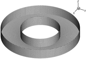
. Figure 3 shows one of the panellings used in WAMIT for
 $b=2\,a=$
20 m. In the WAMIT computations the floater is successively undergoing forced heave motion (to track the axisymmetric modes) then forced surge motion (for the antisymmetric modes). Response amplitude operators (RAOs) of the free surface elevation are obtained at selected locations in the moonpool. From peaks of the RAOs plotted versus the wave frequency, the resonant frequencies of the considered modes are derived. The frequency step is progressively refined around the peaks to increase accuracy.
Circular moonpool. Natural frequency of the piston mode for
 $a=10~\text{m}$
,
 $d=5~\text{m}$
,
 $b=30~\text{m}$
, and varying
 $c$
.

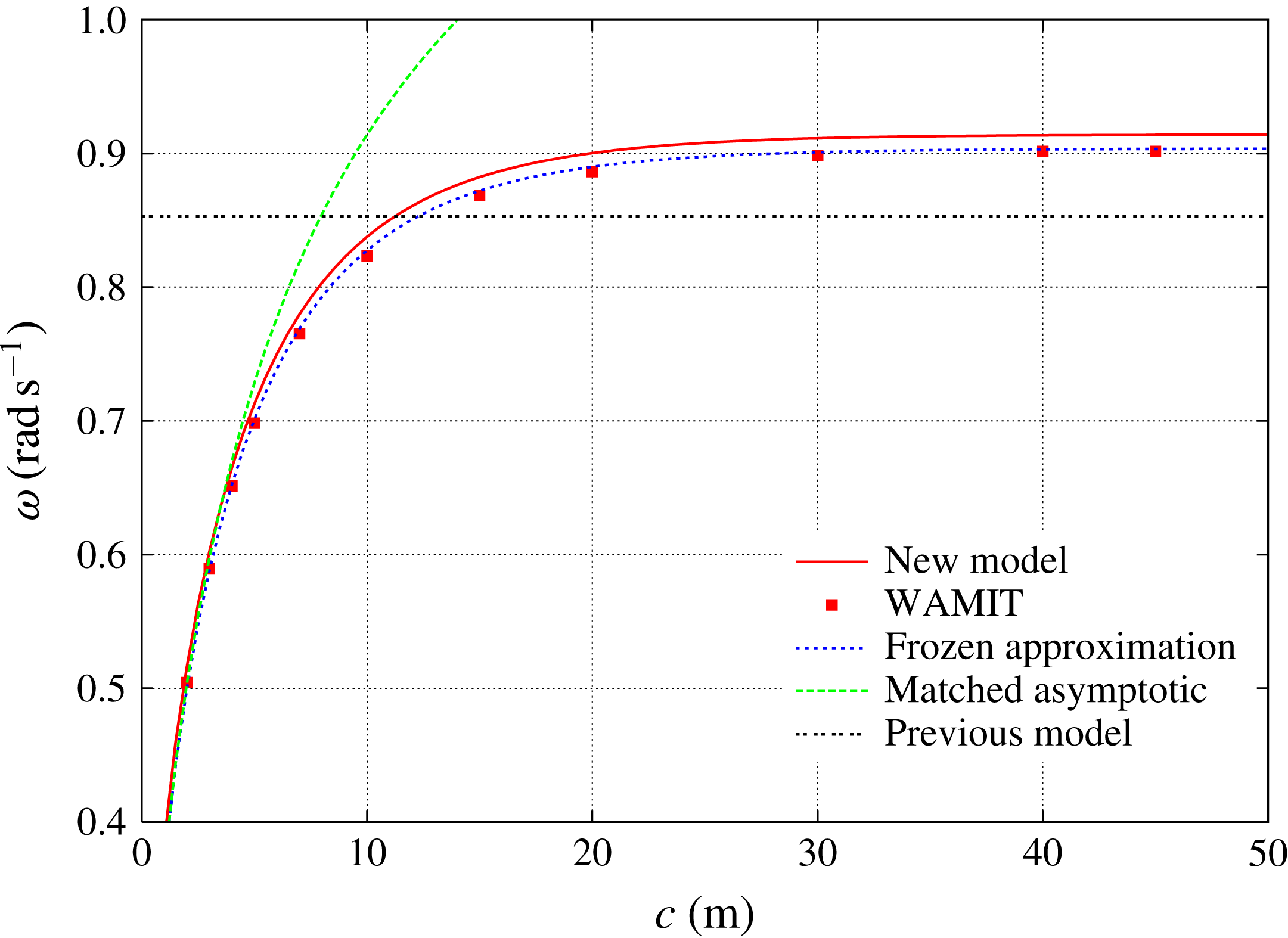
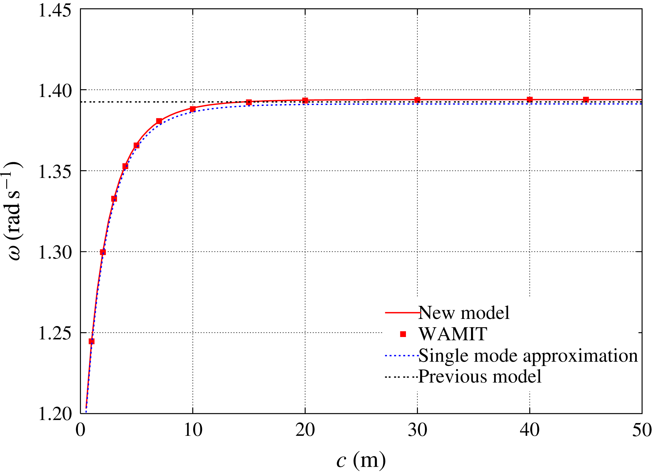
Figure 4 shows the obtained natural frequency of the piston mode when the outer radius is kept equal to 30 m and the clearance
 $c$
below the circular barge varies from a few metres up to 50 m. The values delivered by the new model are shown as a solid line, while the WAMIT values are shown as square symbols. The frequencies predicted with the frozen moonpool approximations (2.32) and (2.34) are also shown, together with the value given with the original model that assumes infinite depth and infinite outer radius. It can be seen that the values given by the new model, by the frozen moonpool approximation and by WAMIT are in good agreement. It is a bit striking that the WAMIT values agree better with the frozen moonpool approximation (2.32) than with the ‘exact’ calculations, but the differences are minor.
Circular moonpool. Natural frequency of the piston mode for
 $a=10~\text{m}$
,
 $d=5~\text{m}$
,
 $c=30~\text{m}$
, and varying
 $b/a$
.

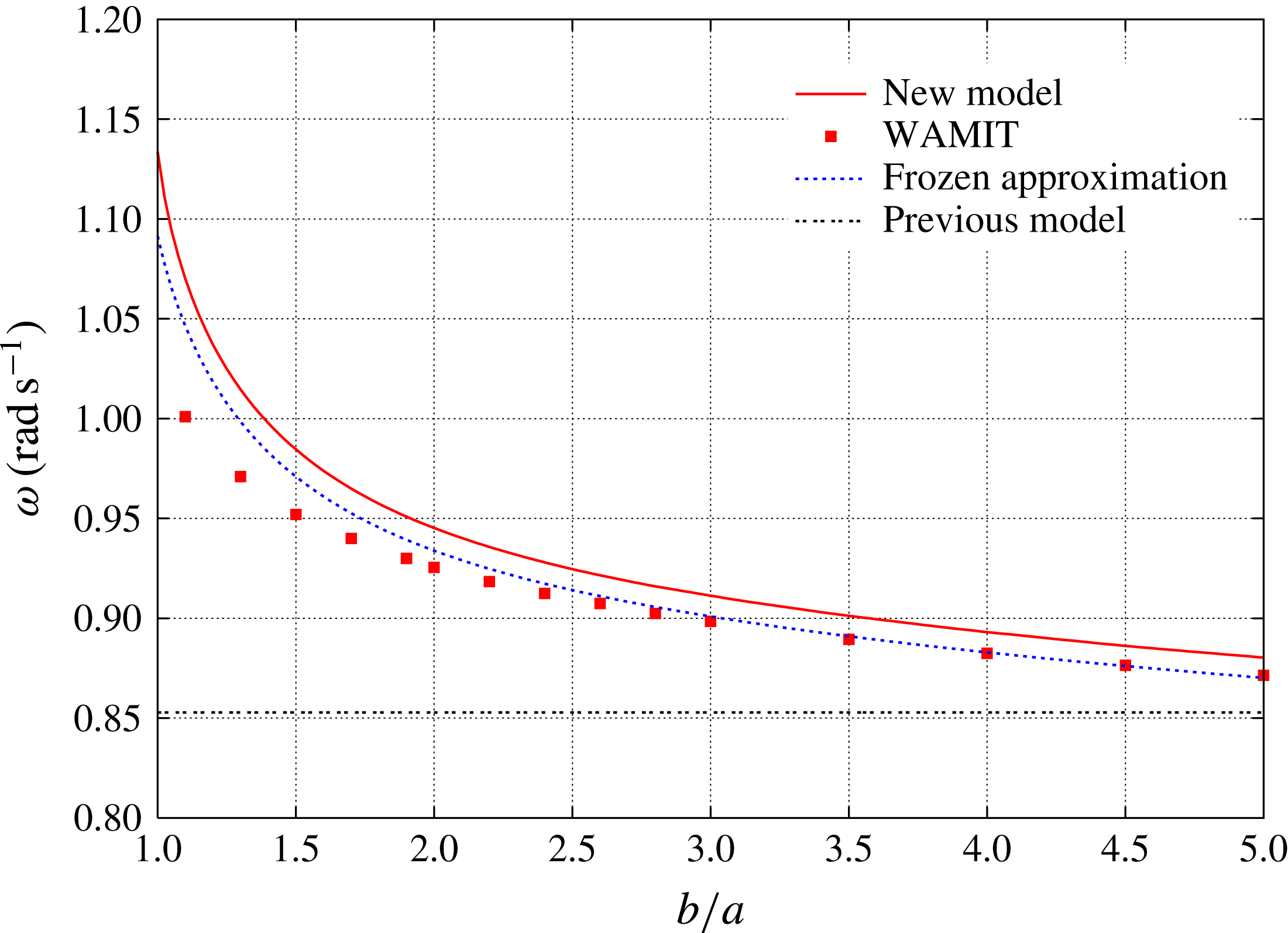
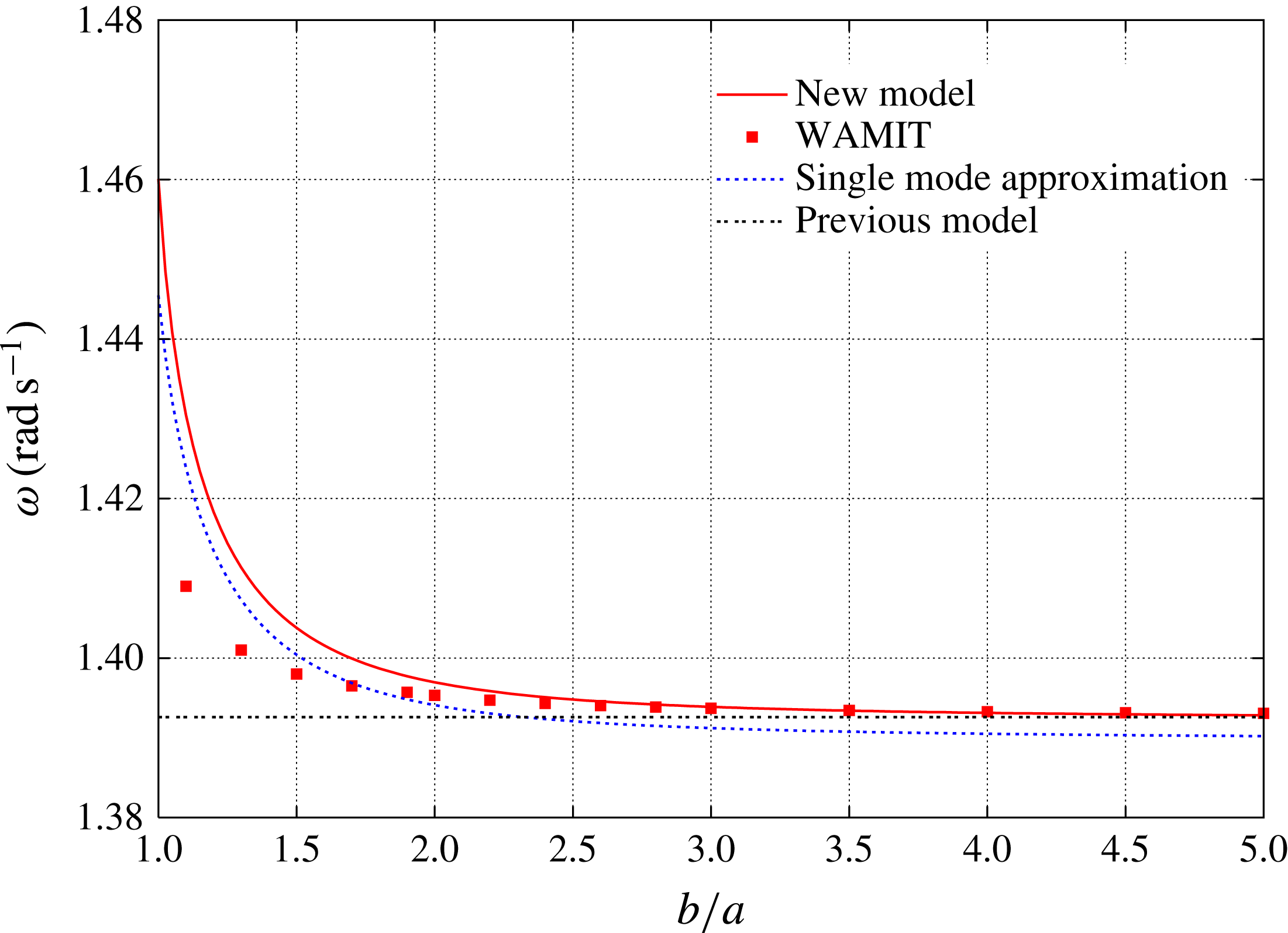
In figure 5 the clearance
 $c$
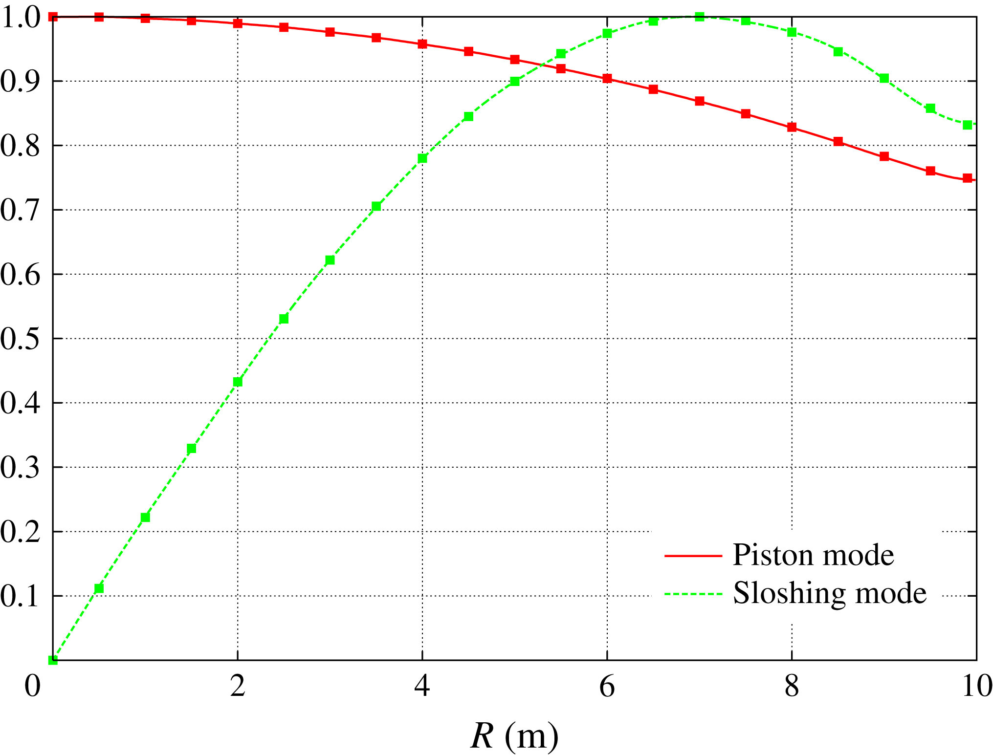
is kept equal to 30 m and the outer radius varies from 10 m up to 50 m. As compared with figure 4 it is to be noted that the frequency range is much reduced. Again the agreement between the natural frequencies delivered by WAMIT, by the new model and by the frozen moonpool approximation (2.32) are in good agreement and, again, the frozen approximation seems to be doing a better job. As the outer radius decreases, as could be expected, the agreement deteriorates somewhat. It looks like the outer radius
 $b$
should be taken somewhat larger than the actual value to ensure a good fit.
Circular moonpool. Natural frequency of the first antisymmetric sloshing mode for
 $a=10~\text{m}$
,
 $d=5~\text{m}$
,
 $b=30~\text{m}$
, and varying
 $c$
.

Circular moonpool. Natural frequency of the first antisymmetric sloshing mode for
 $a=10~\text{m}$
,
 $d=5~\text{m}$
,
 $c=30~\text{m}$
, and varying
 $b/a$
.

Figures 6 and 7 show analogous results in the case of the first antisymmetric sloshing mode. Again the natural frequencies given by WAMIT, by the new model and by the single-mode approximation (2.41) are in good agreement. Note, from figure 7, that there is very little sensitivity to the outer radius
 $b$
.
Circular moonpool. Modal shape of the piston mode for
 $a=10~\text{m}$
,
 $d=0.443~\text{m}$
.

Finally we show some modal shapes of the free surface, along a radius
 $0\leqslant R\leqslant a$
. For the piston mode, in order to observe significant deviations from a purely flat free surface, the draft
 $d$
of the moonpool needs to be substantially reduced. Here we take a draft
 $d$
equal to
 $\sqrt{S}/40$
, where
 $S=\unicode[STIX]{x03C0}\,a^{2}$
is the moonpool area. The same
 $\sqrt{S}/d$
ratio was considered in Molin (Reference Molin2001) in the square moonpool case (see figure 10 in that paper). So keeping the radius
 $a$
to 10 m we take a draft
 $d$
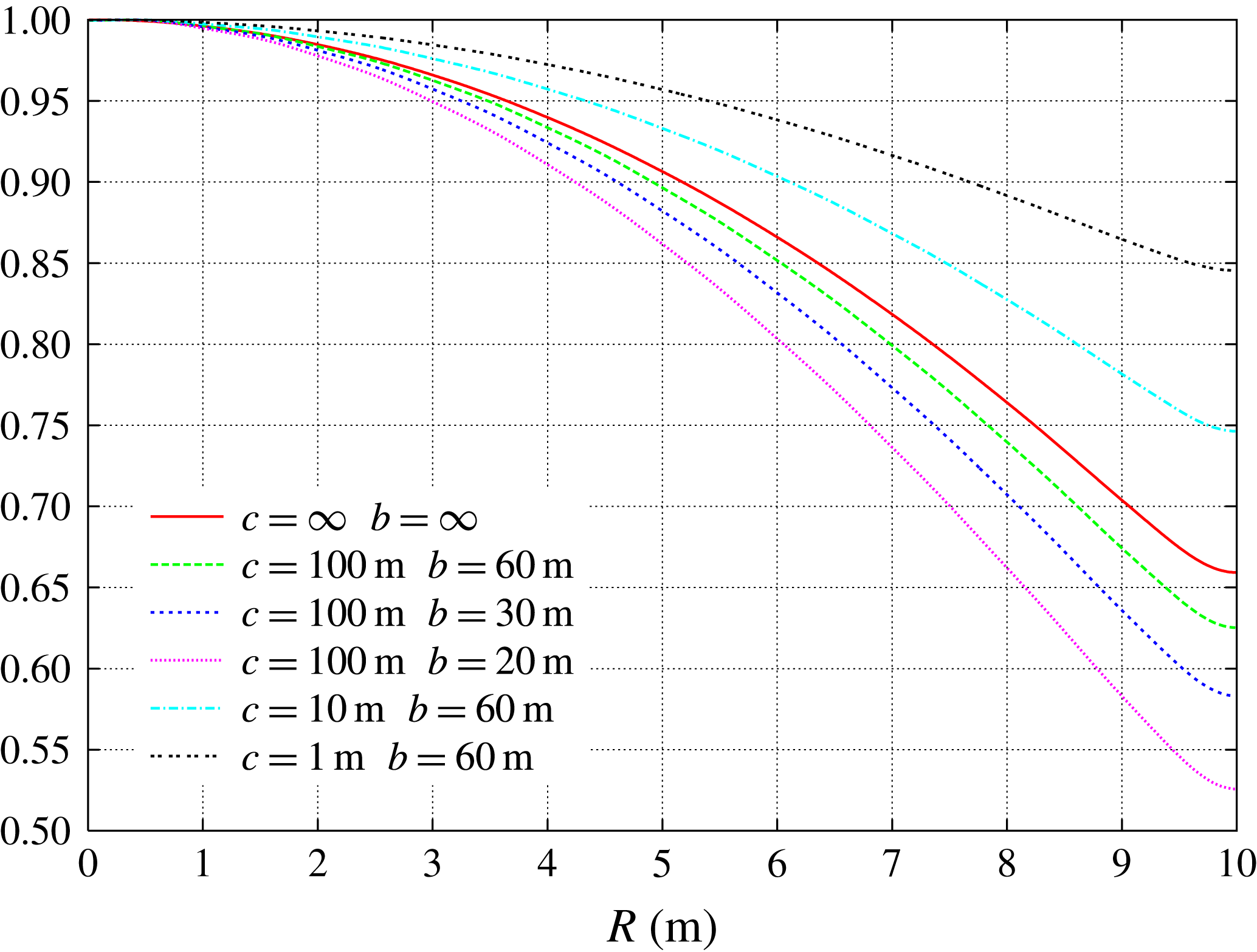
equal to 0.443 m. Figure 8 shows radial cuts of the free surface modal shape for different
 $c$
and
 $b$
values. The infinite depth/infinite radius case, from § 2.1, is also shown. Taking this case as a reference, it can be seen that, when the water height
 $c$
is being kept quasi-infinite (
 $c=100~\text{m}$
), the free surface gets lower and lower at the outer wall as the width
 $b$
is reduced. Conversely, when
 $b$
is kept constant (
 $b=30~\text{m}$
), the free surface profile becomes flatter and flatter as the clearance
 $c$
is reduced.
Circular moonpool. Modal shape of the first antisymmetric sloshing mode for
 $a=10~\text{m}$
.

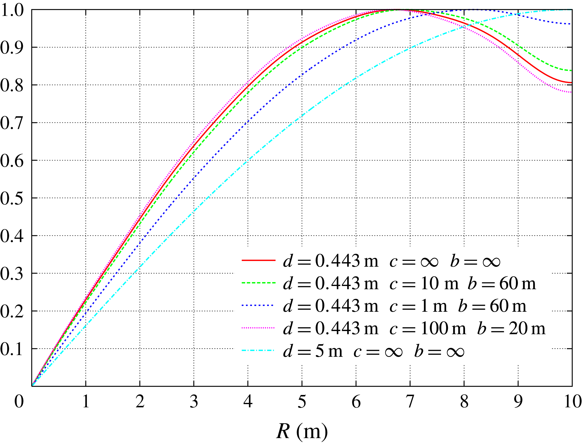
Figure 9 shows the modal shapes obtained for the first antisymmetric sloshing mode, for
 $0\leqslant R\leqslant a$
and
 $\unicode[STIX]{x1D703}=0$
. The same shallow draft (0.443 m) is considered but a deeper draft (5 m) is included for reference. In the deep draft case, the maximum elevation is obtained at the moonpool wall and the free surface shape closely follows the Bessel function
 $\text{J}_{1}(\unicode[STIX]{x1D707}_{1}R)$
. As the draft is reduced to 0.443 m the point of maximum elevation migrates away from the wall (a similar behaviour was observed in Molin (Reference Molin2001), for the first longitudinal sloshing mode, see figure 11 therein). As in the piston mode case, deviations from the infinite width and depth case increase when the outer radius decreases and decrease when the clearance decreases.
Circular moonpool. Modal shapes from our new model (lines) and from WAMIT (square symbols) for
 $d=0.443~\text{m}$
,
 $b=60~\text{m}$
and
 $c=10~\text{m}$
.

Finally, in figure 10, we show the modal shapes of the piston mode and of the first antisymmetric mode, from WAMIT and from our new model, in the case
 $d=0.443~\text{m}$
,
 $b=60~\text{m}$
and
 $c=10~\text{m}$
. It can be seen that the agreement is excellent.
3 Rectangular moonpool and gap in finite depth
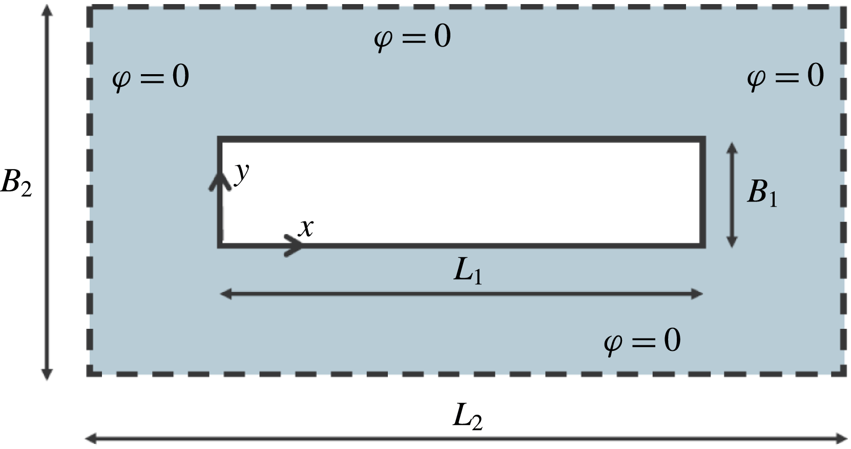
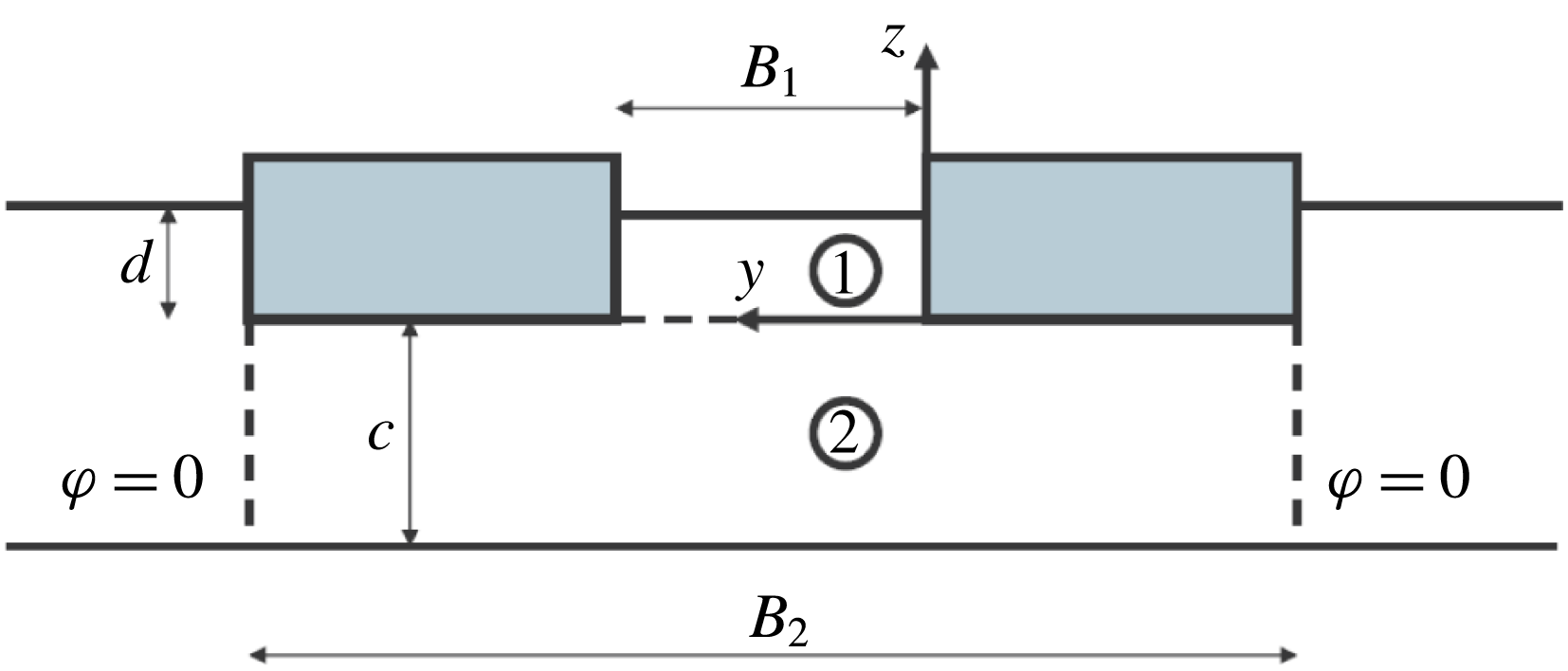
In this section we address the cases of a rectangular moonpool, inside a rectangular barge, and of two rectangular barges side by side. As illustrated in figures 11 and 12, the geometry is approximately the same in both cases. Mathematically the difference is that, in the moonpool case, an homogeneous Neumann condition is applied at the moonpool ends, whereas, in the gap case, an homogeneous Dirichlet condition is enforced. This simple end condition was first proposed by Newman & Sclavounos (Reference Newman and Sclavounos1988) and found to yield quite good approximations to the resonant frequencies in the gap.
Rectangular moonpool/gap. Geometry (from above).

Rectangular moonpool/gap. Geometry (transverse cut).

Figure 11 is a view from above that shows, with a full contour, the moonpool (or gap), and, in dashed contour, the outer boundary where we state the velocity potential to be nil. Laterally the position of this boundary would correspond to the outer edges of the barge(s).
Figure 12 is a transverse cut that shows the two hulls and the moonpool (or gap), and the lower fluid domain.
The coordinate system is located at one of the lower corners of the moonpool (or gap). The water height in the moonpool (the draft) is
 $d$
, the water height below the hulls (the clearance) is
 $c$
. The length of the moonpool is
 $L_{1}$
, its width is
 $B_{1}$
. The width of the lower domain is
 $B_{2}$
, its length is
 $L_{2}$
.
3.1 Gap
In the introduction we have argued that it is in the gap case that restricted water depths can be encountered. So we start with the gap case. Since gaps are usually very narrow we make the simplifying assumption that the flow within the gap is two-dimensional, i.e. the velocity potential
 $\unicode[STIX]{x1D711}_{1}$
only depends on the
 $x$
and
 $z$
coordinates. In § 3.3, devoted to the moonpool case, we relax this assumption.
Eigenfunction expansions
The velocity potential in the gap is written as
 $$\begin{eqnarray}\displaystyle & \displaystyle \unicode[STIX]{x1D711}_{1}(x,y,z)=\mathop{\sum }_{n=1}^{\infty }(A_{n}\,\cosh k_{n}z+B_{n}\,\sinh k_{n}z)\;\sin k_{n}x, & \displaystyle\end{eqnarray}$$
with
 $k_{n}=n\,\unicode[STIX]{x03C0}/L_{1}$
.
In the lower fluid domain it is a double series:
 $$\begin{eqnarray}\displaystyle & \displaystyle \unicode[STIX]{x1D711}_{2}(x,y,z)=\mathop{\sum }_{p=1}^{\infty }\mathop{\sum }_{q=1}^{\infty }C_{pq}\,\frac{\cosh \unicode[STIX]{x1D708}_{pq}(z+c)}{\cosh \unicode[STIX]{x1D708}_{pq}c}\;\sin \unicode[STIX]{x1D706}_{p}(x+a)\;\sin \unicode[STIX]{x1D707}_{q}(y+b), & \displaystyle\end{eqnarray}$$
with
 $$\begin{eqnarray}\displaystyle & \displaystyle \unicode[STIX]{x1D706}_{p}=p\,\unicode[STIX]{x03C0}/L_{2},\quad \unicode[STIX]{x1D707}_{q}=q\,\unicode[STIX]{x03C0}/B_{2},\quad \unicode[STIX]{x1D708}_{pq}^{2}=\unicode[STIX]{x1D706}_{p}^{2}+\unicode[STIX]{x1D707}_{q}^{2}, & \displaystyle\end{eqnarray}$$
 $p$
and
 $q$
integers, and
 $a=(L_{2}-L_{1})/2$
,
 $b=(B_{2}-B_{1})/2$
.
With these expansions the Laplace equation and the boundary conditions at the vertical boundaries (and at the seafloor) are fulfilled. It remains to match
 $\unicode[STIX]{x1D711}_{1}$
and
 $\unicode[STIX]{x1D711}_{2}$
on the boundary between subdomains 1 and 2, and match their vertical derivatives, and ensure that
 $\unicode[STIX]{x2202}\unicode[STIX]{x1D711}_{2}/\unicode[STIX]{x2202}z$
is zero below the two hulls. Again we use Garrett’s method (Garrett Reference Garrett1971).
Matching of the potentials
We must ensure
 $$\begin{eqnarray}\displaystyle & \displaystyle \mathop{\sum }_{n=1}^{N_{1}}A_{n}\,\sin k_{n}x=\mathop{\sum }_{p=1}^{N_{2x}}\mathop{\sum }_{q=1}^{N_{2y}}C_{pq}\,\sin \unicode[STIX]{x1D706}_{p}(x+a)\;\sin \unicode[STIX]{x1D707}_{q}(y+b), & \displaystyle\end{eqnarray}$$
for
 $0\leqslant x\leqslant L_{1}\;\;\;0\leqslant y\leqslant B_{1}$
.
Multiplying both sides with
 $\sin k_{m}x$
and integrating in
 $x$
and
 $y$
over the gap, we get, for each
 $m$
,
 $$\begin{eqnarray}\displaystyle & \displaystyle \frac{B_{1}\,L_{1}}{2}\,A_{m}=\mathop{\sum }_{p=1}^{N_{2x}}\mathop{\sum }_{q=1}^{N_{2y}}C_{pq}\;\int _{0}^{L_{1}}\sin \unicode[STIX]{x1D706}_{p}(x+a)\sin k_{m}x\;\text{d}x\;\int _{0}^{B_{1}}\sin \unicode[STIX]{x1D707}_{q}(y+b)\;\text{d}y, & \displaystyle\end{eqnarray}$$
or, in matrix form,
 $$\begin{eqnarray}\displaystyle & \displaystyle \boldsymbol{A}=\unicode[STIX]{x1D63C}\unicode[STIX]{x1D63E}\boldsymbol{\cdot }\boldsymbol{C}, & \displaystyle\end{eqnarray}$$
with
 $$\begin{eqnarray}\displaystyle \boldsymbol{A}=(A_{1},\ldots ,A_{N_{1}}),\quad \boldsymbol{C}=(C_{11},C_{12},\ldots ,C_{1N_{2y}},C_{21},\ldots ). & & \displaystyle\end{eqnarray}$$
The series have been truncated to order
 $N_{1}$
for
 $\unicode[STIX]{x1D711}_{1}$
and orders
 $N_{2x}$
,
 $N_{2y}$
for
 $\unicode[STIX]{x1D711}_{2}$
.
Vertical velocities
We must ensure
 $$\begin{eqnarray}\displaystyle \displaystyle \unicode[STIX]{x1D711}_{2z} & = & \displaystyle \unicode[STIX]{x1D711}_{1z},\quad 0\leqslant x\leqslant L_{1},\;0\leqslant y\leqslant B_{1}\nonumber\\ \displaystyle & = & \displaystyle 0,\quad \text{elsewhere}.\end{eqnarray}$$
That is
 $$\begin{eqnarray}\displaystyle & & \displaystyle \mathop{\sum }_{p}\mathop{\sum }_{q}\unicode[STIX]{x1D708}_{pq}\,C_{pq}\,\tanh \unicode[STIX]{x1D708}_{pq}\;\sin \unicode[STIX]{x1D706}_{p}(x+a)\;\sin \unicode[STIX]{x1D707}_{q}(y+b)=\mathop{\sum }_{n}k_{n}\,B_{n}\,\sin k_{n}x\nonumber\\ \displaystyle & & \displaystyle \qquad \text{for }0\leqslant x\leqslant L_{1}\,\,0\leqslant y\leqslant B_{1}\nonumber\\ \displaystyle & & \displaystyle \quad =0,\quad \text{elsewhere}.\end{eqnarray}$$
Multiplying both sides with
 $\sin \unicode[STIX]{x1D706}_{P}(x+a)\;\sin \unicode[STIX]{x1D707}_{Q}(y+b)$
and integrating over their domains of validity, we get, for each couple
 $(P,Q)$
:
 $$\begin{eqnarray}\displaystyle \frac{B_{2}L_{2}}{4}\unicode[STIX]{x1D708}_{PQ}C_{PQ}\tanh \unicode[STIX]{x1D708}_{PQ}=\mathop{\sum }_{n}k_{n}B_{n}\int _{0}^{L_{1}}\sin \unicode[STIX]{x1D706}_{P}(x+a)\sin k_{n}x\,\text{d}x\int _{0}^{B_{1}}\sin \unicode[STIX]{x1D707}_{Q}(y+b)\,\text{d}y, & & \displaystyle \nonumber\\ \displaystyle & & \displaystyle\end{eqnarray}$$
or, in matrix form:
 $$\begin{eqnarray}\displaystyle & \displaystyle \boldsymbol{C}=\unicode[STIX]{x1D63E}\unicode[STIX]{x1D63D}\boldsymbol{\cdot }\boldsymbol{B}. & \displaystyle\end{eqnarray}$$
 $$\begin{eqnarray}\displaystyle & \displaystyle \boldsymbol{A}=\unicode[STIX]{x1D63C}\unicode[STIX]{x1D63E}\boldsymbol{\cdot }\unicode[STIX]{x1D63E}\unicode[STIX]{x1D63D}\boldsymbol{\cdot }\boldsymbol{B}=\unicode[STIX]{x1D63C}\unicode[STIX]{x1D63D}\boldsymbol{\cdot }\boldsymbol{B}. & \displaystyle\end{eqnarray}$$
The following steps are identical to the cases considered before.
Single-mode approximations
Again single-mode approximations can be derived, when only one term is retained in (3.1). We obtain
 $$\begin{eqnarray}\displaystyle & \displaystyle \unicode[STIX]{x1D714}_{n}^{2}\simeq g\,k_{n}\;\frac{1+C_{n}\,\tanh k_{n}d}{\tanh k_{n}d+C_{n}}, & \displaystyle\end{eqnarray}$$
with
 $$\begin{eqnarray}\displaystyle & \displaystyle C_{n}=\frac{8\,k_{n}}{B_{1}\,L_{1}\,B_{2}\,L_{2}}\mathop{\sum }_{p=1}^{\infty }\mathop{\sum }_{q=1}^{\infty }\frac{K_{pn}^{2}\,\text{J}_{q}^{2}}{\unicode[STIX]{x1D708}_{pq}\;\tanh \unicode[STIX]{x1D708}_{pq}c}, & \displaystyle\end{eqnarray}$$
where
 $$\begin{eqnarray}\displaystyle & \displaystyle K_{pn}=\int _{0}^{L_{1}}\sin \unicode[STIX]{x1D706}_{p}(x+a)\;\sin k_{n}x\;\text{d}x,\quad \text{J}_{q}=\int _{0}^{B_{1}}\sin \unicode[STIX]{x1D707}_{q}(y+b)\;\text{d}y. & \displaystyle\end{eqnarray}$$
3.2 Comparison with resonant frequencies from Molin et al. (Reference Molin, Remy, Camhi and Ledoux2009)
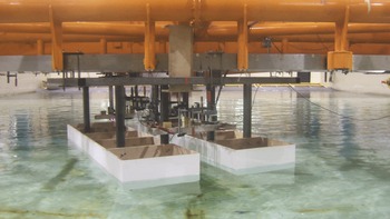
In Molin et al. (Reference Molin, Remy, Camhi and Ledoux2009) experimental and numerical results are reported for two identical rectangular barges side by side. The experiments took place in the offshore wave-tank BGO-FIRST located in la Seyne-sur-mer, near Toulon. This tank is 40 m long and 16 m wide. The water depth was set at 3 m during the tests. The barges were rigidly linked to the carriage, as shown in figure 13. The barge models had a length of 2.47 m, a width of 0.60 m and a draft of 0.18 m. The bilges were successively square then rounded, with a radius of curvature equal to 4 cm. Two gap widths were modelled: 12 and 31 cm. Here we only consider the narrower gap case, with the square bilges. The instrumentation consisted in nine resistive wave gauges on the centreline of the gap. The tests were run in irregular sea-states with Pierson–Moskowitz spectra of peak periods 1 s and 1.5 s. From the time series of the free surface elevation at the different gauges experimental RAOs were derived through standard spectral analysis.
Barge models in the tank.

Gap. Calculated RAOs of the free surface elevation at gauge 2.
 $0^{\circ }$
heading.

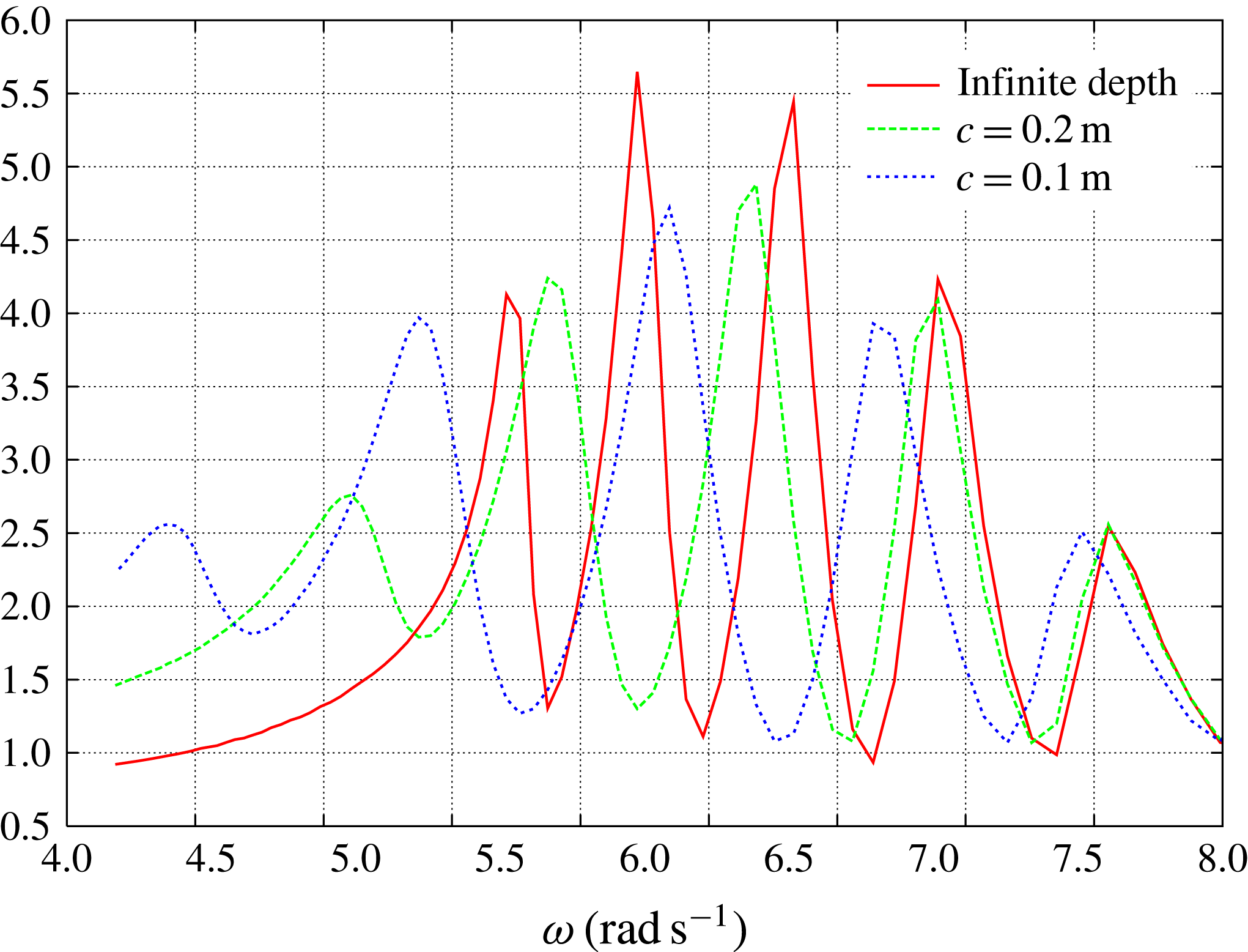
Computations were carried out with the software Diodore of Principia, analogous with WAMIT, and good agreement was found between the calculated peak frequencies of the RAOs and those derived from the experiments. Here we have repeated these calculations for water depths of 0.38 m, 0.28 m and 0.23 m – that is,
 $c$
values of 0.20 m, 0.10 m and 0.05 m. Figure 14 shows the calculated RAOs at the second gauge inside the gap (approximately 33.5 cm from the entrance), in head waves, for different values of the clearance (
 $c=0.05~\text{m}$
not shown). It can be seen that the peak frequencies shift to lower values as the clearance decreases.
Gap resonant frequencies (in
 $\text{rad}~\text{s}^{-1}$
) in large water depth.

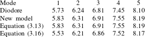
In table 3 we show the first five resonant frequencies obtained from Diodore and from the new model proposed here, in 3 m water depth. With the single-mode approximation formula (3.13) exactly the same values are obtained. Here the length
 $L_{2}$
of the lower subdomain has been taken equal to the barge length (
 $L_{2}=L_{1}=2.47~\text{m}$
) and its width
 $B_{2}$
has been taken equal to two times the barge width plus the gap width (
 $B_{2}=1.32~\text{m}$
).
In the last line are the resonant frequencies obtained by applying the formula that was proposed in Molin et al. (Reference Molin, Remy, Kimmoun and Stassen2002), based on Molin (Reference Molin2001), where the Neumann condition at the moonpool ends is replaced with an homogeneous Dirichlet condition. This formula, based on the single-mode approximation, can be written as
 $$\begin{eqnarray}\displaystyle \unicode[STIX]{x1D714}_{n}^{2}\simeq g\,\unicode[STIX]{x1D706}_{n}\;\frac{1+J_{n}\;\tanh \unicode[STIX]{x1D706}_{n}\,d}{J_{n}+\tanh \unicode[STIX]{x1D706}_{n}\,d}, & & \displaystyle\end{eqnarray}$$
where
 $$\begin{eqnarray}\displaystyle \displaystyle J_{n}(r) & = & \displaystyle \frac{2}{n\,\unicode[STIX]{x03C0}^{2}\,r}\left\{\int _{0}^{1}\frac{r^{2}}{u^{2}\;\sqrt{u^{2}+r^{2}}}\left[1+2u+(u-1)\cos (n\,\unicode[STIX]{x03C0}\,u)-\frac{3}{n\,\unicode[STIX]{x03C0}}\,\sin (n\,\unicode[STIX]{x03C0}\,u)\right]\text{d}u\right.\nonumber\\ \displaystyle & & \displaystyle \left.-\,\frac{1}{\sin \unicode[STIX]{x1D703}_{0}}+1+2r\,\ln \frac{1+\cos \unicode[STIX]{x1D703}_{0}}{1-\cos \unicode[STIX]{x1D703}_{0}}\right\},\end{eqnarray}$$
with
 $\unicode[STIX]{x1D706}_{n}=n\,\unicode[STIX]{x03C0}/L_{1}$
,
 $r=B_{1}/L_{1}$
and
 $\tan \unicode[STIX]{x1D703}_{0}=r^{-1}$
.
From table 3 it can be seen that the new model improves the prediction of the natural frequency of the first mode: the new model gives
 $5.83~\text{rad}~\text{s}^{-1}$
while Diodore gives
 $5.73~\text{rad}~\text{s}^{-1}$
and (3.16) gives
 $5.53~\text{rad}~\text{s}^{-1}$
. The first gap mode is analogous with the piston mode in the moonpool case since there is a net mass flux in the far field. Because of its infinite width assumption, (3.16) underestimates the natural frequency, while with the new model it seems to be overestimated. As already mentioned for the piston mode in the circular moonpool case, and as figure 15 suggests, better agreement would be obtained by slightly increasing the width of the barges in the new model. As for the following modes, the new model seems to perform less well than (3.16), but the differences are minor.
Gap. Variation of the natural frequencies of the first three modes with the width
 $(B_{2}-B_{1})/2$
of the barges.
 $L_{2}=L_{1}$
.

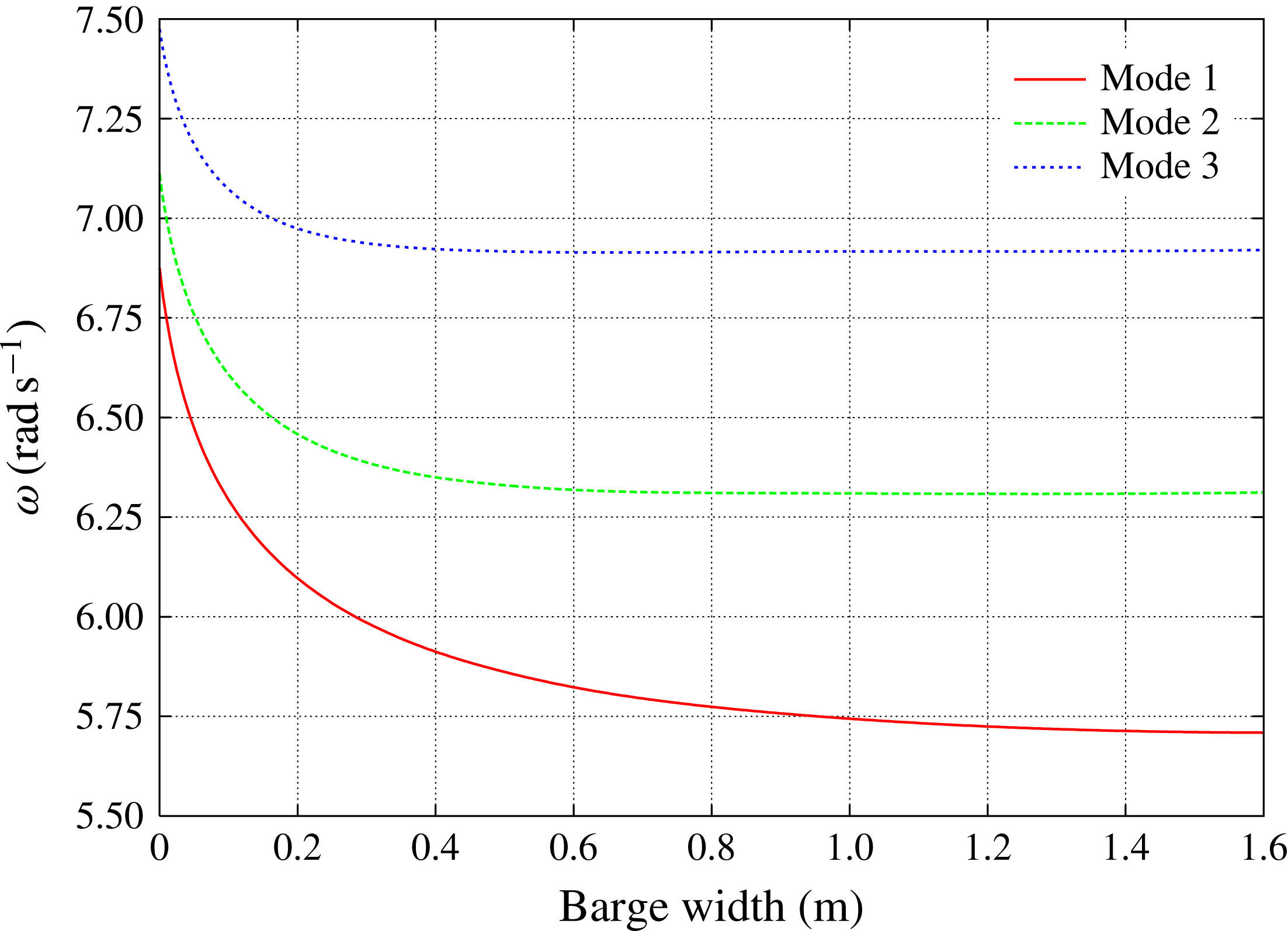
In figure 15 we vary the width
 $B_{2}$
of the lower domain, keeping its length
 $L_{2}$
equal to the gap length. As the equivalent barge width
 $(B_{2}-B_{1})/2$
increases the natural frequencies decrease. The values given in table 3 are for a width of 0.6 m. From the figure, as written above, it looks like a better prediction of the natural frequency of the first mode would be achieved by taking a width somewhat larger, between 0.8 m and 1 m. However, it would not improve much the prediction of the natural frequencies of the following modes.
Gap. Variation of the natural frequencies of the first three modes with the extra length
 $(L_{2}-L_{1})/2$
of the lower domain.
 $(B_{2}-B_{1})/2=1.6$
.

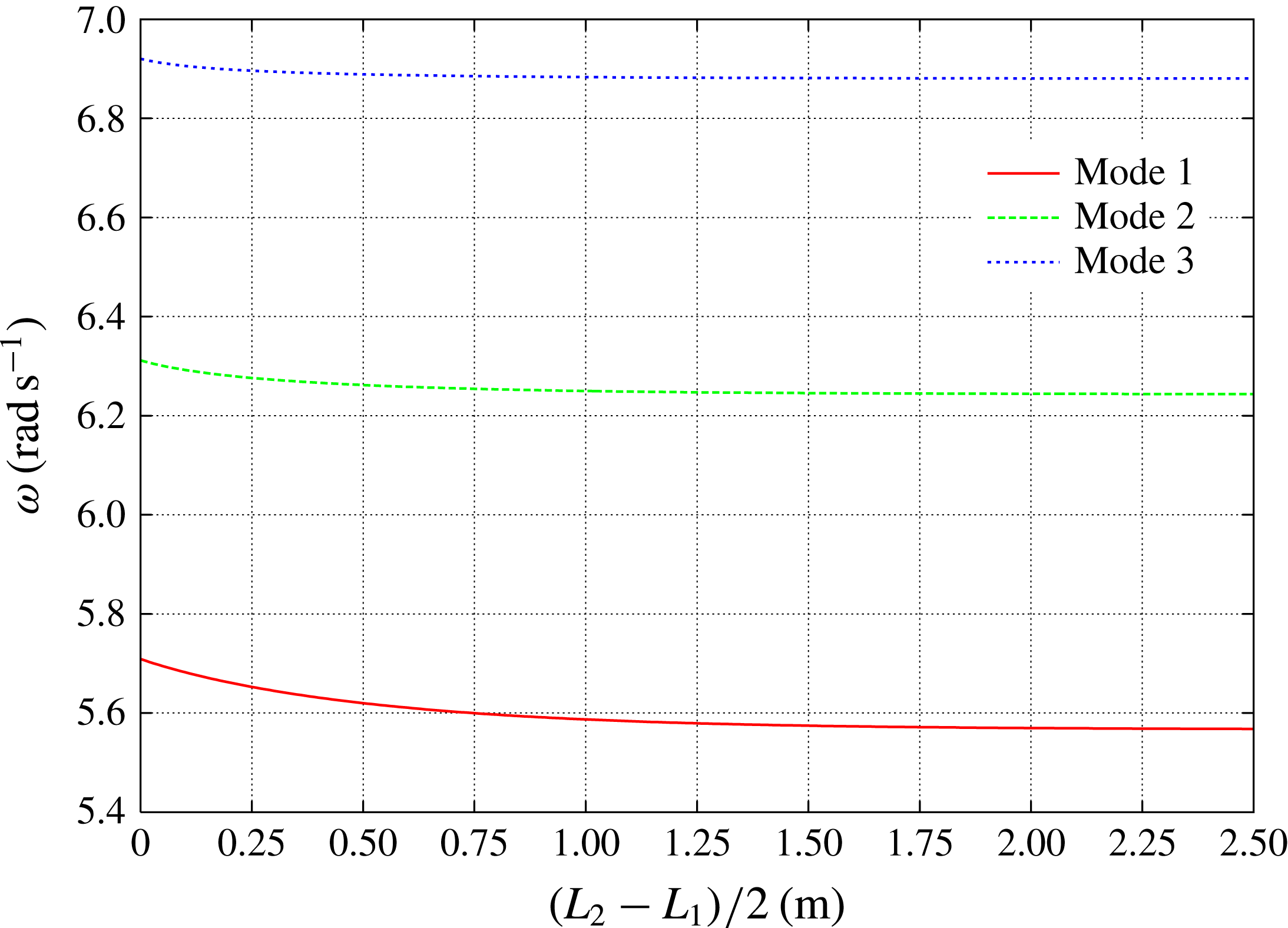
In figure 16 we keep the largest value of
 $(B_{2}-B_{1})/2$
from the previous calculations (1.6 m) and we vary the length
 $L_{2}$
of the lower domain. The natural frequencies decrease again and we get very close to the values given by (3.16) (approximately
 $5.56~\text{rad}~\text{s}^{-1}$
for
 $\unicode[STIX]{x1D714}_{1}$
when (3.16) gives
 $5.53~\text{rad}~\text{s}^{-1}$
, and even closer for the following modes).
Gap. Variation of the natural frequencies of the first three modes with the clearance
 $c$
below the barges.

In the results presented above, the water depth
 $h=c+d$
was taken equal to 3 m. Finally, in figure 17 we vary the water height
 $c$
below the barges, while keeping
 $(B_{2}-B_{1})/2=0.6~\text{m}$
and
 $L_{2}$
equal to the length of the barge. In the figure we plot, as square symbols, the natural frequencies derived from Diodore calculations at
 $c=2.82~\text{m}$
,
 $c=0.20~\text{m}$
,
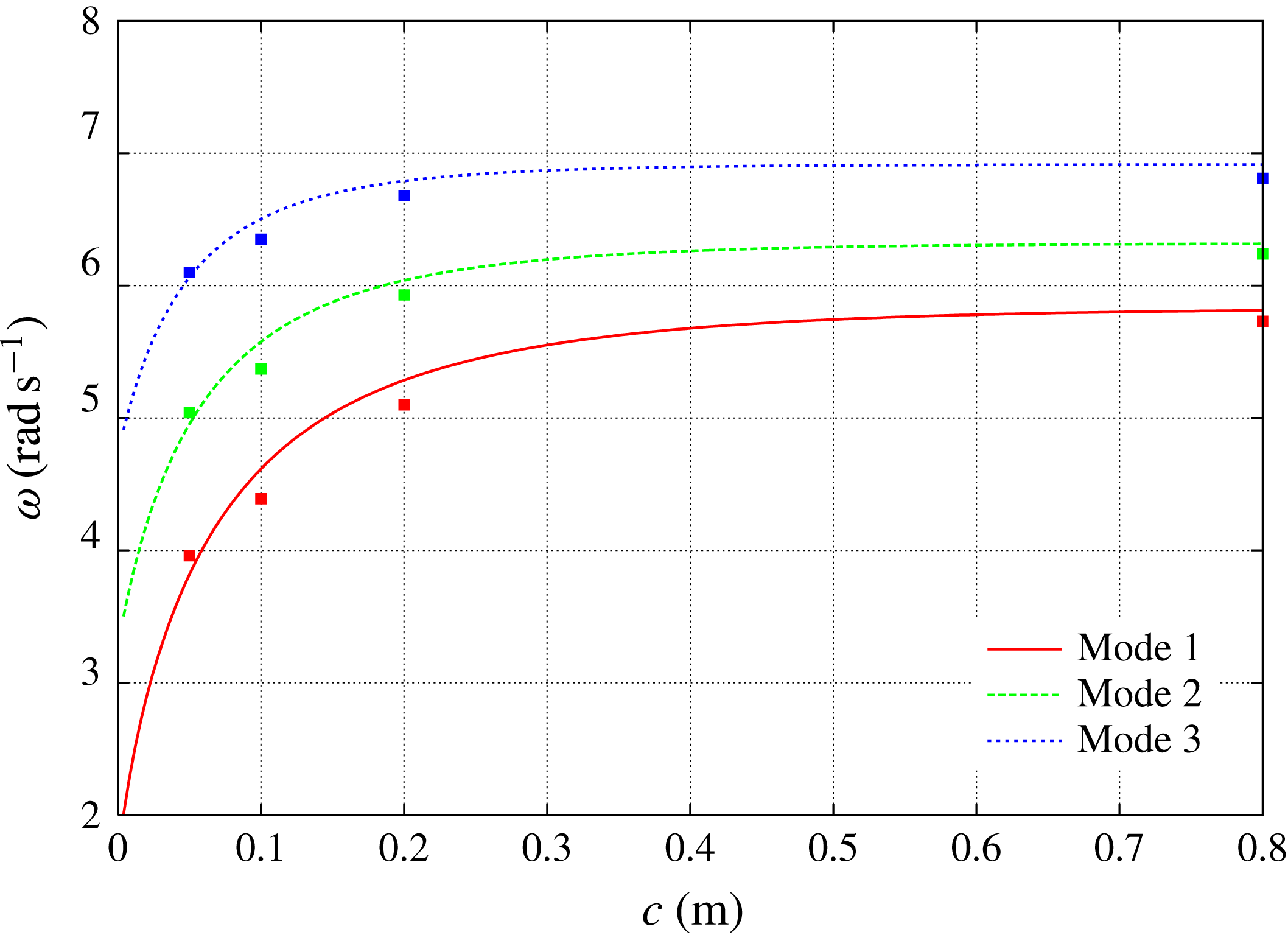
 $c=0.10~\text{m}$
and
 $c=0.05~\text{m}$
(see figure 14). For better clarity the
 $c=2.82~\text{m}$
values are shown at
 $c=0.8~\text{m}$
(the differences between 2.82 m and 0.8 m are minor). Overall the agreement between the values provided by the new model (or (3.13)) and by Diodore is rather good.
3.3 Moonpool
We assume the flow in the moonpool to be three-dimensional (in order to tackle the case of moonpools of large widths). The velocity potential in sub-domain 1 (the moonpool) is taken as
 $$\begin{eqnarray}\displaystyle \unicode[STIX]{x1D711}_{1}(x,y,z) & = & \displaystyle A_{00}+B_{00}\frac{z}{d}+\mathop{\sum }_{m=0}^{\infty }\mathop{\sum }_{\stackrel{n=0}{(m,n)\neq (0,0)}}^{\infty }\nonumber\\ \displaystyle & & \displaystyle \times \,[A_{mn}\cosh \unicode[STIX]{x1D708}_{mn}z+B_{mn}\sinh \unicode[STIX]{x1D708}_{mn}z]\cos \unicode[STIX]{x1D706}_{m}x\cos \unicode[STIX]{x1D707}_{n}y,\end{eqnarray}$$
with
 $$\begin{eqnarray}\displaystyle & \displaystyle \unicode[STIX]{x1D706}_{m}=m\,\unicode[STIX]{x03C0}/L_{1},\quad \unicode[STIX]{x1D707}_{n}=n\,\unicode[STIX]{x03C0}/B_{1},\quad \unicode[STIX]{x1D708}_{mn}^{2}=\unicode[STIX]{x1D706}_{m}^{2}+\unicode[STIX]{x1D707}_{n}^{2}. & \displaystyle\end{eqnarray}$$
In the lower sub-domain it is the same as in the gap case (with different notations for the wave numbers):
 $$\begin{eqnarray}\displaystyle & \displaystyle \unicode[STIX]{x1D711}_{2}(x,y,z)=\mathop{\sum }_{p=1}^{\infty }\mathop{\sum }_{q=1}^{\infty }C_{pq}\,\frac{\cosh \unicode[STIX]{x1D6FE}_{pq}(z+c)}{\cosh \unicode[STIX]{x1D6FE}_{pq}c}\;\sin \unicode[STIX]{x1D6FC}_{p}(x+a)\;\sin \unicode[STIX]{x1D6FD}_{q}(y+b), & \displaystyle\end{eqnarray}$$
with
 $$\begin{eqnarray}\displaystyle & \displaystyle \unicode[STIX]{x1D6FC}_{p}=p\,\unicode[STIX]{x03C0}/L_{2},\quad \unicode[STIX]{x1D6FD}_{q}=q\,\unicode[STIX]{x03C0}/B_{2},\quad \unicode[STIX]{x1D6FE}_{pq}^{2}=\unicode[STIX]{x1D6FC}_{p}^{2}+\unicode[STIX]{x1D6FD}_{q}^{2}, & \displaystyle\end{eqnarray}$$
 $p$
and
 $q$
integers, and
 $a=(L_{2}-L_{1})/2$
,
 $b=(B_{2}-B_{1})/2$
.
The following procedure of matching the potentials, then their vertical derivatives, is identical to that of the gap case, so it is not repeated here.
Single-mode approximations
Single-mode approximations may again easily be derived. We get:
Piston mode:
 $$\begin{eqnarray}\displaystyle & \displaystyle \unicode[STIX]{x1D714}_{00}^{2}\simeq \frac{g}{d}\;\frac{1}{1+C_{00}}, & \displaystyle\end{eqnarray}$$
with
 $$\begin{eqnarray}\displaystyle & \displaystyle C_{00}=\frac{4}{B_{1}\,L_{1}\,B_{2}\,L_{2}\,d}\mathop{\sum }_{p=1}^{\infty }\mathop{\sum }_{q=1}^{\infty }\frac{I_{p}^{2}\,\text{J}_{q}^{2}}{\unicode[STIX]{x1D6FE}_{pq}\,\tanh \unicode[STIX]{x1D6FE}_{pq}c}, & \displaystyle\end{eqnarray}$$
and
 $$\begin{eqnarray}\displaystyle & \displaystyle I_{p}=\int _{0}^{L_{1}}\sin \unicode[STIX]{x1D6FC}_{p}(x+a)\;\text{d}x,\quad \text{J}_{q}=\int _{0}^{B_{1}}\sin \unicode[STIX]{x1D6FD}_{q}(y+b)\;\text{d}y. & \displaystyle\end{eqnarray}$$
Longitudinal sloshing modes:
 $$\begin{eqnarray}\displaystyle & \displaystyle \unicode[STIX]{x1D714}_{m0}^{2}\simeq g\,\unicode[STIX]{x1D706}_{m}\;\frac{1+C_{m0}\,\tanh \unicode[STIX]{x1D706}_{m}d}{\tanh \unicode[STIX]{x1D706}_{m}d+C_{m0}}, & \displaystyle\end{eqnarray}$$
with
 $$\begin{eqnarray}\displaystyle & \displaystyle C_{m0}=\frac{8\,\unicode[STIX]{x1D706}_{m}}{B_{1}\,L_{1}\,B_{2}\,L_{2}}\mathop{\sum }_{p=1}^{\infty }\mathop{\sum }_{q=1}^{\infty }\frac{K_{pm}^{2}\,\text{J}_{q}^{2}}{\unicode[STIX]{x1D6FE}_{pq}\,\tanh \unicode[STIX]{x1D6FE}_{pq}c}, & \displaystyle\end{eqnarray}$$
and
 $$\begin{eqnarray}\displaystyle & \displaystyle K_{pm}=\int _{0}^{L_{1}}\sin \unicode[STIX]{x1D6FC}_{p}(x+a)\;\cos \unicode[STIX]{x1D706}_{m}x\;\text{d}x,\quad \text{J}_{q}=\int _{0}^{B_{1}}\sin \unicode[STIX]{x1D6FD}_{q}(y+b)\;\text{d}y. & \displaystyle\end{eqnarray}$$
3.4 Applications
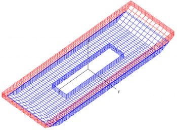
As written earlier, ships and offshore structures equipped with moonpools usually operate in deep water. So we will focus here on the sensitivity of the natural frequencies to the beam of the support. We take the case of the Wellhead Barge (WHB) developed by Saipem (for example, see Maisondieu & Le Boulluec Reference Maisondieu and Le Boulluec2001a ). Figure 18 shows the panelling of the WHB that was used for diffraction-radiation analysis with Diodore.
Wellhead Barge. Panelling for Diodore computations.

The barge is 180 m long and 60 m wide, the moonpool length is 80 m and its width 20 m, and the draft is 6.5 m. In the computations we take the length
 $L_{2}$
of the lower domain equal to 180 m (the barge length) and we vary its width
 $B_{2}$
. The clearance
 $c$
is taken as 300 m.
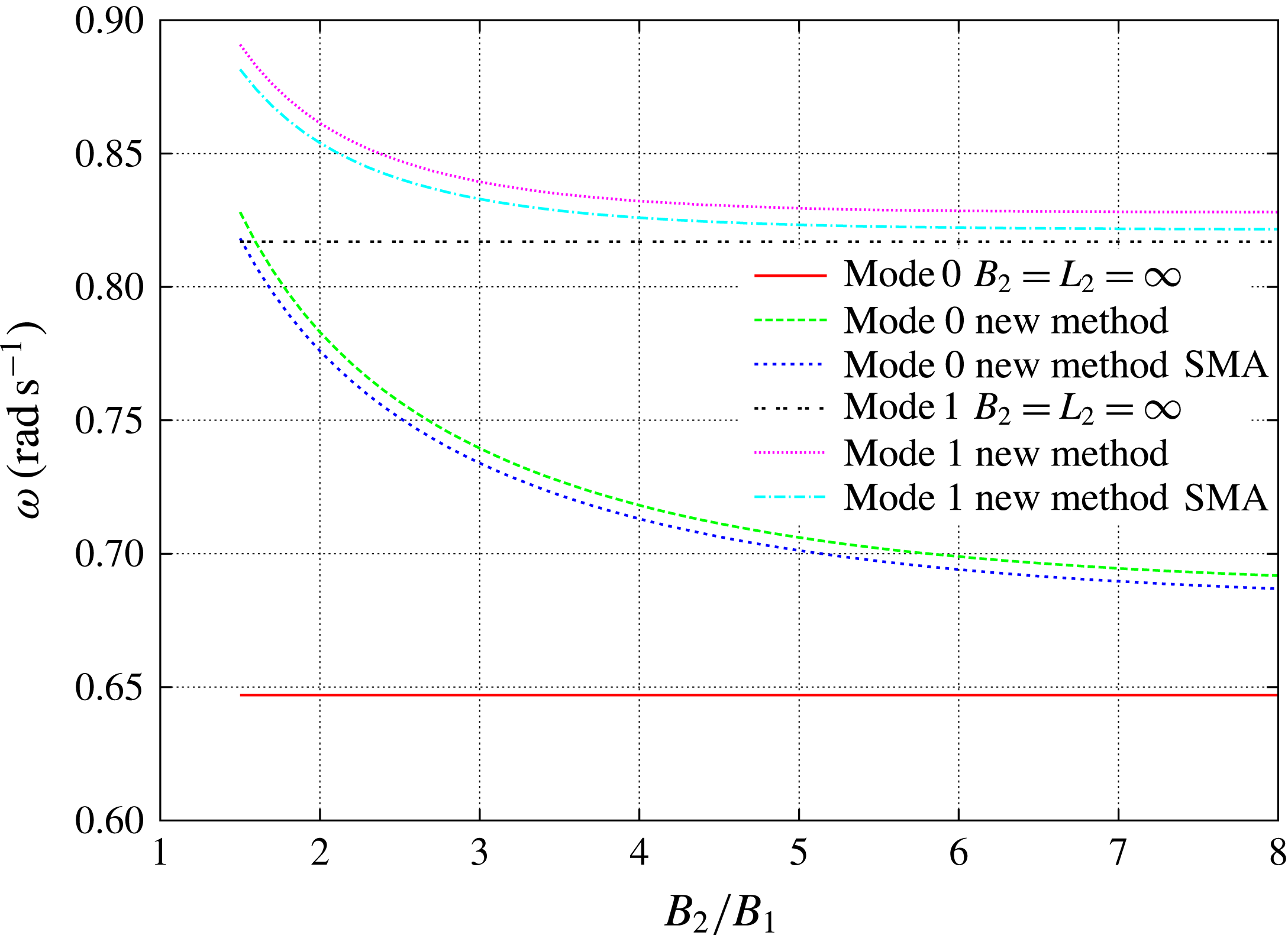
Wellhead Barge. Natural frequencies of the piston (mode 0) and first sloshing (mode 1) modes versus the width
 $B_{2}$
of the lower domain.

Figure 19 shows the frequencies obtained for the piston and first sloshing modes. For each mode, three curves are shown: the values given by the earlier method (Molin Reference Molin2001) that assumes infinite length and width (straight lines in the figure), the values given by the new method and by the single-mode approximation (3.22) or (3.25) given above. Diodore calculations give natural frequencies of
 $0.7~\text{rad}~\text{s}^{-1}$
for the piston mode and
 $0.84~\text{rad}~\text{s}^{-1}$
for the first sloshing mode. These values are taken from the locations of the peaks in the heave and surge radiation dampings. Taking as a reference position
 $B_{2}/B_{1}=3$
it can be seen that the Diodore value of the piston mode frequency is in-between the values delivered by the two methods. Or, in other terms, that the ratio
 $B_{2}/B_{1}$
used in applying the new method should be taken somewhat larger than the actual
 $B_{2}/B_{1}$
. This is consistent with the conclusions derived in the circular case. As for the first sloshing mode, as already observed, its natural frequency is only slightly sensitive to the barge width (due to zero mass flux in the far field), and a minor improvement is obtained in applying the new method.
As a second and final application, we consider a floating foundation for a wind turbine, with a large square moonpool, described in Guignier et al. (Reference Guignier, Courbois, Mariani and Choisnet2016). The moonpool is
 $27~\text{m}\times 27~\text{m}$
, while the outer hull is
 $45~\text{m}\times 45~\text{m}$
. It is fitted with additional bilge keels, 3 m wide (Guignier, personal communication), so we take a width and length of 51 m for the lower subdomain. The draft is 7 m and the water depth is 55 m.
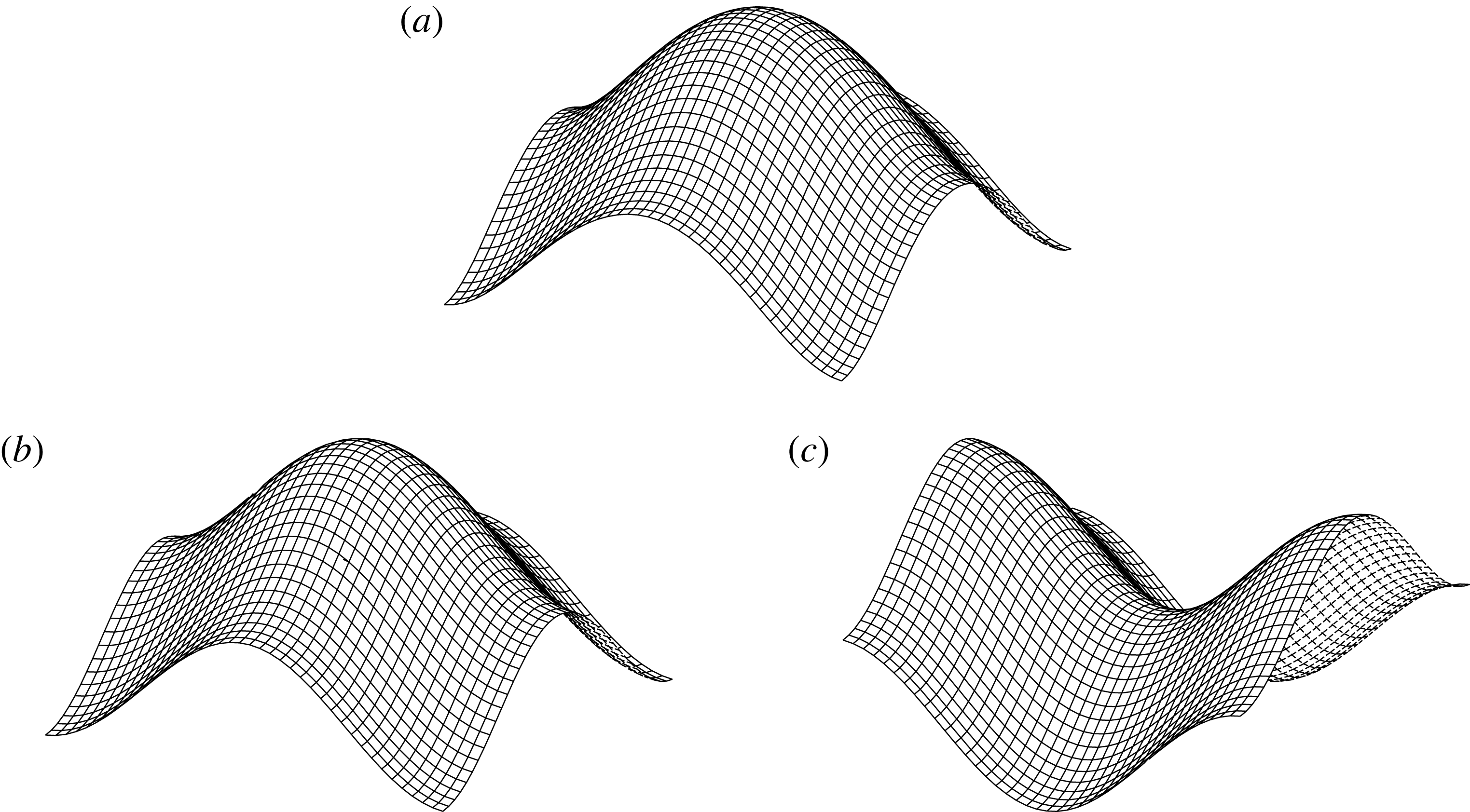
Square moonpool. Free surface shapes for mode 0 (a), mode 4 (b) and mode 5 (c).

Wind turbine floating foundation. Natural frequencies.

Table 4 gives the calculated frequencies of the first eight modes obtained. The estimated values, given in the second line, are from the single-mode approximations (3.22) and (3.25). From the peaks in the heave and surge radiation dampings calculated with the diffraction software Aqwa, the natural frequencies of the piston and first sloshing modes are, respectively,
 $0.78~\text{rad}~\text{s}^{-1}$
and
 $1.1~\text{rad}~\text{s}^{-1}$
(Guignier, personal communication), so the agreement with our values is rather good. With the former model of Molin (Reference Molin2001) the corresponding values are
 $0.704~\text{rad}~\text{s}^{-1}$
and
 $1.12~\text{rad}~\text{s}^{-1}$
.
The last line in table 4 gives the
 $(m,n)$
values of the dominant geometric modes (
 $\cos \unicode[STIX]{x1D706}_{m}x\;\cos \unicode[STIX]{x1D706}_{n}y$
) in the modal shapes of the free surface elevation. Mode 0 is the piston mode. Modes 1 and 2 are the first sloshing modes in the
 $x$
and
 $y$
directions, hence they have the same natural frequencies. Likewise for modes 6 and 7 which are identical. However, modes 4 and 5 are not a double mode; they are different and they have slightly different natural frequencies. They both have the geometric modes (2, 0) and (0, 2) contributing with equal amplitudes, but different signs: in mode 4 they add up, in mode 5 they subtract. In mode 4 the corners and the centre of the moonpool are antinodes, in mode 5 they are nodes. Both modes are shown in figure 20, together with mode 0. It can be seen that mode 4 looks very much like mode 0; however, the figure is somewhat misleading, as the vertical scales are different: for the piston mode (mode 0), the range is from 0.89 (in the corner) to 1 (in the centre), the free surface is nearly flat (due to the large draft) as it heaves up and down. For mode 4 the range is from
 $-1$
(in the corner) to
 $+1$
(in the centre). However, the geometric mode
 $(0,0)$
does participate to mode 4 (there is also a small contribution from mode (2, 2)), meaning that the mean water level heaves up and down, and that a net mass flux is associated. Mode 4 is very much like the first axisymmetric sloshing mode in the circular moonpool case (see paragraph 2.1.1). As for mode 5, only the geometric modes
 $(0,2)$
and
 $(2,0)$
participate, there is no variation in the mean free surface level.
This is very much unlike what happens in a rectangular tank (with a bottom), where each geometric mode of the form
 $\cos \unicode[STIX]{x1D706}_{m}x\;\cos \unicode[STIX]{x1D707}_{n}y$
is a natural mode. In the moonpool case, connection with the lower fluid domain creates coupling between the geometric modes.
4 Final comments
We have proposed a modification of the original theoretical model of Molin (Reference Molin2001) that permits one to derive the resonant modes of gaps and moonpools in finite depth. Another difference from Molin (Reference Molin2001) is that the new model accounts, to some extent, for the finite horizontal dimensions of the floating support. In the new model the lower subdomain, below the keel line, is now finite, bounded by the hull, by the seafloor and by an artificial vertical cylinder where the velocity potential is taken to be nil.
Applications have been made to circular and rectangular moonpools, and to narrow rectangular gaps. The obtained natural frequencies have been compared with numerical values derived from calculations with state-of-the-art diffraction-radiation codes (WAMIT 2016 and Diodore 0000). The new model has been found to correctly account for finite depth. As for accounting for the finite horizontal dimensions of the support, it appears that, when the outer artificial cylinder runs through the waterline of the support, the calculated resonant frequencies of the piston mode (or first sloshing mode in the gap case) are slightly overestimated. A similar situation occurred in the two-dimensional moonpool case in Molin (Reference Molin2001), where two sinks were located at either side at
 $\pm \unicode[STIX]{x1D706}\,B/2$
, with
 $B$
being the beam, and where it was found that the coefficient
 $\unicode[STIX]{x1D706}$
needed to be taken somewhat larger than unity for a good fit (Maisondieu et al.
Reference Maisondieu, Molin, Kimmoun and Gentaz2001b
; Faltinsen et al.
Reference Faltinsen, Rognebakke and Timokha2007). In very shallow water depth, improvements of the method could certainly be made, through matched asymptotic expansions, following, for example, the works of Newman, Sortland & Vinje (Reference Newman, Sortland and Vinje1984) or Molin et al. (Reference Molin, Guérin, Martigny and Weber1999). However, it might not be that easy in intermediate depth.
Simple expressions (single-mode approximations) have been proposed that give first estimates of the resonant frequencies. These formulas have more generality than those given in Molin (Reference Molin2001) and Molin et al. (Reference Molin, Remy, Kimmoun and Stassen2002) and they are easy to implement. It is believed that they can be helpful to offshore engineers.
Finally, as compared to Molin (Reference Molin2001), the proposed finite depth model is much easier to implement and much faster to run, allowing for easy variations of the geometric parameters.
Appendix A. Calculation of the matrix
$\unicode[STIX]{x1D63C}\unicode[STIX]{x1D63D}$

The bottom boundary condition (2.9) can be written as
 $$\begin{eqnarray}\displaystyle & \displaystyle A_{0}+\mathop{\sum }_{n}A_{n}\,\text{J}_{0}(k_{n}R)=\frac{1}{2\unicode[STIX]{x03C0}}\int _{0}^{a}r\,\text{d}r\,\int _{0}^{2\unicode[STIX]{x03C0}}\frac{B_{0}/d+\displaystyle \mathop{\sum }_{n}B_{n}k_{n}\,\text{J}_{0}(k_{n}r)}{\sqrt{R^{2}+r^{2}-2Rr\,\cos (\unicode[STIX]{x1D703}-\unicode[STIX]{x1D6FC})}}\;\text{d}\unicode[STIX]{x1D6FC}. & \displaystyle\end{eqnarray}$$
(1) Integrate each side over the disc:
 $$\begin{eqnarray}\displaystyle \left.\begin{array}{@{}l@{}}\displaystyle \unicode[STIX]{x03C0}\,a^{2}\,A_{0}=\frac{1}{2\unicode[STIX]{x03C0}}\int _{0}^{2\unicode[STIX]{x03C0}}\text{d}\unicode[STIX]{x1D703}\int _{0}^{a}R\,\text{d}R\int _{0}^{a}r\,\text{d}r\,\int _{0}^{2\unicode[STIX]{x03C0}}\frac{B_{0}/d+\displaystyle \mathop{\sum }_{n}B_{n}k_{n}\,\text{J}_{0}(k_{n}r)}{\sqrt{R^{2}+r^{2}-2Rr\,\cos (\unicode[STIX]{x1D703}-\unicode[STIX]{x1D6FC})}}\;\text{d}\unicode[STIX]{x1D6FC}\\ \displaystyle \unicode[STIX]{x03C0}\,a^{2}\,A_{0}=\int _{0}^{a}R\,\text{d}R\int _{0}^{a}r\,\text{d}r\,\int _{0}^{2\unicode[STIX]{x03C0}}\frac{B_{0}/d+\displaystyle \mathop{\sum }_{n}B_{n}k_{n}\,\text{J}_{0}(k_{n}r)}{\sqrt{R^{2}+r^{2}-2Rr\,\cos \unicode[STIX]{x1D6FD}}}\;\text{d}\unicode[STIX]{x1D6FD}\\ \displaystyle \unicode[STIX]{x03C0}\,a^{2}\,A_{0}=4\int _{0}^{a}R\,\text{d}R\int _{0}^{a}r\,\text{d}r\,\frac{1}{|R-r|}\,\left[B_{0}/d+\mathop{\sum }_{n}B_{n}k_{n}\,\text{J}_{0}(k_{n}r)\right]K\left(-\frac{4Rr}{(R-r)^{2}}\right)\\ \displaystyle \unicode[STIX]{x03C0}\,a^{2}\,A_{0}=\frac{8\,a^{3}}{3\,d}\,B_{0}+\mathop{\sum }_{n}k_{n}\,B_{n}\int _{0}^{a}\int _{0}^{a}\frac{R\,r}{|R-r|}\,K\left(-\frac{4Rr}{(R-r)^{2}}\right)\text{J}_{0}(k_{n}r)\,\text{d}R\;\text{d}r,\end{array}\right\} & & \displaystyle\end{eqnarray}$$
with
 $K$
the complete elliptic function of the first kind and, for negative argument:
 $$\begin{eqnarray}\displaystyle & \displaystyle K(-m)=\frac{1}{\sqrt{1+m}}\,K\left(\frac{m}{m+1}\right). & \displaystyle\end{eqnarray}$$
(2) Now multiply each side with
 $\text{J}_{0}(k_{m}R)$
and integrate over the disc:
 $$\begin{eqnarray}\displaystyle & & \displaystyle 2\,\unicode[STIX]{x03C0}\,A_{m}\,\int _{0}^{a}\text{J}_{0}^{2}(k_{m}R)\,R\,\text{d}R=\frac{1}{2\unicode[STIX]{x03C0}}\int _{0}^{2\unicode[STIX]{x03C0}}\text{d}\unicode[STIX]{x1D703}\int _{0}^{a}R\,\text{d}R\int _{0}^{a}r\,\text{d}r\,\nonumber\\ \displaystyle & & \displaystyle \quad \times \,\int _{0}^{2\unicode[STIX]{x03C0}}\frac{B_{0}/d+\displaystyle \mathop{\sum }_{n}B_{n}k_{n}\,\text{J}_{0}(k_{n}r)}{\sqrt{R^{2}+r^{2}-2Rr\,\cos (\unicode[STIX]{x1D703}-\unicode[STIX]{x1D6FC})}}\,\text{J}_{0}(k_{m}R)\;\text{d}\unicode[STIX]{x1D6FC}\nonumber\\ \displaystyle & & \displaystyle \quad \unicode[STIX]{x03C0}\,a^{2}\,\text{J}_{0}^{2}(k_{m}a)\,A_{m}=\frac{4\,B_{0}}{d}\int _{0}^{a}\int _{0}^{a}\frac{R\,r}{|R-r|}\,K\left(-\frac{4Rr}{(R-r)^{2}}\right)\,\text{J}_{0}(k_{m}R)\,\text{d}R\;\text{d}r\nonumber\\ \displaystyle & & \displaystyle \quad +\,4\mathop{\sum }_{n}k_{n}\,B_{n}\int _{0}^{a}\int _{0}^{a}\frac{R\,r}{|R-r|}\,K\left(-\frac{4Rr}{(R-r)^{2}}\right)\,\text{J}_{0}(k_{m}R)\,\text{J}_{0}(k_{n}r)\,\text{d}R\;\text{d}r.\end{eqnarray}$$
The double integrals in (A 2) and (A 4) are evaluated numerically. In the antisymmetric case (§ 2.1.2) the quadruple integrals can be reduced to double integrations in a similar fashion.