1. Introduction
Machine learning (ML) techniques have rapidly advanced in fluid dynamics, enabling the development of surrogate models that can predict complex flow fields without directly solving the governing equations (Brunton, Noack & Koumoutsakos Reference Brunton, Noack and Koumoutsakos2020; Vinuesa & Brunton Reference Vinuesa and Brunton2022). These data-driven models significantly accelerate computations and have demonstrated impressive accuracy within their training regimes. However, as largely end-to-end black-box predictors, they have been widely questioned for their physical interpretability and generalisability (Sharma et al. Reference Sharma, Chung, Akoush and Ihme2023; Zhao et al. Reference Zhao, Zhang, Lou, Wang and Yang2024). In particular, when dealing with complex physical phenomena, neural network models often struggle to elucidate the causal relationships between inputs and outputs, and their predictive performance can deteriorate significantly when applied to conditions outside the training data. Such limitations pose substantial challenges for engineering applications that demand reliability, extrapolation capability and consistency with physical principles.
One promising route is to embed ML within the Reynolds-averaged Navier–Stokes (RANS) modelling framework, a strategy of hybrid modelling that retains the governing equations while applying ML to solve the turbulence closure problem (Duraisamy, Iaccarino & Xiao Reference Duraisamy, Iaccarino and Xiao2019; Beck & Kurz Reference Beck and Kurz2021). Such approaches preserve the robustness of the governing equations and leverage ML to enhance model flexibility. RANS remains the dominant tool for industrial turbulent flow simulations due to its favourable balance of computational efficiency and numerical stability compared with large eddy simulation (LES) or direct numerical simulation (DNS). In addition to enforcing conservation of mass and momentum, RANS models provide a degree of physical interpretability, which helps mitigate the limitations of black-box models in terms of physical consistency and generalisability. Introducing ML-based closures can further reduce the reliance on empirical parameters in traditional RANS models and improve prediction accuracy in high-gradient or separated flow regions (Duraisamy Reference Duraisamy2021). As a result, hybrid architectures that combine RANS with data-driven methods present a feasible path towards advancing the capabilities of current CFD models.
In recent years, there has been a surge of interest in applying ML to turbulence closure modelling. ML models are increasingly used to infer the relationship between flow features and the Reynolds stress based on high-fidelity data. Successful strategies incorporate physical knowledge into the learning process to ensure that the learned model reflects essential physical characteristics of turbulence. Data-driven RANS modelling approaches can generally be categorised into two main frameworks (Duraisamy et al. Reference Duraisamy, Iaccarino and Xiao2019). The first is the tensor-basis invariant modelling approach, which builds on the invariant theory proposed by Pope (Reference Pope1975). This theory provides a complete basis of ten independent tensors, constructed from the strain-rate and rotation-rate tensors, to represent the Reynolds stress anisotropy. The ML model is used to predict the coefficients of this tensor basis expansion. By construction, this ensures that the output tensor satisfies Galilean invariance and other symmetry properties. Ling, Kurzawski & Templeton (Reference Ling, Kurzawski and Templeton2016b ) pioneered this approach with the tensor basis neural network (TBNN), introducing a deep network architecture with an invariant tensor basis layer to embed Galilean invariance into the learned anisotropic tensor mapping. By comparing it against a standard neural network, they demonstrated that this invariance-preserving architecture improves Reynolds stress predictions and leads to more accurate mean velocity fields.
Following TBNN, various studies have extended and analysed this approach. For example, Milani, Ling & Eaton (Reference Milani, Ling and Eaton2021) applied a similar tensor-basis network to model turbulent scalar fluxes, while Zhang et al. (Reference Zhang, Xiao, Luo and He2022) proposed a nonlinear eddy-viscosity model with an embedded structure trained using an ensemble Kalman method. Zhang et al. (Reference Zhang, Xiao, Jee and He2023) further investigated the physical interpretability and basis properties of such neural network models. In parallel, researchers have also explored explicit invariant representations via evolutionary algorithms. Weatheritt & Sandberg (Reference Weatheritt and Sandberg2016) used genetic programming to symbolically derive algebraic stress models as combinations of invariant terms, yielding closed-form expressions that were successfully applied to expanding duct flows (Weatheritt & Sandberg Reference Weatheritt and Sandberg2017) and turbomachinery blade rows (Zhao et al. Reference Zhao, Akolekar, Weatheritt, Michelassi and Sandberg2020).
The second framework is based on the Lumley triangle (Lumley Reference Lumley1979), which characterises the state of turbulence through the invariants of the Reynolds stress eigenvalues. Specifically, Banerjee et al. (Reference Banerjee, Krahl, Durst and Zenger2007) introduced a convenient barycentric map of the Lumley triangle that represents any anisotropy state as a point within a normalised triangle. Using this representation, one can quantify the ‘distance’ of a turbulence state from isotropy and ensure that ML predictions remain within physically realisable bounds. Wang, Wu & Xiao (Reference Wang, Wu and Xiao2017) trained a Random Forest model to map the discrepancy between a baseline RANS model and high-fidelity data in terms of anisotropic invariants, projecting the predicted error onto the Lumley triangle. Building on this idea, Wu, Xiao & Paterson (Reference Wu, Xiao and Paterson2018) incorporated both linear and nonlinear correction terms trained on RANS–DNS discrepancies to develop a more accurate correction model. Xiao et al. (Reference Xiao, Wu, Laizet and Duan2020) further investigated the behaviour of this method under both interpolation and extrapolation scenarios. One key advantage of the Lumley triangle approach is that it enforces the realisability of the Reynolds stress and provides a clear geometric visualisation of turbulence anisotropy, which aids in both the interpretation and constraint of ML models. Both TBNN and Lumley triangle frameworks demonstrate strong potential and underscore the importance of embedding theoretical physical insights into ML-based turbulence modelling.
Among the growing class of data-driven turbulence modelling techniques, in addition to the aforementioned methods, field inversion and machine learning (FIML) has emerged as a particularly effective approach for improving Reynolds-averaged Navier–Stokes (RANS) predictions in a data-consistent manner. In FIML, the turbulence model is augmented by spatially varying correction fields, often applied to quantities such as eddy viscosity coefficients, production terms or source functions, which are inferred by solving an optimisation problem that minimises the discrepancy between RANS model predictions and available reference data (typically experimental measurements or high-fidelity simulation results) (Parish & Duraisamy Reference Parish and Duraisamy2016; Duraisamy et al. Reference Duraisamy, Iaccarino and Xiao2019). These correction fields can subsequently be expressed as functions of local flow features via machine learning regression, yielding generalised closures that can be deployed across similar flows.
In developing data-driven turbulence closure models, it is essential to distinguish between the a priori and a posteriori stages, as they serve different objectives. In the a priori stage, high-fidelity data are used to train and validate ML models, with a focus on their ability to predict the Reynolds stress or its discrepancy under a given mean flow field. The objective is to learn an accurate mapping that closely reproduces the target data. Many studies have emphasised that feature selection is critical at this stage. The features must be rich enough to capture relevant turbulence physics, yet respect symmetry properties to avoid learning spurious, frame-dependent relationships. For example, Ling, Jones & Templeton (Reference Ling, Jones and Templeton2016a ) emphasised the use of Galilean-invariant features to improve learning efficiency and reduce frame-dependent errors. Wang et al. (Reference Wang, Wu and Xiao2017) further evaluated various candidate turbulence features and identified those most important for predicting Reynolds stress discrepancies. Most of these works rely on local turbulence features as input. However, using only local features can lead to an ill-posed mapping problem. When the training data span only a narrow range of flow conditions, a given set of local features may correspond to multiple possible Reynolds stress states, resulting in ambiguity or instability in the predictions (Zhang et al. Reference Zhang, Xiao, Jee and He2023). This issue often manifests as scatter or multi-valued behaviour in the learned functional relationship, and such ill-posedness ultimately limits the model’s generalisability.
The a posteriori stage refers to integrating the learned closure model into a RANS solver and assessing its performance in producing a self-consistent flow solution. The ultimate test of a turbulence model is a posteriori, which demonstrates whether it can be stably and accurately integrated into the RANS equations. Existing works in ML-based turbulence modelling typically relied on coupling the learned model with an existing baseline RANS model. The baseline RANS model, hereafter referred to as the baseline model, is the solution obtained from the RANS formulation using the same parameters as the predicted case and involves solving traditional two-equation models, such as the
 $k$
–
 $\epsilon$
and
 $k$
–
 $\omega$
models, for turbulence closure. For example, Ling et al. (Reference Ling, Kurzawski and Templeton2016b
) incorporated the anisotropic tensor predicted by TBNN into an eddy-viscosity framework within their in-house RANS solver. Weatheritt & Sandberg (Reference Weatheritt and Sandberg2016) embedded their symbolic explicit algebraic stress model into the standard
 $k$
–
 $\omega$
SST model to evaluate performance. Similarly, Wu et al. (Reference Wu, Xiao and Paterson2018) required a baseline model, training a correction model to predict the difference between the baseline RANS stresses and high-fidelity stresses. During RANS solving, this correction was added on top of the baseline model’s prediction. In all of these studies, the data-driven closure model relies on an existing baseline turbulence model (Duraisamy et al. Reference Duraisamy, Iaccarino and Xiao2019; Mandler & Weigand Reference Mandler and Weigand2022).
More recent advances have focused on CFD-driven optimisation strategies (Waschkowski et al. Reference Waschkowski, Zhao, Sandberg and Klewicki2022; Agrawal & Koutsourelakis Reference Agrawal and Koutsourelakis2024), where model training is based on minimising discrepancies in flow fields (such as velocity or pressure) rather than directly matching Reynolds stresses. This paradigm shift significantly reduces the role of baseline models during training. However, turbulence transport equations from baseline models remain necessary to compute turbulence scales for input standardisation. This dependency introduces an additional source of error and often requires retraining or retuning for different flow cases or baseline models. In short, such ML-based closures cannot operate independently. They must be used in conjunction with a specific conventional model, which limits their generalisation ability and robustness.
Building on the insights discussed previously, we pose the following question. Is it possible to develop an ML-based turbulence closure model for RANS that operates like a traditional closure model – without requiring additional baseline computations? This study aims to answer that question by developing a self-contained, ML-based turbulence closure model that can be directly integrated into a RANS solver without dependence on any baseline model. To this end, we make two key contributions that address the challenges encountered in both the a priori learning and a posteriori deployment phases of data-driven turbulence modelling. First, to enhance the expressiveness and robustness of the a priori model, we introduce geometry-informed features as additional inputs to the neural network. Specifically, in addition to the original local invariant features, we incorporate the stream function and velocity potential, which are obtained in a straightforward manner prior to solving the governing equations. We demonstrate that including these geometry-informed features improves predictive accuracy. Second, we propose an explicit turbulence model that can be integrated into a RANS solver without relying on any baseline turbulence model. Starting from the general theoretical framework of the linear eddy viscosity model, a set of explicit algebraic relations is derived and formulated as a zero-equation framework, enabling closure of the RANS equations without the need for additional transport equations. Based on these expressions, a neural network is constructed to directly predict the Reynolds stress anisotropic tensor in the a priori stage. In the a posteriori stage, an additional ML model is employed to generate an optimised turbulent viscosity field during the RANS solution process. This implementation eliminates the need for estimates from baseline models and enables direct integration into the RANS solver. By removing reliance on predefined turbulence models, this approach avoids model-specific biases, enabling the ML model to function as an independent closure mechanism. It is demonstrated that this a posteriori integration yields stable, converged solutions and improves accuracy over traditional models, indicating that the learned model can serve as a reliable surrogate for turbulence closure in RANS.
The remainder of this paper is organised as follows. Section 2 details the proposed ML-based turbulence modelling framework. We begin by reviewing the RANS governing equations and the conventional closure problem. We then describe the architecture of the TBNN-based network. In § 3, the process of obtaining an optimised turbulent viscosity field from the predicted Reynolds stress is then explained. In § 4, we outline the dataset used. The implementation details for coupling the neural network with a RANS solver for a posteriori testing is also provided. Section 5 presents the demonstration results and discussion. We evaluate the model on cases of flow over a periodic wavy bottom, a smoothed step and a backward-facing step. Finally, concluding remarks are given in § 6.
2. Mathematical formulation
2.1. Governing equations
The steady RANS equations describe the conservation of mass and momentum for incompressible flows in the mean field. They can be written as
 \begin{align} \frac {\partial U_i}{\partial x_i} = 0\,, \\[-28pt] \nonumber \end{align}
 \begin{align} U_{\kern-1.5pt j} \frac {\partial U_i}{\partial x_{\kern-1.5pt j}} = -\frac {1}{\rho }\frac {\partial P}{\partial x_i} + \frac {\partial }{\partial x_{\kern-1.5pt j}}\!\Big (\nu \,\frac {\partial U_i}{\partial x_{\kern-1.5pt j}}\Big ) - \frac {\partial \tau _{\textit{ij}}}{\partial x_{\kern-1.5pt j}}\,, \\[0pt] \nonumber \end{align}
where the velocity field is decomposed as
 $u_i \equiv U_i + u_i'$
into a mean component
 $U_i$
and a fluctuation
 $u_i'$
. Here,
 $P$
is the mean pressure,
 $\nu$
is the kinematic viscosity and
 $\rho$
is the fluid density. The Reynolds stress
 $\tau _{\textit{ij}}$
, defined as the mean of the fluctuation quantity
 $u_i' u_{\kern-1pt j}'$
, represents the effects of turbulence on the mean flow and makes the system underdetermined. This gives rise to the turbulence closure problem, necessitating the development of additional turbulence models to express
 $\tau _{\textit{ij}}$
in terms of known mean-flow variables.
The Reynolds stress tensor
 $\tau _{\textit{ij}}$
is typically decomposed into an isotropic component
 $({2}/{3})k\,\delta _{\textit{ij}}$
and an anisotropic component
 $a_{\textit{ij}}$
, i.e.
 \begin{align} \tau _{\textit{ij}} = \frac {2}{3}k\delta _{\textit{ij}} + a_{\textit{ij}}\,, \end{align}
where
 $k$
is the turbulent kinetic energy and
 $\delta _{\textit{ij}}$
is the Kronecker delta. The isotropic part can be absorbed into the pressure term and it is sufficient to model only the anisotropic component
 $a_{\textit{ij}}$
for closing the RANS equations. To do this, following the previous studies in this context, we start from the effective viscosity model proposed by Pope (Reference Pope1975) , which is expressed as
 \begin{align} b_{\textit{ij}} = \dfrac {a_{\textit{ij}}}{k} = b_{\textit{ij}}\left (\boldsymbol{S}, \mathbf{\varOmega }\right ), \end{align}
where
 \begin{align} S_{\textit{ij}} = \dfrac {1}{2}\dfrac {k}{\epsilon }\left (\dfrac {\partial U_i}{\partial x_{\kern-1.5pt j}} +\dfrac {\partial U_{\kern-1.5pt j}}{\partial x_i}\right ) \end{align}
and
 \begin{align} \varOmega _{\textit{ij}} = \dfrac {1}{2}\dfrac {k}{\epsilon }\left (\dfrac {\partial U_i}{\partial x_{\kern-1.5pt j}} -\dfrac {\partial U_{\kern-1.5pt j}}{\partial x_i}\right ) \end{align}
are strain rate and rotation rate tensors, respectively, and
 $\epsilon$
is the turbulent dissipation. The dimensionless form of (2.4) allows it to be expressed using tensor representation (Pope Reference Pope1975), i.e.
 \begin{align} b_{\textit{ij}} = \sum _{k = 1}^{10}G^{(k)}T_{\textit{ij}}^{(k)}, \end{align}
where
 $T_{\textit{ij}}^{k}$
are the integrity basis, as listed in table 1, and
 $G^{(k)}$
are the corresponding coefficients. While more details to obtain
 $G^{k}$
in the present model framework are provided in § 2.2, in what follows, we present rescaling for (2.4) using the characteristic flow quantities.
Definitions of the ten integrity basis tensors following Pope (Reference Pope1975). In this table,
 $\mathrm{tr}(\boldsymbol{X})$
denotes the trace of a tensor
 $\boldsymbol{X}$
,
 $\boldsymbol{S}$
and
 $\boldsymbol{\varOmega }$
are the dimensionless strain-rate and rotation-rate tensors, respectively, and
 $\boldsymbol{I}$
is the identity tensor.

Invoking the second-moment quantities in (2.4) through (2.6) necessitates the solution of scalar transport equations in traditional two-equations models, such as
 $k{-}\epsilon$
and
 $k\!-\!\omega$
models. In existing studies of ML-based turbulence closure model, this can be easily obtained from the baseline model (Zhang et al. Reference Zhang, Xiao, Luo and He2022; Agrawal & Koutsourelakis Reference Agrawal and Koutsourelakis2024). However, while the data-driven model is aimed to eliminate the use of ad hoc parameters in the traditional closure model, contradictions arise when the scaling quantities (i.e.
 $k$
) are obtained from the traditional closure model with untuned ad hoc parameters.
To mitigate this issue, we introduce
 $\mathcal{U}$
and
 $\mathcal{L}$
as the flow velocity and length scales, respectively. Based on these two scales, one may rewrite the eddy viscosity model (2.4) as
 \begin{align} b_{\textit{ij}}^* = \dfrac {a_{\textit{ij}}}{\mathcal{U}^2} =\dfrac {k}{\mathcal{U}^2} b_{\textit{ij}}\left (\boldsymbol{S},\mathbf{\varOmega }\right ), \end{align}
where the superscript
 $*$
indicates the rescaled dimensionless quantities using characteristic scales,
 $\mathcal{U}$
and
 $\mathcal{L}$
. In (2.8), the strain rate and rotation rate tensors are written in terms of rescaled quantities as
 \begin{align} S_{\textit{ij}} = \dfrac {1}{2}\dfrac {k}{\epsilon }\dfrac {\mathcal{U}}{\mathcal{L}} \left (\dfrac {\partial U_i^*}{\partial x_{\kern-1.5pt j}^*} +\dfrac {\partial U_{\kern-1.5pt j}^*}{\partial x_i^*}\right ) =\dfrac {k}{\epsilon }\dfrac {\mathcal{U}}{\mathcal{L}}S^*_{\textit{ij}} \end{align}
and
 \begin{align} \varOmega _{\textit{ij}} = \dfrac {1}{2}\dfrac {k}{\epsilon }\dfrac {\mathcal{U}}{\mathcal{L}} \left (\dfrac {\partial U_i^*}{\partial x_{\kern-1.5pt j}^*} -\dfrac {\partial U_{\kern-1.5pt j}^*}{\partial x_i^*}\right ) =\dfrac {k}{\epsilon }\dfrac {\mathcal{U}}{\mathcal{L}}\varOmega ^*_{\textit{ij}}\,, \end{align}
respectively.
In what follows, we apply the scaling argument for
 $\epsilon$
by Pope (Reference Pope2000), who adopts the concept in Richardson’s view (Richardson Reference Richardson1922) of the energy cascade. We begin by introducing
 $u_0$
and
 $l_0$
as the characteristic velocity and length scales associated with the largest eddies. The dissipation rate,
 $\epsilon$
, which represents the rate of transfer of energy from large to small scales, can thus be scaled as
 $u_0^3/l_0$
. According to Pope (Reference Pope2000), the length scale
 $l_0$
is comparable to the flow scale
 $\mathcal{L}$
, and the characteristic velocity scale
 $u_0$
is of the same order of the root mean square (r.m.s) turbulent intensity,
 $\sqrt {2k/3}$
, which is comparable to
 $\mathcal{U}$
. The second argument implies that
 $u_0 \sim \sqrt {k} \sim \mathcal{U}$
and proper scaling for
 $\epsilon$
can be expressed as
 \begin{align} \epsilon \sim \dfrac {k\mathcal{U}}{\mathcal{L}}. \end{align}
Hence, substituting (2.11) into (2.9) and (2.10), (2.8) can be expressed as
 \begin{align} b_{\textit{ij}}^* = b_{\textit{ij}}^*\left (\boldsymbol{S}^*, \boldsymbol{\varOmega }^*\right ), \end{align}
where
 $\boldsymbol{S}^*$
and
 $\boldsymbol{\varOmega }^*$
are defined in (2.9) and (2.10), respectively. One may argue that the absence of
 $k$
and
 $\epsilon$
in (2.9) and (2.10) could result in the loss of certain ‘local features’. However, including them would hinder our goal of developing a direct RANS flow solver that incorporates the ML-based turbulence closure. Therefore, we omit them using a scaling argument and, instead, introduce two new flow features, stream function and velocity potential, for our ML model, detailed in § 2.3.
It is worthwhile to mention that one may choose to use only the scaling
 $u_0 \sim \sqrt {k}$
, so that
 $\epsilon \sim u_0^3/l_0 \sim k^{1.5}/\mathcal{L}$
. Substituting this into (2.9) and (2.10) yields a leading-order scaling coefficient of
 $\mathcal{U}/\sqrt {k}$
on the right-hand side, which can be scaled with a function of Reynolds number (
 $ \textit{Re}$
) (Pope Reference Pope2000). That is, if one disregards the scaling
 $\sqrt {k} \sim \mathcal{U}$
, an alternative scaling emerges, resulting in a new scaling relationship,
 $S_{\textit{ij}} = f(Re) S_{\textit{ij}}^*$
and
 $\varOmega _{\textit{ij}} = f(Re) \varOmega _{\textit{ij}}^*$
. Although this
 $ \textit{Re}$
-dependent scaling is not required in our numerical examples, as presented in § 5, it may become more relevant when the training data spans a wide range of Reynolds numbers.
2.2. Tensor-basis neural networks with embedded invariance
Following Pope (Reference Pope1975), the dimensionless anisotropic stress tensor
 $b_{\textit{ij}}$
is expressed as a linear combination of ten integrity basis tensors
 $T_{\textit{ij}}^{(k)}$
(
 $k = 1 \sim 10$
), each weighted by a scalar coefficient function
 $G^{(k)}$
(
 $k = 1 \sim 10$
) that depends on five scalar invariants
 $\lambda _n$
(
 $n = 1{-}5$
), constructed from the strain-rate and rotation-rate tensors. These invariants and integrity bases are derived via the Cayley–Hamilton theorem to ensure uniqueness, linear independence and invariance under Galilean and rotational transformations.
Building on this theoretical foundation, the present study integrates the invariant theorem, and redefines the mapping using the characteristic scales
 $\mathcal{U}$
and
 $\mathcal{L}$
. This yields a modified tensor representation, (2.8). The dimensionless anisotropic tensor can be further expressed as
 \begin{align} b_{\textit{ij}}^\ast = \sum _{k=1}^{10} G^{\ast (k)}\!\left (\lambda _n^\ast \mid n \in \{1{-}5\} \right )\, T_{\textit{ij}}^{\ast (k)}\,, \end{align}
where
 $T_{\textit{ij}}^{\ast (k)}$
are the dimensionless integrity basis tensors and
 $G^{\ast (k)}$
are the corresponding scalar functions of the invariants
 $\lambda _n^\ast$
, constructed from
 $S_{\textit{ij}}^\ast$
and
 $R_{\textit{ij}}^\ast$
. Definitions of these invariants and basis tensors are provided in table 2.
Definitions of the five tensor invariants following Pope (Reference Pope1975). In this table, normal-font symbols represent scalar quantities, while boldface symbols represent tensors.
 $\mathrm{tr}(\boldsymbol{X})$
denotes the trace of a tensor
 $\boldsymbol{X}$
, and
 $\boldsymbol{S}$
and
 $\boldsymbol{\varOmega }$
are the dimensionless strain-rate and rotation-rate tensors, respectively.

Ling et al. (Reference Ling, Kurzawski and Templeton2016b
) later extended this framework by proposing the TBNN, which integrates the tensor-basis expansion with a deep neural network to inherently enforce Galilean and rotational invariance during learning. Following Ling et al. (Reference Ling, Kurzawski and Templeton2016b
), in our architecture, the neural network models the nonlinear relationship between the scalar invariants
 $\lambda _n^\ast$
and the corresponding coefficient functions
 $G^{*(k)}$
. These coefficients are subsequently combined with the non-dimensional integrity bases
 $T_{\textit{ij}}^{\ast (k)}$
to reconstruct the anisotropic Reynolds stress tensor
 $b_{\textit{ij}}^\ast$
.
2.3. Geometric effects through stream functions and velocity potentials
While the original TBNN framework provides a robust representation of turbulence anisotropy based on local invariant features, it relies solely on local quantities such as the strain-rate and rotation-rate tensors. In canonical flows like a channel flow, the turbulence field exhibits strong spatial inhomogeneity, particularly in the wall-normal direction due to the presence of solid boundaries. Key turbulence quantities such as the turbulent kinetic energy, Reynolds stresses and mean velocity profile vary significantly between the near-wall region and the free stream, with the near-wall region being dominated by intense shear and viscous effects. The resulting inhomogeneities violate the homogeneity assumptions underlying the original invariant theorem, limiting its applicability in complex, non-uniform geometries.
To address these limitations, previous studies have developed alternative learning frameworks based on physically interpretable, non-dimensional flow features (Ling & Templeton Reference Ling and Templeton2015; Wang et al. Reference Wang, Wu and Xiao2017). Instead of using tensor invariants, these methods rely on scalar quantities that encode turbulence characteristics such as the Q criterion and turbulence intensity. Notably, several features, such as the pressure gradient along streamlines, streamline curvature, and the non-orthogonality between velocity and its gradient, implicitly reflect aspects of flow topology and boundary influence. Motivated by this, we enhance the TBNN framework by introducing the stream function and velocity potential as supplementary scalar inputs. These quantities naturally encode spatial information and geometric constraints, thereby compensating for the lack of non-local representation in the standard invariant-based formulation. Moreover, rather than those involving the solution from the baseline RANS model in most previous studies, the stream function and velocity potential can be efficiently computed prior to solving the flow field without the need of the baseline model. Both scalar quantities are invariant under Galilean transformations and rotations, so they can be seamlessly integrated into the TBNN’s input without violating the network’s invariance properties.
With the inclusion of the two geometry-informed features, the extended TBNN model is defined as
 \begin{align} \begin{aligned} b_{\textit{ij}}^\ast &= \mathcal{F}_{b_{\textit{ij}}^\ast }\big ( S_{\textit{ij}}^\ast ,\, \varOmega _{\textit{ij}}^\ast ,\, \psi ^\ast ,\, \phi ^\ast \big ) \\ &= \sum _{k=1}^{10} G^{(k)}\!\left (\lambda _n^\ast \mid n \in \{1 \sim 5\},\, \psi ^*,\, \phi ^* \right )\, T_{\textit{ij}}^{\ast (k)}, \end{aligned} \end{align}
where
 $\psi ^*$
and
 $\phi ^*$
are values of dimensionless stream function and velocity potential normalised by the characteristic scales,
 $\mathcal{U}$
and
 $\mathcal{L}$
.
In this study, the TBNN model is trained using mean flow data based on (2.14), obtained from LES. The
 $b_{\textit{ij}}^*$
obtained from LES is treated as ground truth. The loss function
 $L_{b_{\textit{ij}}}$
used during training is defined as
 \begin{align} L_{b_{\textit{ij}}^\ast } = \frac {1}{N_t} \sum _{k=1}^{N_t} \big |\, b_{\textit{ij},{gt}}^{\ast } - b_{\textit{ij}}^\ast \big |\,, \end{align}
where
 $|\boldsymbol{{\cdot}}|$
denotes the absolute-value norm,
 $b_{\textit{ij},{gt}}^{\ast }$
is the ground-truth anisotropic stress tensor obtained from LES,
 $b_{\textit{ij}}^\ast$
is the corresponding TBNN prediction and
 $N_t$
is the total number of training points. Details of the network architecture and training setup are presented in Appendix A.
2.4. Optimal eddy viscosity
Accurately incorporating the Reynolds stress tensor into the RANS equations remains a key challenge in turbulence modelling. As demonstrated by Thompson et al. (Reference Thompson, Sampaio, de Bragança Alves, Thais and Mompean2016), Wu et al. (Reference Wu, Xiao, Sun and Wang2019), directly embedding Reynolds stresses obtained from DNS into the RANS equations can lead to an ill-conditioned system, ultimately preventing the solver from converging. To address this issue, we adopt the linear eddy-viscosity hypothesis to transform the predicted dimensionless anisotropic tensor into an equivalent eddy viscosity, thereby improving the robustness of the solver. The closure is expressed as
 \begin{align} b_{\textit{ij}}^* \approx -2\,\nu _t^* S_{\textit{ij}}^*\,, \end{align}
where
 $\nu _t^* = \nu _t/ (\mathcal{U}\mathcal{L} )$
is the dimensionless eddy viscosity.
To obtain the optimal
 $\nu _t^*$
that minimises the approximation error in (2.16) for each directional component in tensor
 $b_{\textit{ij}}^*$
, we follow the approach of McConkey, Yee & Lien (Reference McConkey, Yee and Lien2022) and formulate a non-negative least-squares optimisation problem,
 \begin{align} \nu _t^{*\dagger } = \arg \min _{\nu _t \geq 0} \big \|\, b_{\textit{ij}}^* - \big(\!-2\nu _t^* S_{\textit{ij}}^* \big) \big \|\,, \end{align}
where
 $\|\boldsymbol{\cdot }\|$
denotes the Euclidean norm. Differentiating this objective function and enforcing the non-negativity constraint yields a closed-form solution,
 \begin{align} \nu _{t,\textit{opt}}^{*\dagger } = \max \!\Bigg (0,\; -\frac {1}{2} \frac {\,b_{\textit{ij}}^* S_{\textit{ij}}^*\,}{\,S_{\textit{ij}}^* S_{\textit{ij}}^*\,}\Bigg ), \end{align}
with
 $A_{\textit{ij}} B_{\textit{ij}} = \boldsymbol{A}:\boldsymbol{B}$
. This formulation ensures that the tensor-wise optimal eddy viscosity remains non-negative.
The objective of this study is to develop a self-contained turbulence model capable of producing accurate flow fields within the RANS framework. During the iterative process used to compute the steady-state solution, both
 $b_{\textit{ij}}^*$
and
 $S_{\textit{ij}}^*$
are updated at each iteration step. It is important to note that even minor variations in any component of
 $S_{\textit{ij}}^*$
or
 $b_{\textit{ij}}^*$
during iteration can result in significant changes in
 $\nu _{t,\textit{opt}}^{*\dagger }$
, as defined in (2.18). This sensitivity is especially pronounced for values not well represented in the training data. Such an ill-posed situation may hinder convergence or cause the iteration to settle on an incorrect flow field. To ensure the well-posedness of
 $\nu _{t,\textit{opt}}^{*\dagger }$
throughout the iteration process, it is essential to construct a functional relationship that maps any given
 $S_{\textit{ij}}^*$
and
 $b_{\textit{ij}}^*$
to an appropriate value of
 $\nu _{t,\textit{opt}}^{*\dagger }$
. Leveraging the available training data, this functional relationship can be developed through regression, i.e.
 \begin{align} \nu _{t,\textit{reg}}^{*\dagger } = \mathcal{F}\big ( b_{\textit{ij}}^*,\, S_{\textit{ij}}^* \big ), \end{align}
where
 $\mathcal{F}$
denotes the regression operator that maps the tensor pair
 $(b_{\textit{ij}}^*, S_{\textit{ij}}^*)$
to the optimal eddy viscosity
 $\nu _{t,\textit{reg}}^{*\dagger }$
. It is worth noting that the functional relationship defined by (2.19) can be highly nonlinear, which may lead to overfitting and hinder the convergence of the iterations in the a posteriori step. We have explored several alternative machine learning methods for learning the functional relationship between eddy viscosity and the local velocity gradient, including Gaussian process regression, polynomial fitting, and gradient boosting (e.g. XGBoost). However, these approaches did not yield stable or convergent results when embedded within the steady RANS solver. In particular, polynomial models exhibited poor generalisation and produced unstable behaviour outside the training domain, while Gaussian processes introduced excessive curvature in the predicted eddy viscosity, leading to divergence or non-physical solutions. Boosted decision trees (e.g. XGBoost) produced highly sensitive predictions due to their sequential fitting nature, which significantly hindered convergence in the iterative CFD solver.
In contrast, the ensemble averaging inherent in the Random Forest algorithm results in smooth, bounded and relatively insensitive predictions, which are crucial when the model is tightly coupled with the iterative solver. Moreover, Random Forest predictions tend to interpolate within the bounds of the training data and are less prone to overfitting to noise or outliers, which contributes to the overall stability and robustness of the RANS solution process. These characteristics make Random Forests especially suitable for use in ML-based turbulence closure models.
It should also be noted that using the linear form as our final Reynolds stress model could lead to the underexploitation of TBNN, which consists of various nonlinear terms. However, we found it challenging to ensure the convergence of iteration in the a posteriori stage when adding nonlinear terms, an issue that has also been addressed by Wu et al. (Reference Wu, Xiao, Sun and Wang2019). Therefore, we compromise by employing a linear model (2.16) for the a posteriori stage, while retaining a nonlinear regression relationship for
 $b_{\textit{ij}}$
. While the present framework aligns with the traditional RANS approach, it may fail to accurately predict flows with significant anisotropic features, such as duct flow. In previous studies, the anisotropic nature was typically addressed by introducing discrepancies into the traditional RANS framework to account for the nonlinear contributions to the Reynolds stress (Wu et al. Reference Wu, Xiao and Paterson2018; Amarloo, Forooghi & Abkar Reference Amarloo, Forooghi and Abkar2022; Cai et al. Reference Cai, Angeli, Martinez, Dambli and Lucor2024; Macedo et al. Reference Macedo, Cruz, Brener and Thompson2024). While this may pose challenges for ensuring convergence of iteration in the a posteriori stage, an alternative could be the incorporation of the anisotropic eddy viscosity model as a replacement for (2.17), which presents potential for future investigation.
To obtain training targets for this regression model, we transform the TBNN-predicted anisotropic tensor into the corresponding optimal eddy viscosity using the expression given in (2.18). The computed eddy viscosity values are treated as ground truth in the training process. The regression model is then optimised by minimising the error between the predicted viscosities and the target values. The loss function is defined as
 \begin{align} L_{\nu _t^\dagger }^* = \frac {1}{N_t} \sum _{k=1}^{N_t} \big \|\, \nu _{t,\textit{opt}}^{*\dagger } - \nu _{t,\textit{reg}}^{*\dagger } \big \|. \end{align}
In summary, the incorporation of an additional ML model to construct (2.19) is a critical component in the development of the present ML-based RANS framework. This model constrains any variations in
 $(b_{\textit{ij}}^*, S_{\textit{ij}}^*)$
during iteration to a fixed functional mapping for computing the eddy viscosity. By serving a role analogous to traditional closure models such as
 $k$
–
 $\epsilon$
and
 $k$
–
 $\omega$
, it ensures stable convergence throughout the RANS iteration process. For simplicity, all physical quantities in the remainder of the paper are presented in dimensionless form, omitting the superscript
 $^{*}$
.
3. TBNN integrated RANS modelling
The turbulence modelling framework proposed in this study comprises two stages: an a priori training phase and an a posteriori deployment phase. In the a priori phase, we train the TBNN model using mean flow fields from LES. The input features include five tensor invariants, two additional geometry-informed features and ten tensor bases. Based on these inputs, the model learns a nonlinear mapping to accurately predict the anisotropic Reynolds stress tensor. Next, we employ the Random Forest regressor to map the anisotropic Reynolds stress and strain-rate tensors to the optimal eddy viscosity. In the subsequent a posteriori phase, the trained TBNN and regression models are tightly integrated into a steady RANS solver. The optimal eddy viscosity predicted by these models is directly embedded into the momentum equations,
 \begin{align} U_m \frac {\partial U_{\kern-1.5pt j}}{\partial x_m} = -\frac {\partial P}{\partial x_{\kern-1.5pt j}} + \frac {\partial }{\partial x_m}\Big [\frac {1}{Re}\frac {\partial U_{\kern-1.5pt j}}{\partial x_m} - \nu _{t,\textit{reg}}^\dagger S_{mj}\Big ]\,, \end{align}
where all variables are non-dimensionalised using the reference flow velocity
 $\mathcal{U}$
and length scale
 $\mathcal{L}$
. Through iterative computation, the flow field converges to a stable solution. This represents a tightly coupled strategy that enables a data-driven turbulence closure without reliance on traditional turbulence models. The overall implementation of the proposed framework is summarised in figure 1 and proceeds through the following steps.
-
(i) Feature extraction. Extract mean flow fields from LES data, and compute the local tensor invariants as well as the stream function and velocity potential to form the complete input feature vector (a priori stage, see figure 1).
-
(ii) Neural network training. Train the TBNN on the extracted feature vectors to establish a nonlinear mapping to
 $b_{\textit{ij}}$
(a priori stage).
-
(iii) Eddy viscosity estimation. Using the predicted
$b_{\textit{ij}}$
and
$S_{\textit{ij}}$
, solve for the optimal eddy viscosity
$\nu _{t,\textit{reg}}^\dagger$
via a least-squares approach, and train a Random Forest model to emulate this process (a priori stage). -
(iv) Initialisation. Initialise the mean velocity and eddy viscosity fields for the RANS solver, then extract the features, and apply the trained TBNN and regression model to compute
$\nu _{t, {reg}}^\dagger$
(a posteriori stage). -
(v) Flow field iteration. Input the computed
$\nu _{t,\textit{reg}}^\dagger$
into the RANS solver to update the mean flow field (a posteriori stage). -
(vi) Convergence check. Compare the velocity fields between iteration
$n$
and
$n+1$
. If the change is below a specified threshold, the solution is deemed converged; otherwise, repeat steps 4–6 until convergence (figure 1, a posteriori stage).


Flowchart of the tightly coupled TBNN framework proposed in this study. The procedure consists of an a priori phase for feature extraction, model training and eddy viscosity estimation, followed by an a posteriori phase for RANS simulation and convergence evaluation.

This tightly coupled framework, which integrates data-driven turbulence modelling with RANS, enables a zero-equation formulation that eliminates the need for traditional transport equations for second moment quantities. To the best of the authors’ knowledge, this study presents the first implementation of such a hybrid turbulence closure strategy, combining explicit algebraic modelling with tensor-based machine learning. The resulting formulation is compact, robust and broadly applicable to non-homogeneous turbulent flows.
4. Data and solver
The proposed TBNN-based framework was applied to model flows in three types of configurations featuring distinct bottom geometries, which are: (i) a four-periodic wavy bottom (WB); (ii) a smoothed step (SS); and (iii) a backward-facing step (BS). To train the TBNN model in the a priori phase, a comprehensive dataset was generated via LES. In each case, the largest flow depth,
 $H$
, is used as the characteristic length scale,
 $\mathcal{L}$
, and the free stream velocity at the section of the maximum flow depth is used as the characteristic velocity scale,
 $\mathcal{U}$
, to define the Reynolds number,
 $ \textit{Re}$
. Either the free stream velocity or bottom geometry is varied in each configuration. The latter is made by changing the waveheight in the wavy-bottom case or the step height in the smoothed step and backward-facing step cases. These features, corresponding to either wave height or step height depending on the case, are collectively denoted as
 $h$
. Because the flows are driven by pressure gradient,
 ${\rm d}P_d/{\rm d}x$
, each case can also be characterised by the shear velocity
 $u_\tau = \sqrt {H \,{\rm d}p_d/{\rm d}x}$
. Based on this, a frictional Reynolds number is defined as
 $ \textit{Re}_\tau = u_\tau H/\nu$
for each case. In each case, the mean values are obtained by performing both spanwise and temporal averaging of the flow field after the quasi-steady state has been reached. Spanwise averaging is carried out over all computational slices in the spanwise direction, while temporal averaging is performed using 160 samples collected over a physical time of 60 s, which corresponds to
 $O(10)$
units of characteristic time (
 $\mathcal{L}/\mathcal{U}$
), varying between different cases due to differences in set-up. We found this sample size to be sufficient for obtaining statistically converged mean values of the data.
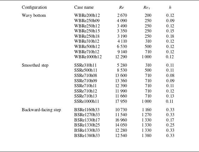
A summary of case name and parameters is provided in table 3. Additional details regarding numerical set-up can be found in Appendix B. For comparison purposes, we also simulate flow in the same configuration for the predicted cases using the standard RANS model with the
 $k$
–
 $\epsilon$
and
 $k$
–
 $\omega$
closure models. These simulations were performed using the flow solver available in ANSYS Fluent, with all turbulence-related parameters set to their default values.
Summary of case names, values of the Reynolds number (
 $ \textit{Re}$
), frictional Reynolds number (
 $ \textit{Re}_\tau$
) and geometric feature (h) for all the LES simulations cases. Case names use the prefixes ‘WB’, ‘SS’ and ‘BS’ for the four-periodic wavy bottom, smoothed step and backward-facing step cases, respectively.

The stream function
 $\psi$
is obtained by solving the Laplace equation,
 ${\nabla} ^2 \psi = 0$
, subject to the following boundary conditions:
 $\psi = 0$
along the bottom wall and
 $\psi = 1$
along the top boundary, with no horizontal variation at both the inlet and outlet boundaries. The velocity potential
 $\phi$
is similarly determined by solving the Laplace equation,
 ${\nabla} ^2 \phi = 0$
, with zero normal gradient imposed on the top and bottom boundaries. In addition, a Dirichlet condition
 $\phi = 0$
is applied at the left boundary, while at the right boundary,
 $\phi$
is set equal to the non-dimensional domain length (i.e.
 ${\rm d}\phi /{\rm d}x = 1$
).
The a posteriori simulations are conducted using FEniCSx, an open-source finite-element method framework for solving partial differential equations (Logg, Mardal & Wells Reference Logg, Mardal and Wells2012). FEniCSx is selected as the a posteriori flow solver primarily due to its flexibility, which facilitates the modification of turbulence closure models and the integration of our TBNN framework. Nevertheless, we believe that the current TBNN model can be incorporated into other open-source CFD solvers in a straightforward manner.
To obtain the solution of the RANS equations, the Newton–Raphson method is employed. In the following simulations, we use approximately 27 000, 60 000 and 81 000 elements for the wavy bottom, smoothed step and backward-facing step cases, respectively. The mesh is refined near both the top and bottom boundaries, with the finest and coarsest mesh sizes being approximately
 $0.01H$
and
 $0.04H$
, respectively, across all configurations.
5. Results and discussion
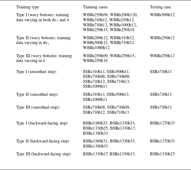
This section presents both a priori and a posteriori evaluations across three representative geometrical configurations. As summarised in table 3, the training dataset includes variations in both the friction Reynolds number (
 $ \textit{Re}_{\tau }$
) and the geometric parameter
 $h$
. Based on these variations, we consider three types of training data. The first type includes combined variations in both
 $ \textit{Re}_{\tau }$
and
 $h$
(type I), the second type includes variations in
 $ \textit{Re}_{\tau }$
only (type II), and the third includes variations in
 $h$
only (type III). Details of these variations are provided in table 4.
Summary of training and testing datasets corresponding to configuration cases and training types. Detailed information for each case is provided in table 3.

Each configuration is evaluated using two TBNN variants. The first variant, TBNN-i5, uses five local invariant-based features, following the original TBNN framework (Ling et al. Reference Ling, Jones and Templeton2016a
,Reference Ling, Kurzawski and Templeton
b
). The second variant, TBNN-i7, incorporates both the velocity potential and stream function values. Detailed comparisons through a priori and a posteriori evaluations are presented for the first type of training data, which include combined variations in
 $ \textit{Re}_{\tau }$
and
 $h$
. To keep the presentation concise, only a posteriori comparisons are provided for the second and third training cases. These comparisons involve the TBNN-i7 model, conventional RANS turbulence models and LES data. As previously mentioned, for the evaluation of a posteriori in each case, we compared the results with those obtained using traditional turbulence closure models,
 $k{-}\epsilon$
and
 $k\!-\!\omega$
. However, for the sake of conciseness, we present only the model that best matches our LES mean flow results for the flow field comparison.
5.1. Channel flow with a four-period wavy bottom
Figure 2 presents the mean flow patterns predicted by the four different model approaches, represented by the mean velocity magnitudes and streamlines, at the trough of the wavy bed. Figure 2(a) shows that the flow separates at the lee side of the wave, forming a recirculation zone, and reattaches at the windward side of the following wave crest. This type of bottom geometry has been frequently used to mimic periodically varying bed geometries in various geophysical flow problems. Accurately capturing the separation zone using traditional closure models is challenging but essential for predicting the associated form drag. This geometry was also used as a demonstration case in the pioneering TBNN study by Ling et al. (Reference Ling, Kurzawski and Templeton2016b ). In what follows, we first focus on predicting the anisotropic Reynolds stress tensor and eddy viscosity in the a priori stage, and return to the predicted mean velocity field in the a posteriori stage.
5.1.1. A priori evaluation with training data varying in both
$ \textit{Re}_{\tau }$
and
$h$


Figure 3 compares the predicted
 $b_{12}$
from the present TBNN model with those obtained from the LES mean flow field for the wavy-bottom case. Both TBNN-i7 and TBNN-i5 are able to predict the anisotropic tensor in the free stream region (i.e.
 $y \gt 0.3$
). However, only TBNN-i7 successfully captures its negative distribution observed in LES results (figure 3
b), which corresponds to the shear layer region above the recirculation zone. In contrast, TBNN-i5 predicts a significantly smaller and fragmented negative region (figure 3
c), indicating that it fails to reproduce the directional structure of the Reynolds stress in this zone. Although not shown here, similar trends are observed for the other anisotropic stress components,
 $b_{11}$
and
 $b_{22}$
.
Streamlines overlaid on velocity magnitude contours in the near-wall region for wave-bottom channel flow, shown for (a) LES data, and RANS results using (b) the
 $k$
–
 $\epsilon$
model, (c) the TBNN-i7 model and (d) the TBNN-i5 model.

Distributions of the anisotropic Reynolds stress tensor
 $b_{12}$
for the wavy-bottom case from (a) the original LES data, (b) TBNN-i7 prediction and (c) TBNN-i5 prediction.

Comparison of eddy viscosity distributions in the case with wavy-bottom channel flow obtained from (a) LES, (b,c) TBNN-i7 and (d,e) TBNN-i5. Panels (c) and (e) show the eddy viscosity fields obtained from the regression model (i.e. Random Forest).

The comparison of eddy viscosity fields further highlights the differences in predictive capabilities among models. Figure 4 presents the predicted eddy viscosities,
 $\nu _{t, {opt}}^\dagger$
and
 $\nu _{t,\textit{reg}}^\dagger$
. Here,
 $\nu _{t,\textit{reg}}^\dagger$
is obtained through regression using the Random Forest model, (2.19). In LES,
 $\nu _{t, {opt}}^\dagger$
is computed using (2.18) directly from the LES mean flow field of the predictive case, while in TBNN,
 $\nu _{t, {opt}}^\dagger$
is also calculated using (2.18) but based on data predicted from training cases in table 4. From the LES results, as shown in figure 4(a), it is observed that the eddy viscosity significantly decreases within the recirculation zone downstream of each crest, while a sharp increase appears in the free shear layer above, forming a high eddy viscosity region.
The optimised eddy viscosity fields reconstructed from the TBNN-predicted Reynolds stress tensors show that TBNN-i7 (figure 4
b) successfully reproduces the characteristic LES structure. It is worthwhile to mention that although our sampling size ensures the statistical convergence of the mean flow field in LES, the second-moment quantities, such as
 $b_{12}$
in figure 3(a), still exhibit slight irregularities. Such irregularities are even more apparent in
 $\nu _t$
, as shown in figure 4(a), as it is obtained by dividing the mean velocity gradient. The same features can also be found in the other two examples. While such issues could be improved by extending the sampling size (i.e. a longer period of sampling time), as shown in figure 4(b), these small-scale irregularities can be effectively filtered out by the present TBNN.
In contrast to TBNN-i7, as shown in figure 4(d), TBNN-i5 introduces spurious extrema within the recirculation zone. These results demonstrate that the inclusion of geometric features in TBNN-i7 enhances its ability to capture eddy viscosity variations in inhomogeneous regions, compared with the limited expressiveness of TBNN-i5. In addition, as shown in figures 4(c) and 4(e), the eddy viscosity fields predicted by the regression model show strong consistency with the TBNN results (figures 4 b and 4 d, respectively), confirming the effectiveness of our regression model.
Convergence behaviour of the iterative solution process used to compute velocity profiles for the wavy-bottom channel flow, shown over a single geometric period. (a) Evolution of the velocity field across selected iterations. (b) Histograms of the residuals defined in (5.1) at the 1st, 3rd and 10th iteration steps, with colours corresponding to those in panel (a).

5.1.2. A posteriori evaluation with training data varying in both
$ \textit{Re}_\tau$
and
$h$


Since ensuring solution convergence during iteration is a key aspect of the flow solver, we examine convergence in figure 5. This figure presents the calculated velocity profiles at representative iteration steps towards the steady-state solution, along with the corresponding histograms of residuals. The residual at the
 $m$
th iteration step during the iterative process is defined as
 \begin{align} r_n^{(m)} =\dfrac {1}{\mathcal{U}}\big (\boldsymbol{U}_n^{(m)}-\boldsymbol{U}_{n, \textit{ref}}\big ), \end{align}
where
 $n$
is the index of the grid point and the subscript
 $ref$
denotes the reference value. In figure 5, we use the iterative solution at the
 $85$
th step as the reference. As shown in figure 5(a), the velocity profiles converge after just a few iteration steps. Moreover, figure 5(b) illustrates that the residuals evolve toward a normal distribution centred near zero as the iteration progresses. In this study, the iteration process is terminated when the following convergence criterion is satisfied:
 \begin{align} \dfrac {\big \Vert \boldsymbol{U}^{(m)}-\boldsymbol{U}^{(m-1)}\big \Vert _2}{\big \Vert \boldsymbol{U}^{(m-1)}\big \Vert _2} \lt 10^{-10}\,, \end{align}
where the superscript
 $(k)$
indicates the iteration step.
Figure 6 presents the predicted velocity profiles obtained from LES, TBNN,
 $k\!-\!\epsilon$
and
 $k-\omega$
closure models at various streamwise locations. As shown in figure 6, all models exhibit steep velocity gradients near the wall, indicating a consistent ability to capture viscosity-dominated regions. However, both TBNN-i5 and
 $k\!-\!\omega$
tend to overpredict the velocity profiles, whereas TBNN-i7 and
 $k{-}\epsilon$
more closely match the LES results. The discrepancies observed in the traditional closures (i.e.
 $k$
–
 $\epsilon$
and
 $k$
–
 $\omega$
) are mainly attributed to the misprediction of near-wall turbulent viscosity. While we adopt the default values in ANSYS Fluent for the empirical coefficients in the transport equations of the second-moment quantities (i.e.
 $k$
,
 $\epsilon$
and
 $\omega$
), these discrepancies could potentially be mitigated by tuning those empirical values. Such considerations, however, fall outside the scope of the present study. Here and in thefollowing numerical tests, we focus on discussing the TBNN-based methods and include the traditional closure models primarily for reference.
The overprediction in TBNN-i5 arises from its inability to yield a
 $b_{12}$
field with sufficient accuracy in the near-wall region. As shown in figure 3, compared with the original LES data and the prediction by TBNN-i7, TBNN-i5 (figure 3
c) fails to accurately capture the decrease in
 $b_{12}$
towards the wall boundary. This leads to an overall overprediction of the anisotropic Reynolds stress in the near-wall region. Although both TBNN-i7 and TBNN-i5 produce eddy viscosity values similar to the original LES results, as shown in figure 4, the overprediction of
 $b_{12}$
in the latter case results in an overestimation of the mean velocity profile, as illustrated in figure 6. In the near-wall region behind the crest, where flow separation occurs, TBNN-i7 outperforms the other three models (see the inset), but slightly underperforms
 $k$
–
 $\epsilon$
on the crest.
In addition, the flow patterns represented by the velocity magnitudes and streamlines within the separation and reattachment regions presented in figure 2 further highlight the differences among model predictions. As shown in figure 2(a), the LES results exhibit a typical shear layer and recirculation structure, accompanied by noticeable streamline deflection. This recirculation is a classical manifestation of flow separation driven by an adverse pressure gradient. In comparison, as shown in figure 2(b),
 $k$
–
 $\epsilon$
shows the main flow closely attached to the wall, with minimal recirculation behaviour. In figure 2(c), the flow field predicted by TBNN-i7 deviates slightly from the LES results in the location of the shear layer, but successfully captures parts of the reverse flow and the reattachment region. As shown in figure 2(d), TBNN-i5 produces qualitatively similar results to TBNN-i7, but overpredicts both the free stream velocity and the extent of the recirculation zone. These observations indicate that both TBNN models outperform the
 $k$
–
 $\epsilon$
closure model in capturing separated flow features, with the inclusion of spatial and geometric descriptors in TBNN-i7 significantly improving flow prediction accuracy.
Comparison of velocity profiles from different simulation approaches in the case of wavy-bottom channel flow.

In addition to the velocity field, we also compare the modelled friction coefficient among different simulation cases. The bottom drag coefficient is obtained by calculating the bottom drag using the non-dimensional quantities,
 \begin{align} C_{\kern-1.5pt f} = \left (\nu +\nu _t\right )\dfrac {{\rm d}\vert \boldsymbol{U} \vert }{{\rm d}\xi }\Bigg \vert _{btm}, \end{align}
where
 $\vert \boldsymbol{U} \vert = \sqrt {U_1^2+U_2^2}$
,
 $\xi$
represents the distance along the direction normal to the bottom geometry and the subscript
 $btm$
indicates the bottom boundary. In this study, a second-order finite difference scheme that incorporates the no-slip boundary condition and the first two grid points from the bottom is employed to approximate the values of
 $C_{\kern-1.5pt f}$
.
Figure 7 presents a comparison of
 $C_{\kern-1.5pt f}$
among the different simulation approaches. The results from the TBNN model exhibit non-physical fluctuations. This occurs because the pointwise eddy viscosity obtained from the TBNN can lead to non-smoothness in the predicted eddy viscosity field, which in turn induces fluctuations in the resulting velocity field. These fluctuations become particularly evident when examining the near-bed shear stress. Applying an appropriate smoothing procedure to the TBNN-generated eddy viscosity, while preserving the global extrema, could help mitigate this issue in future work. Compared with the LES result, the TBNN-i7 case shows slight overprediction of drag at the lee side, but underprediction at the trough and windward side, whereas the TBNN-i5 case shows overprediction near the peak. Flow reattachment can be assessed by the
 $x$
-location where
 $C_{\kern-1.5pt f} = 0$
, indicated by the dashed lines. The
 $k$
–
 $\epsilon$
model fails to capture drag reversal at the lee and windward sides due to its inability to predict flow separation, consistent with figure 2(b). Compared with LES, predicted reattachment occurs slightly upstream in TBNN-i7 and slightly downstream in TBNN-i5. Despite these discrepancies, in contrast to the
 $k$
–
 $\epsilon$
model, both TBNN-i5 and TBNN-i7 capture the overall pattern of drag reflection associated with flow detachment and reattachment, although the locations of reflection are slightly shifted relative to the LES result.
Comparison of the bottom friction coefficient (
 $C_{\kern-1.5pt f}$
) from different simulation approaches in the case of wavy-bottom channel flow. The dash lines indicate the locations where the separated flow reattaches in each case.

5.1.3. A posteriori evaluation with training data varying in either
$ \textit{Re}_\tau$
or
$h$


Figure 8 shows the comparison of predicted mean velocity profiles from LES data and various models for cases trained with data that vary either
 $ \textit{Re}_{\tau }$
or
 $h$
in the wavy-bottom configuration. Overall, both TBNN-i7 and
 $k$
–
 $\omega$
show good agreement with the LES results for both training types. However, in the near-wall region on the lee side of the bottom wave (
 $x \sim 0.3$
), the TBNN-i7 model produces velocity profiles that are closer to the LES data compared with those from the
 $k$
–
 $\omega$
model. The good performance of TBNN-i7 is consistent with the results observed in the combined variation training cases, as shown in figure 6, which further confirms the capability of the TBNN-i7 model in handling variations in both free stream flow and geometry.
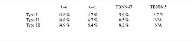
Summary of global error values (
 $E$
), as defined in (5.4), for the
 $k$
–
 $\epsilon$
,
 $k$
–
 $\omega$
and TBNN-i7 models in the four-period wavy-bottom channel flow case, using different training data types.

Comparison of velocity profiles from different simulation approaches in the case of wavy-bottom channel flow with training data across either various (a)
 $ \textit{Re}_{\tau }$
(type II) or (b)
 $h$
(type III).

A more quantitative assessment for different models is made by comparison of global errors among different models. The global error (
 $E$
) is defined as
 \begin{align} E=\dfrac {\displaystyle {\sum ^N_{n=1}}\big \vert \boldsymbol{U}_{\!\textit{LES},n}-\boldsymbol{U}_n\big \vert \Delta _n}{\displaystyle {\sum ^N_{n=1}}\big |\boldsymbol{U}_{\!\textit{LES},n}\big |\Delta _n}\,, \end{align}
where
 $\boldsymbol{U}_{\!\textit{LES}}$
denotes the velocity field obtained from LES,
 $n$
is the grid index,
 $\Delta$
is the area of the grid cell and the summation is taken over the
 $N$
grid points used for training the TBNN model. Table 5 summarises the global errors (
 $E$
) for the results obtained using the TBNN-i7 and traditional turbulence closure methods for the wavy-bottom case. It can be seen that
 $E \lt 10\,\%$
for both the TBNN-i7 and
 $k$
–
 $\epsilon$
models when evaluated on training data that varies in both
 $ \textit{Re}_\tau$
and
 $h$
(type I). When the training data varies in only one of the two parameters, either
 $ \textit{Re}_\tau$
or
 $h$
(types II and III, respectively), the present TBNN-i7 model still achieves good agreement with the LES results (
 $E \lt 10\,\%$
). In contrast, neither the
 $k$
–
 $\epsilon$
nor the
 $k$
–
 $\omega$
model is able to provide accurate predictions, primarily due to significant discrepancies in the near-wall region on the lee side.
5.2. Flow over a smoothed step
Figure 9 presents the mean flow patterns predicted by the four model approaches, represented by the mean velocity magnitude and streamlines, in a representative case of flow over a smoothed step. Figure 9(a) shows that the flow separates at the downslope ramp (
 $x \sim 6.0$
) and reattaches further downstream, forming a recirculation zone. The smoothed ramp configuration serves as a canonical case for studying turbulent separation induced by an adverse pressure gradient in the absence of sharp geometric discontinuities. This makes it highly representative of many real-world engineering flows such as aerofoils, diffusers and internal ducts, where separation is driven primarily by a smooth geometry-induced adverse pressure gradient, rather than sudden expansions. Accurately predicting flow behaviour in such conditions remains a significant challenge for turbulence models, particularly in capturing the onset of separation and reattachment under varying pressure gradients (e.g. Simmons et al. Reference Simmons, Thomas, Corke and Gluzman2024).
Streamlines overlaid on velocity magnitude contours in the near-wall region for the case of flow over a smoothed step, shown for (a) LES data, and RANS results using (b) the
 $k$
–
 $\omega$
model, (c) the TBNN-i7 model and (d) the TBNN-i5 model.

5.2.1. A priori evaluation with training data varying in both
$ \textit{Re}_\tau$
and
$h$


In the smoothed-step case, the predicted anisotropic Reynolds stress tensor behaves similarly to that observed in the four-period wavy-bottom case, with TBNN-i7 exhibiting higher accuracy than TBNN-i5. As such, the following discussion focuses on comparisons of eddy viscosity. Figure 10 presents the predicted eddy viscosities,
 $\nu _{t, {opt}}^\dagger$
and
 $\nu _{t, {reg}}^\dagger$
, using the present TBNN model alongside those obtained from the LES mean flow field. The LES results in figure 10(a) indicate a low eddy viscosity region near the leading edge of the smoothed step, reflecting a typical acceleration zone. A high eddy viscosity zone appears downstream of the step, corresponding to the free shear layer generated by flow separation. This region is characterised by strong turbulent mixing and momentum exchange. Near the bottom wall, the eddy viscosity decreases to nearly zero. Figure 10(b) shows that TBNN-i7 successfully reconstructs these key features, yielding a distribution that closely matches the LES and eliminates small-scale fluctuations present in the original LES data. In contrast, TBNN-i5, as shown in figure 10(d), captures the general trend in the free stream region, but underpredicts the eddy viscosity in most of the places except for the upper free stream region behind the step. As shown in figures 10(c) and 10(e), the eddy viscosity fields obtained from the Random Forest regression model are also highly consistent with the original TBNN-i7 and TBNN-i5 outputs.
Comparison of eddy viscosity distributions obtained by different methods in the case of flow over a smoothed step: (a) original LES result; (b) and (d) predictions by TBNN-i7 and TBNN-i5, respectively; (c) and (e) eddy viscosity fields obtained by the Random Forest regression model in cases of TBNN-i7 and TBNN-i5, respectively.

Comparison of velocity profiles from different simulation approaches in the case of flow passing a smoothed step.

5.2.2. A posteriori evaluation with training data varying in both
$ \textit{Re}_\tau$
and
$h$


Figure 11 presents the streamwise velocity profiles predicted by different models. It can be seen that the
 $k$
–
 $\epsilon$
model significantly underpredicts the velocity magnitude, likely due to its overprediction of the eddy viscosity. This results in the absence of backflow at the downslope ramp, as shown in the inset of figure 11. Another misprediction at the downslope ramp is also observed in the TBNN-i5 profile, which exhibits an unphysical velocity drop towards the bottom (see the inset). This behaviour is consistent with the mispredicted recirculation pattern shown in figure 9(d). Overall, the TBNN-i7 prediction shows good agreement with the LES results, accurately capturing the velocity curvature from upstream to the top of the step and maintaining a reasonable near-wall velocity gradient. However, the
 $k$
–
 $\omega$
model outperforms TBNN-i7 at the downslope ramp, yielding a velocity profile that more closely matches the LES result in that region, though it overestimates the velocity in the free stream core region.
Further examination of the separated and reattached flow structures shown in figure 9 reveals notable differences between different approaches. The LES result in figure 9(a) shows a stable recirculation bubble, corresponding to the shear layer and a reverse flow structure driven by the adverse pressure gradient. The
 $k\!-\!\omega$
closure method shown in figure 9(b) clearly captures the internal details of the recirculation closely matching the LES data. TBNN-i7, as shown in figure 9(c), reproduces the overall shape of the shear layer and recirculation bubble, although the size of the recirculation is smaller and the velocity gradient appears smoother than in LES. TBNN-i5, as shown in figure 9(d), shows a similar trend to TBNN-i7, but with an irregular recirculation pattern. Overall, while the TBNN-based models exhibit limitations in capturing fine-scale turbulent mixing, they successfully reconstruct the main flow features. For an overall assessment, as shown in table 6 (type I), both TBNN-i7 and
 $k\!-\!\omega$
can achieve
 $E \lt 10\,\%$
.
Summary of global error values (
 $E$
), as defined in (5.4), for the
 $k$
–
 $\epsilon$
,
 $k$
–
 $\omega$
and TBNN-i7 models in the case of flow over a smoothed step, using different training data types.

Figure 12 presents a comparison of the bottom friction coefficient (
 $C_{\kern-1.5pt f}$
) among different modelling approaches for the smoothed-step case. Upstream of the downslope ramp, all approaches capture the overall spatial distribution of
 $C_{\kern-1.5pt f}$
, with a slight underprediction on the upslope ramp and an overprediction on the step. As in the previous wavy-bottom example, the TBNN results exhibit noticeable fluctuations. More substantial differences among the modelling approaches appear in the downstream region adjacent to the downslope ramp, as highlighted in the inset of the figure. The increase in bottom friction associated with the circulation zone, clearly observed in the LES results, is well reproduced by the
 $k$
–
 $\omega$
model, but underpredicted by TBNN-i7 due to its underestimated circulation region (see figure 9
c). Consequently, TBNN-i7 predicts an upstream-shifted reattachment point, whereas
 $k$
–
 $\omega$
aligns more closely with the LES result, as indicated by the dashed lines. TBNN-i5 fails to capture this friction increase because it does not correctly reproduce the circulation zone (see figure 9
d).
Comparison of the bottom drag coefficient (
 $C_{\kern-1.5pt f}$
) from different simulation approaches in the case of smoothed-step channel flow. The dash lines in the inset indicate the locations where the separated flow reattaches in each case.

5.2.3. A posteriori evaluation with training data varying in either
$ \textit{Re}_{\tau }$
or
$h$


Figure 13 shows the comparison of predicted mean velocity profiles from LES data and various models with training data varying in either
 $ \textit{Re}_{\tau }$
or
 $h$
in the smoothed-step configuration. Here, we focus on the downstream half of the domain, containing the downslope ramp. In the case with varying
 $ \textit{Re}_{\tau }$
, as shown in figure 13(a), TBNN slightly underpredicts the external flow region while the
 $k$
–
 $\omega$
model slightly overpredicts it. In the near-wall region right behind the downslope ramp (
 $x \approx 6$
), the TBNN-i7 tends to slightly underpredict the reverse flow, whereas the
 $k$
–
 $\omega$
model results agree more closely with the LES data. However, at the further downstream location (
 $x \approx 7$
), the TBNN-i7 results align well with the LES data near the wall, while the
 $k$
–
 $\omega$
model shows more discrepancies. Despite these slight deviations, both TBNN-i7 and
 $k$
–
 $\omega$
show good agreement with the LES data when variations in
 $ \textit{Re}_{\tau }$
are used for training. This is also reflected in table 6, which shows that the global errors in both cases are less than
 $10\,\%$
.
When variations in the geometric feature
 $h$
are used for training, as shown in figure 13(b), the TBNN-i7 again produces results that closely match the LES data, except for a slight underprediction of reverse flow behind the step (
 $x \approx 6$
), similar to the previous case (figure 13
a). As indicated in table 6, the error in TBNN-i7 reaches
 $2.9\,\%$
.
Comparison of velocity profiles from different simulation approaches in the case of flow over a smoothed step with training data across either various (a)
 $ \textit{Re}_{\tau }$
(type II) or (b)
 $h$
(type III).

5.3. Backward-facing step
The third case considers the flow field induced by a backward-facing step. Figure 14 presents the mean flow patterns predicted by four different model approaches, represented by the mean velocity magnitude and streamlines, in a representative case of this configuration. Figure 14(a) shows that this geometric configuration causes strong flow separation immediately at the corner of the step, forming a large-scale recirculation zone and a distinct shear layer. Compared with the previous two cases, this configuration features the farthest downstream reattachment point and represents the challenging scenario for prediction. Flows over a backward-facing step have been widely studied in the literature (e.g. Geneva & Zabaras Reference Geneva and Zabaras2019; Beetham & Capecelatro Reference Beetham and Capecelatro2020; Agrawal & Koutsourelakis Reference Agrawal and Koutsourelakis2024).
Streamlines overlaid on velocity magnitude contours in the near-wall region for the case of flow over a backward-facing step, shown for (a) LES data, and RANS results using (b) the
 $k$
–
 $\omega$
model, (c) the TBNN-i7 model and (d) the TBNN-i5 model.

5.3.1. A priori evaluation with training data varying in both
$ \textit{Re}_\tau$
and
$h$


In the backward-facing step case, TBNN-i7 continues to show good agreement with LES in predicting the anisotropic Reynolds stress tensor, while TBNN-i5 presents noticeable deviations. As these results are consistent with previous cases, the following analysis focuses on the eddy viscosity distribution. Figure 15 presents the eddy viscosities obtained from different model strategies analogous to figure 10. Compared with the LES results (figure 15 a), TBNN-i7 (figure 15 b) successfully reproduces the distribution of the eddy viscosity, accurately capturing the low eddy viscosity characteristics behind the step and the local maxima near the reattachment region. In contrast, although TBNN-i5 (figure 15 c) captures the overall trend around the step, it underpredics the increase in eddy viscosity outside the boundary layer. As shown in figures 15(d) and 15(e), the eddy viscosity fields obtained by the regression model remain highly consistent with the original TBNN-i7 and TBNN-i5 outputs.
Comparison of eddy viscosity distributions obtained by different methods in the backward-facing step channel flow: (a) original LES result; (b) and (d) predictions by TBNN-i7 and TBNN-i5, respectively; (c) and (e) eddy viscosity fields obtained by the regression model in cases of TBNN-i7 and TBNN-i5, respectively.

5.3.2. A posteriori evaluation with training data varying in both
$ \textit{Re}_{\tau }$
and
$h$


Figure 16 presents the streamwise velocity profiles predicted by different models. It shows that both TBNN-i7 and
 $k$
–
 $\omega$
exhibit robust predictive performance, closely matching the LES results in most places except that the former slightly underpredicts the flow reversal at the downstream separation behind the step (see the inset) and the latter slightly underpredicts the flow at the downstream reattachment point (
 $x \approx 12$
). Due to the misprediction of the eddy viscosity in the vicinity of the wall, neither TBNN-i5 nor
 $k$
–
 $\epsilon$
accurately predicts the boundary-layer thickness, leading to an underprediction of the velocity above the boundary layer. As summarised in table 7, both TBNN-i7 and
 $k\!-\!\omega$
achieve the global error
 $E \lt 10\,\%$
with the latter being slighly lower, while
 $k$
–
 $\epsilon$
remains
 $E \sim O(10\,\%)$
.
Summary of global error values (
 $E$
), as defined in (5.4), for the
 $k$
–
 $\epsilon$
,
 $k$
–
 $\omega$
and TBNN-i7 models in the backward-facing step case, using different training data types.

As highlight by streamlines overlying the velocity magnitudes, figure 14 allows the further inspection of the separation and reattachment structures. As shown in figure 14(a), the LES result exhibits a well-defined recirculation bubble and shear layer behind the step, representing a typical separation driven by an adverse pressure gradient. The
 $k\!-\!\omega$
prediction shown in figure 14(b) agrees well with LES in the near-wall velocity distribution, but exhibits slight discrepancies in the location and extent of the recirculation bubble. TBNN-i7 shown in figure 14(c) successfully reconstructs both the recirculation and reattachment structures, with a velocity field that closely resembles LES. TBNN-i5 shown in figure 14(d) also identifies the main separated and recirculation regions, but the depth of the recirculation bubble and the reattachment location are slightly shifted further downstream. Overall, TBNN-i7 provides accurate near-wall velocity predictions, while TBNN-i5 and
 $k$
–
 $\omega$
maintain consistent reconstruction of the overall structure, but remain less accurate in predicting the reattachment location.
Comparison of velocity profiles from different simulation approaches in the case of flow passing a backward-facing step.

Figure 17 presents a comparison of the bottom friction coefficient (
 $C_{\kern-1.5pt f}$
) among different modelling approaches for the backward-facing step flow. On the step’s upper flat surface, the predicted drag coefficients generally agree well with the LES results, except that TBNN-i7 slightly underpredicts
 $C_{\kern-1.5pt f}$
, and all TBNN-based methods exhibit fluctuations, consistent with the previous two examples. Downstream of the backward-facing step,
 $C_{\kern-1.5pt f}$
drops to zero and then gradually increases to a peak due to flow circulation inside the separation bubble. The friction coefficient subsequently decreases to zero at flow reattachment. In general, TBNN-i5 overpredicts
 $C_{\kern-1.5pt f}$
downstream of the step, primarily due to overestimation of the eddy viscosity near the wall in this region, as shown in figure 15(e). Both
 $k\!-\!\omega$
and TBNN-i7 capture the magnitude of the drag increase induced by circulation. As indicated by the dashed lines, the reattachment points predicted by the TBNN-based methods are shifted slightly downstream relative to the LES result. In the
 $k$
–
 $\omega$
case, the reattachment point is located even farther downstream (
 $x \approx 12$
), consistent with the delayed reattachment observed in figure 14(b). Downstream of reattachment, both
 $k$
–
 $\omega$
and TBNN-i7 underpredict the friction coefficient, while TBNN-i5 shows overprediction.
Comparison of the bottom drag coefficient (
 $C_{\kern-1.5pt f}$
) from different simulation approaches in the case of backward-facing step flow. The dash lines indicate the locations where the separated flow reattaches in each case.

5.3.3. A posteriori evaluation with training data varying in either
$ \textit{Re}_{\tau }$
or
$h$


Figure 18 presents a comparison of the predicted mean velocity profiles from LES data and various models, using training data that vary either in
 $ \textit{Re}_{\tau }$
or in
 $h$
, for the backward-facing step configuration. As shown in figure 18(a), TBNN-i7 underpredicts the free shear layer immediately downstream of the step at
 $x \approx 9.5$
, while the
 $k$
–
 $\omega$
model slightly overpredicts the velocity shear further downstream at
 $x \approx 10$
. Despite these minor deviations from the LES data, both TBNN-i7 and the
 $k$
–
 $\omega$
model show good agreement with the LES results. As indicated in table 7, the global errors for both models are less than
 $10\,\%$
, whereas the
 $k$
–
 $\epsilon$
model exhibits significantly larger error. When training data vary in
 $h$
, the discrepancy between TBNN-i7 predictions and LES results becomes more pronounced immediately behind the step, leading to a slightly higher global error compared with the type II training case, as shown in table 3. Nevertheless, both TBNN-i7 and the
 $k$
–
 $\omega$
model effectively capture the overall trend of the velocity field in the backward-facing step configuration.
Summary of global error values (
 $E$
), as defined in (5.4), for the cases using combined type I training data across different geometries, along with the values from TBNN-i7 for comparison.

Comparison of velocity profiles from different simulation approaches in the case of backward-facing step with training data across either various (a)
 $ \textit{Re}_{\tau }$
(type II) or (b)
 $h$
(type III).

5.4. Combination of different bottom geometries
Having demonstrated the applicability of the present TBNN framework to flows over three types of bottom geometry, we now assess its potential and limitations across different geometries. For this, all type I training data from the various geometries are used to predict the type I testing cases for each individual geometry, as summarised in table 4.
We consider three training strategies. The first uses the proposed seven flow features (
 $\lambda _{1-5}$
,
 $\phi$
and
 $\psi$
) across all geometries, denoted TBNN-C-i7. The second adopts the original TBNN with five features (
 $\lambda _{1-5}$
) without
 $\phi$
and
 $\psi$
, denoted TBNN-C-i5, to evaluate the effect of the additional input features on model generalisation. The third strategy uses the seven features, but adds one-hot encoding for geometry:
 $[1\ 0\ 0]$
for the wavy bottom,
 $[0\ 1\ 0]$
for the smoothed step and
 $[0\ 0\ 1]$
for the backward-facing step, referred to as TBNN-C-i7oh. We focus on strategies that can be readily extended from the current framework. While advanced encoding techniques exist, this study provides a preliminary assessment of geometric generalisation without exploring alternative encoding approaches.
Figure 19 presents a comparison of the predicted velocity profiles for three different bottom geometries using the aforementioned training strategies, together with the results from TBNN-i7 and LES. For a more quantitative assessment, table 8 summarises the prediction errors (
 $E$
) within the near-wall regions shown in figures 2, 9 and 14, along with those from TBNN-i7 for reference. From figure 19 and table 8, it can be seen that TBNN-C-i7 performs poorly, showing large deviations from the LES results in all three geometric cases. In contrast, and different from the results obtained when training with individual geometries, the prediction from TBNN-C-i5 is significantly improved when the stream function and velocity potential are excluded. In this case, the global error is reduced to less than 10
 $\,\%$
in the wave-bottom and smoothed-step cases, although it remains large for the backward-facing step (figure 19
c).
Predicted velocity profiles for the three bottom geometries using the combined-dataset training strategies TBNN-C-i5, TBNN-C-i7 and TBNN-C-i7oh, shown together with the predictions from TBNN-i7 and the LES results.

The deterioration in prediction when including
 $\psi$
and
 $\phi$
arises because these two additional features tend to limit the model applicability to the specific geometry used for training. Since their local values are not readily comparable across different geometries, combining datasets that include
 $\psi$
and
 $\phi$
can degrade TBNN prediction accuracy in varying geometries. Furthermore, because each geometry type in this study uses a distinct domain configuration, the absence of a unified domain definition may further worsen the predictions when these two features are included. This limitation may be mitigated by introducing additional features that better characterise the global geometry or by incorporating explicit geometric categorisation during training, as in the TBNN-C-i7oh model, which uses one-hot encoding to distinguish different geometry types. As shown in figure 19 and table 8, TBNN-C-i7oh yields noticeably improved velocity predictions. These results suggest that more advanced ML-based geometric encoding strategies may provide a promising direction for further enhancing the generalisability of the present TBNN framework.
6. Conclusion
In this study, we present an ML-based turbulence closure model that can be directly embedded into a RANS solver without relying on any baseline model calculations. The closure model is developed based on the theoretical framework of the algebraic eddy viscosity model proposed by Pope (Reference Pope1975) and the modern ML framework introduced by Ling & Templeton (Reference Ling and Templeton2015).
We propose two key contributions to address challenges encountered in both the a priori learning and a posteriori deployment stages of data-driven turbulence modelling. First, to enhance the expressiveness and robustness of the a priori model, we introduce geometry-informed features as additional inputs to the neural network. Specifically, in addition to the original local invariant features, we incorporate the stream function and velocity potential, both of which can be obtained straightforwardly before solving the governing equations. Combined with a rescaled eddy viscosity formulation, these additions eliminate the need for any baseline RANS model to obtain second-moment quantities.
For the a posteriori stage, we introduce a regression model using Random Forest to predict an appropriate eddy viscosity from given mean strain rates and anisotropic Reynolds stress tensors. This regression model is directly embedded into a RANS solver, allowing the flow solution to be computed iteratively in a manner similar to conventional turbulence models, without relying on any baseline model calculations. We present three canonical flow configurations, namely the wavy bottom, smoothed step and backward-facing step, to demonstrate the capabilities of our model in channel flow with a variety of bottom geometries. We demonstrate that incorporating stream functions and velocity potentials significantly improves the model’s predictive performance for the anisotropic stress tensor in the a priori stage. Furthermore, we show that the addition of the Random Forest regression model effectively predicts eddy viscosities.
While in the a posteriori evaluation, our TBNN model consistently delivers accurate predictions of the mean flow field when compared with the LES datasets, several open issues require further development and improvement. First, because RANS does not account for the anisotropic nature of turbulence, incorporating anisotropy, either by adopting an anisotropic eddy viscosity or by introducing an external source term, could be a potential improvement. However, how these additions affect solution convergence in the a posteriori stage warrants further investigation. Second, although we focus on channel flows in this study, extending the model to a broader variety of flow configurations remains an important direction for future research. In particular, the use of the stream function and velocity potential in external flows (e.g. flow around blunt bodies) or in three-dimensional flows may differ from the present setting. Third, while we have demonstrated simple training and prediction across different geometries, incorporating advanced ML techniques for categorising or mapping complex geometries could be a crucial component for future development.
Despite the need for further exploration to broaden the applicability of the present model, this study presents the first ML-based turbulence closure framework that eliminates the need for baseline model calculations. The proposed two-layer ML architecture, which combines TBNN with a regression model, offers a novel structure for ML-based turbulence closure.
Acknowledgements
The authors gratefully acknowledge the National Center for High-performance Computing (NCHC), National Applied Research Laboratories (NARLabs), Taiwan, for providing computational and storage resources.
Funding
This work was supported by the National Science and Technology Council (NSTC), Taiwan, under the Thermal Science and Fluid Dynamics Program (Grant Nos. 109-2221-E-002-028-MY3 and 112-2221-E-002-139-MY3) and the Ocean Engineering Division (Grant No. 112-2221-E-002-186-MY3).
Declaration of interests
The authors report no conflict of interest.
Appendix A. Neural network implementation
This study employs two learning components: a TBNN and an auxiliary regression model. The TBNN is responsible for predicting the dimensionless anisotropic Reynolds stress tensor, while the regression model provides a stable and consistent eddy viscosity estimate to enhance the robustness of the coupled RANS solver. This section outlines the preprocessing steps, network architectures and optimisation strategies for both components.
A crucial aspect of integrating machine learning (ML) into computational fluid dynamics (CFD) lies in the preprocessing of input data. To improve predictive accuracy, all input features are constrained to lie within a bounded range. For flow-related tensor quantities, it is essential to distinguish between non-dimensionalisation and feature scaling (Fang et al. Reference Fang, Zhao, Waschkowski, Ooi and Sandberg2023). In this study, all input features are first non-dimensionalised to ensure generalisability across different flow regimes and then scaled to the range
 $[0, 1]$
to mitigate numerical instabilities caused by large variations in magnitude. Since the tensor invariants and integrity basis tensors are constructed from the dimensionless strain-rate and rotation-rate tensors, whose magnitudes typically range from
 $O(1)$
to
 $O(10)$
, large disparities among features may dominate the network’s internal representation. To prevent any single feature from overwhelming the learning process, we normalise each component of the strain-rate and rotation-rate tensors by the maximum absolute value observed in the training dataset, ensuring their magnitudes do not exceed
 $O(1)$
. The normalised tensors are defined as
 $S_{\textit{ij}}^\ast / |S_{\textit{ij}}^\ast |_{\textit{max}}$
and
 $R_{\textit{ij}}^\ast / |R_{\textit{ij}}^\ast |_{\textit{max}}$
, where
 $|{\boldsymbol{\cdot}}|_{\textit{max}}$
denotes the maximum absolute value computed over the training samples.
To train the model, the flow field is sampled at discrete spatial locations to extract input–output vector pairs. These sampling points are generated from a finite-element mesh constructed using polygonal triangulation, with local refinement applied near boundaries to balance the distribution of feature magnitudes. For each flow field, approximately
 $4 \times 10^3$
to
 $5 \times 10^3$
training samples
 $N_t$
are collected. This procedure transforms the continuous flow field into a representative dataset suitable for supervised learning, containing input tensor features and the corresponding anisotropic tensors.
The proposed TBNN adopts a one-point training approach, in which each spatial location is treated independently using a multilayer, fully connected feed-forward network. The architecture consists of an input layer, several hidden layers and an output layer. The input layer maps the features to a hidden representation of prescribed width. Each hidden layer applies a linear transformation followed by a LeakyReLU activation function with a negative slope of 0.01, and the output layer yields the coefficients associated with the tensor basis. The overall structure is summarised as
 \begin{align} \texttt {Input} \to [\texttt {Linear} \to \texttt {LeakyReLU}]^{(L-2)} \to \texttt {Linear (Output)}\,, \end{align}
where
 $L$
is the total number of layers, which is treated as a tuneable hyperparameter along with the hidden-layer width.
The model is implemented in PyTorch. To identify an optimal set of hyperparameters, the Optuna framework is employed to perform 50 optimisation trials. The tuneable parameters include the hidden-layer width (ranging from 60 to 180), the number of layers (between 5 and 10), the number of training epochs (200 to 800), batch size (16 to 256), learning rate (from
 $10^{-4}$
to
 $10^{-2}$
in logarithmic scale) and optimiser type (either Adam or SGD). The optimiser is dynamically selected using Optuna’s categorical suggestion mechanism and instantiated via Python’s getattr interface. To prevent overfitting and reduce computational cost, an early stopping criterion is applied: training is terminated if no improvement is observed in the validation loss for 50 consecutive epochs. This optimisation strategy allows efficient exploration of the hyperparameter space while maintaining model generalisation. Once the optimal hyperparameters are identified, the training data are partitioned into 20 subsets for
 $K$
-fold cross-validation. This strategy is employed to improve the generalisation capability of the trained TBNN model. During the training phase, each fold is used as a validation set, while the remaining folds serve as the training data, ensuring that every sample contributes to both training and validation. In the inference stage, the final prediction is obtained by averaging the outputs of the 20 independently trained models. This ensemble approach helps to reduce variance and enhance the robustness of the TBNN predictions.
Comparison of the simulated mean velocity profiles at representative streamwise locations between case WBRe500h12 in the present LES dataset and the results of Calhoun & Street (Reference Calhoun and Street2001).

Additionally, a regression-based closure is constructed using a tree-based ensemble method. Similar to the TBNN, this model adopts a one-point training approach, where each spatial location is treated independently. The regression model takes as input the dimensionless strain-rate tensor and the TBNN-predicted anisotropic tensor, while the target variable is the eddy viscosity obtained from the a priori analysis. All input features are standardised using z-score normalisation. Hyperparameter tuning is performed via grid search over the number of estimators (50, 100, 200), maximum tree depth (none, 5, 10, 20) and minimum samples per split (2, 5, 10). The optimal configuration is selected using five-fold cross-validation with the negative mean squared error as the scoring criterion. The final model is trained on the complete dataset using the RandomForestRegressor implementation provided by the scikit-learn.
Appendix B. LES dataset
For the cases involving a four-period wavy bottom and a smoothed step, LES were performed using an in-house finite-volume solver originally developed by Zang, Street & Koseff (Reference Zang, Street and Koseff1994). This solver has been successfully applied to various flow scenarios (e.g. Zang et al. Reference Zang, Street and Koseff1994; Fringer & Street Reference Fringer and Street2003; Arthur & Fringer Reference Arthur and Fringer2014). The flow solver employs a dynamic mixed model as the LES sub-grid-scale (SGS) closure. This SGS model consists of a dynamic Smagorinsky model along with a momentum source reconstruction based on self-similarity (Zang, Street & Koseff Reference Zang, Street and Koseff1993). For the backward-facing step configuration, simulations were carried out using the commercial software ANSYS Fluent. In this LES flow solver, we use the dynamic Smagorinsky–Lilly model (Germano et al. Reference Germano, Piomelli, Moin and Cabot1991; Lilly Reference Lilly1992) as the SGS model. In all cases, the top and bottom boundaries were specified as free-slip and no-slip walls, respectively, while periodic boundary conditions were imposed in both the streamwise (
 $x$
) and spanwise (
 $z$
) directions. The flow was driven by a constant pressure gradient along the
 $x$
-axis. In all cases, the grids are refined towards the bottom so that the resolution of the bottom-most grid cell is approximately one wall unit. This allows the LES to be performed without employing a wall model. Details of computational set-up and data validation for each case are outlined as follows.
-
(i) For the four-periodic wavy-bottom case, using the mean flow depth
$H$
as the characteristic length scale (
$\mathcal{L}$
), the computational domain is defined as
$(L,\, H,\, W) = (4,\, 1,\, 1)$
, with a grid resolution of
$(N_x,\, N_y,\, N_z) = (512,\, 192,\, 128)$
. The bottom surface consists of four periods of a cosine wave with amplitude
$a$
. A total of nine cases were simulated, spanning various friction Reynolds numbers
$ \textit{Re}_{\tau }$
and wave heights
$h$
(
$=2a$
), as summarised in table 3. The base case WBRe500h12 (see table 3) follows the set-up of Calhoun & Street (Reference Calhoun and Street2001), who used the same numerical solver as in the present study, albeit with a coarser grid resolution. In our simulation, the grid is compressed and stretched vertically, resulting in a resolution of approximately 0.9 wall unit at the wave crest and 0.5 wall unit at the wave trough in the base case. Figure 20 compares the mean velocity profiles from our LES results with those of Calhoun & Street (Reference Calhoun and Street2001), showing close agreement between the two studies. All other simulation cases in this flow configuration were conducted using the same grid set-up as the base case. -
(ii) For the case of flow over a smoothed step, using the largest depth as the characteristic length scale (
$\mathcal{L}$
) for spatial normalisation, the domain size is
$(8,\, 1,\, 1)$
, with a grid resolution of
$(N_x,\, N_y,\, N_z) = (512,\, 192,\, 128)$
. The bottom boundary features a smoothed step geometry, which is described by the piecewise hyperbolic tangent function,(B1)Here,
\begin{align} h(x) = \begin{cases} 0, & 0.000 \le x \lt 1.57, \\[5pt] \dfrac {h}{2}\left [\tanh \big (k(x - 1.96)\big ) + 1\right ], & 1.57 \le x \lt 2.35, \\[5pt] h, & 2.35 \le x \lt 5.50, \\[5pt] \dfrac {h}{2}\left [1 - \tanh \big (k(x - 5.90)\big )\right ], & 5.50 \le x \lt 6.29, \\[5pt] 0, & 6.29 \le x \lt 8.00\,. \end{cases} \end{align}
$h$
denotes the step height and is set to
$h = 0.11$
. The steepness parameter
$k$
is fixed at
$k = 10$
. Same as in the previous configuration, the computational grid is compressed and stretched such that the resolution is sufficiently fine near the bottom wall to resolve detailed turbulent flow structures. A total of eight cases were simulated, covering various friction Reynolds numbers
$ \textit{Re}_{\tau }$
and step heights
$h$
, as summarised in table 3. Among these cases, variations in step height correspond to ramp slopes ranging approximately from
$0.37$
to
$0.62$
. We found that identifying an existing study with exactly the same geometry remains challenging. Therefore, to validate our numerical data, we focus on the flow over the downslope ramp and refer to a previous numerical study by El-Askary (Reference El-Askary2009), who employed a similar Reynolds number and geometry, but with an unsmoothed concave bottom angle for the downslope ramp. Case SSRe500h105 was used as the base case for comparison with the results of El-Askary (Reference El-Askary2009). In this case, the finest grid resolution near the bottom boundary is approximately 0.8 wall units at the top of the step and 0.9 wall units at the deepest point of the channel. Figure 21 compares the mean velocity profiles from our LES results with those from El-Askary (Reference El-Askary2009). It should be noted that the slight geometric differences between El-Askary (Reference El-Askary2009) and present study can result in a somewhat different circulation pattern immediately behind the backward-facing slope, which is reflected in the minor deviations observed in the velocity profiles. Despite this, figure 21 demonstrates that our LES simulation successfully captures the overall flow trend over the backward-facing slope of the smoothed step.
-
(iii) Simulation of flow over a backward-facing step was conducted by applying periodic boundary conditions to a channel flow with a rectangular step positioned at the centre. Using the largest depth as the characteristic length scale (
$\mathcal{L}$
) for spatial normalisation, the computational domain is defined as
$(13,1,0.67)$
, with a grid resolution of
$(N_x,\, N_y,\, N_z) = (512,\, 192,\, 128)$
. A total of six cases were simulated, covering various friction Reynolds numbers
$ \textit{Re}_{\tau }$
and step heights
$h$
, as summarised in table 3. We use case BSRe1380h33 as the base case for comparison with results from the numerical study by Le, Moint & Kim (Reference Le, Moint and Kim1997). In the base case, the finest grid resolution near the bottom boundary is approximately 1.5 wall units at the top of the step and 1.3 wall units at the deepest part of the channel. Figure 22 compares the mean velocity profiles from our LES results with those of Le et al. (Reference Le, Moint and Kim1997), showing close agreement between the two studies.


Comparison of the simulated mean velocity profiles at representative streamwise locations between case SSRe500h11 in the present LES dataset and the results of El-Askary (Reference El-Askary2009).

Comparison of the simulated mean velocity profiles at representative streamwise locations between case BSRe1380h33 in the present LES dataset and the results of Le et al. (Reference Le, Moint and Kim1997).