1. INTRODUCTION
In statistical modeling, usually a number of candidate models are considered. Traditional model selection theory and practice focus on the search for a single candidate that is treated as the true or best model. There are good reasons for this: (1) comparing the candidates in terms of global performance is a good starting point; (2) in simple situations, the relative performance (in ranking) of the candidate models may not depend on x (the vector of predictors); (3) if one of the candidate models is believed to describe the data very well, one does want to find it for optimal prediction and interpretation. However, for high-dimensional or complex data, global selection may be suboptimal.
Consider two example situations.
- For univariate regression, if the mean function is infinite-dimensional (with respect to the candidate models), there does not seem to be a strong reason to believe that one model works better than the others at all x values. Thus a global ranking and selection may not be the best thing to do. This will be demonstrated later.
- In many current statistical applications, the number of predictors is very large or even much larger than the number of observations. In such cases, there can be substantial uncertainty in modeling. For instance, when selecting important genes for explaining a response variable out of 5,000 genes based on 100 observations, any variable selection method is exploratory in nature, and it seems clear that one cannot expect the selected model to have really captured the relationship between the response and the predictors. When one considers different types of models, they often perform the best in different regions.
The preceding situations motivate the consideration of localized model selection. With the ever increasing computing power, selecting procedures locally becomes feasible in implementation.
Given the direction of localized model selection, one may wonder if it is better to take a local estimation approach in the first place and put the effort into building a single good estimator. In our opinion, this does not work in general. First, global considerations are important for avoiding overfit, and for high-dimensional situations, local estimation without global constraints is often not possible. Second, one has many different ways to do local estimation, and then one is back to the problem of procedure selection.
Now let us set up the problem mathematically. Let (Xi,Yi), i = 1,…,n be independent and identically distributed (i.i.d.) observations with Xi taking values in

, a measurable set in Rd for some d ≥ 1. Let Yi = f(Xi) + εi, where f is the regression function to be estimated under squared error loss and the error εi has mean zero and variance σ2. Unless stated otherwise, εi is assumed to be independent of Xi. Suppose δj,j ∈ J are a finite collection of statistical procedures for estimating the regression function, each producing an estimator of f based on a given sample. We will focus on the case with two procedures, although similar results hold more generally.
The rest of the paper is organized as follows. In Section 2, we give an illustration to motivate localized model selection. In Section 3, we mention three approaches to localized model selection. In Section 4, we provide a result that characterizes performance of a localized cross validation (CV) method. In Section 5, we study preference-region-based localized model selection. Concluding remarks are given in Section 6. Proofs of the theorems appear in the Appendix.
2. A MOTIVATING ILLUSTRATION
Consider estimating a regression function on [−1,1] based on 100 observations. The x values are uniformly spaced. The true regression function is

and the error is from N(0,0.32).
A typical realization of the data is given in Figure 1. The linear trend is obvious, but one also sees possible nonlinearities. Naturally, one may consider a simple linear model thinking that the somewhat unusual pattern in the middle might be caused by a few outliers or the deviation from linearity may not be serious enough to pursue. Alternatively, one may consider a nonparametric method. We choose a smoothing spline (SS) method that is provided in R (with the default choices of the control parameters).

Scatter plot of a typical realization of 100 observations.
2.1. Advantage of Localized Selection with a Certain Form of Preference Region
We compare a CV method for global selection between the linear regression and the SS procedures with a selection method that recognizes that the two estimators may perform well in different regions. For the CV method, we randomly split the data into two equally sized parts, find the linear and the SS estimates using the first part, and compute the prediction squared error on the second part. We repeat this 50 times and choose the one with smaller median prediction error over the random splittings. Let

be the resulting estimator.
From the scatter plot, one may suspect that the linear estimate may perform poorly around 0, whereas the nonparametric estimate may be undersmooth when x is away from 0. Thus, for the competing nonglobal selection method, we consider estimators of the form

where

is the estimator of f based on the linear model and

is the SS estimator. We use CV similarly as before to choose c in the range of [0,1] at a grid of width 0.01. Let

be the resulting estimator. Note that when c = 0, the linear estimator is selected for all x and when c = 1, the nonparametric estimator is selected for all x, but for c between, we use SS only when |x| is no bigger than c.
At a given x0, compute the squared error losses of

and

, respectively. Generate 200 independent data sets from the true model to simulate the risks of

and

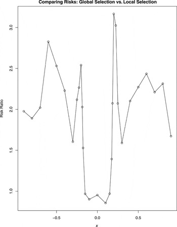
. The results are presented in Figure 2 at a number of x0 values in the range of (−1,1).

Risk ratio of a global CV vs. a nonglobal selection method.
The figure clearly shows that the nonglobal selection performs much better than the global selection except in a very small neighborhood around zero, demonstrating the potentially great advantage of considering nonglobal selection among candidate procedures.
It is probably fair to say that one may not necessarily choose the form of

from inspecting the scatter plot. In Section 2.2, we use logistic regression to find the preference region automatically.
2.2. Classification for Estimating the Preference Region
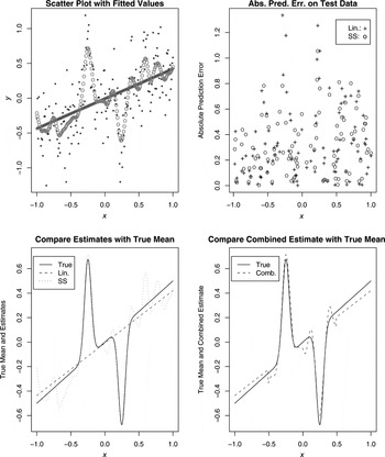
We continue with the earlier setting except that the sample size is now 200 (so that the contrast is more clearly seen in the next figure). We focus on one typical realization of the data. A scatter plot of the data with the linear and the SS fits is given in the upper left panel of Figure 3. We use logistic regression as the classification method to find the region where the linear estimator performs better than the SS estimator. With a random splitting of the data into two parts of equal size, we fit a straight-line model and the SS using the first 100 observations and obtain the binary variable that indicates which method has a smaller prediction error on the second 100 observations. A typical outcome is in the upper right panel of Figure 3. One may get the impression that SS tends to do better in the middle and less well at the ends. We fit a logistic regression model with three terms: 1, x, and x2. The estimated probability that the linear model performs better at x is

Note that

corresponds to x < (−0.51) or x > 0.49, which is very sensible judging from our knowledge of the true mean function (despite that the upper right panel of the figure does not seem to be very visually informative for relating the relative performance of the two estimators and x). This yields the following combined estimate of the regression function:

where

and

are the linear and SS estimates of f based on the full data. This estimate is compared with the true function in the lower right panel of Figure 3.

An example of using logistic regression for nonglobal selection.
From the lower left panel of Figure 3, we see that the linear estimate is very poor around −0.25 and 0.25 (not surprisingly); in contrast, the SS estimate is quite good there, but it pays a price for being flexible in terms of accuracy at other locations. Globally, the SS is much better than the linear estimate. Indeed, the ratio of their integrated squared errors is over 6.23. Thus from the global perspective, the SS estimate is the clear winner. However, with the use of logistic regression, we properly figured out that when x is far away from zero by a certain degree, the linear estimate is better. Although the linear estimate is slightly biased even in the linear parts, its use in the final combined estimate is very helpful as seen in the figure. Numerically, the integrated squared error of the combined estimate is only 35% of that of the SS estimate. Therefore a globally poor method can still make a good contribution if it is properly combined with a globally much better estimator.
3. THREE APPROACHES TO NONGLOBAL MODEL SELECTION
Consider two procedures δ1 and δ2 with risks R(δ1;x;n) and R(δ2;x;n) at a given x value based on a sample of size n. Let A* = {x : R(δ1;x;n) ≤ R(δ2;x;n)} be the set of x at which the first procedure performs no worse than the second one. It is the preference region of δ1 (relative to δ2). Ideally, for selection, one would use δ1 on A* and δ2 on (A*)c. In reality, one may have little prior knowledge of the form of A*, and to deal with the issue, one may consider graphical inspections when x is of a low dimension or consider A from a class of sets with proper complexity in the hope that one member is close to A*. One can consider various sets of A of different degrees of locality. We consider three approaches here.
3.1. Neighborhood-Based Selection
Instead of directly estimating A*, at each given x0, one considers a local neighborhood around x0 and tries to find the candidate that performs better in the local area. This approach can be very helpful when A* cannot be described well by simple sets. It will be studied in detail in Section 4.
3.2. Empirical Risk Minimization
One considers a collection of sets of a certain mathematical form and tries to identify the one with the best performance. Here the collection may depend on the sample size. The size of the collection can be predetermined or adaptively chosen. This approach will be explored briefly in Section 5.
3.3. Classification-Based Selection
Sometimes, one is less confident to go with any specific collection of sets as the preference region. This is especially true when the input dimension is high, where neighborhood-based selection may perform poorly because of the curse of dimensionality. In such a case, one can take advantage of classification methods to conduct localized selection as in Section 2.2. In general, one splits the data into two parts. The first part is used to obtain the estimates from the candidate procedures and then to make predictions for the second part. Based on the relative predictive performance in each case, we create a new variable that simply indicates which estimate is the better one. Then we can apply a sensible classification method to relate the performance indication variable to the covariates. If a classifier performs well, it indicates that the candidate procedures' relative performance depends on the covariates, and we can do better than globally selecting one of the procedures.
4. LOCALIZED CROSS VALIDATION SELECTION
CV (see, e.g., Allen, 1974; Stone, 1974; Geisser, 1975) has been widely used for model selection. In this section, we consider a localized CV method for selecting a candidate procedure locally. For a given x0, consider the ball centered at x0 with radius rn for some rn > 0 under the euclidean distance. We randomly split the data into a training set of size n1 and a test set of size n2, and then we use the training set to do estimation by each regression procedure. For evaluation, consider only the data points in the test set that are in the given neighborhood of x0. Let

be the procedure that has the smaller average squared prediction error. This process is repeated with a number of random splittings of the observations to avoid the splitting bias. The procedure that wins more frequently over the permutations is the final winner. We call this a localized cross validation (L-CV) at x0 of rn-neighborhood.
For the local selection problem, we are interested in the question of under which conditions the locally better estimator will be selected with high probability. More precisely, assuming that when n is large enough, one procedure has risk at x0 smaller than that of the other one, we want to select the better one with probability approaching 1. If a selection method has this property, we say it is locally consistent in selection at x0. For related results on global CV, see, e.g., Li (1987), Burman (1989), Zhang (1993), Shao (1997), Wegkamp (2003), and Yang (2007).
Given x0 and η > 0, let

be a local loss of an estimate

around x0, where

denotes the distribution of X conditional on that X takes value in the neighborhood B(x0;η). Let ∥·∥s,x0;η denote the Ls norm around x0 with radius η, i.e.,

.
DEFINITION 1. Procedure δ1 (or

) is asymptotically better than δ2 (or

) under the squared loss at ηn-neighborhood of x0, denoted δ1 [ltri ] δ2 at (x0;ηn), if for each nonincreasing sequence

with

and every 0 < ε < 1, there exists a constant cε > 0 such that when n is large enough,

When one of the procedures is asymptotically better than the other at a neighborhood of x0, we say that δ1 and δ2 are ordered at x0. One may wonder if it is better to require the condition in (1) for ηn only. The answer is no because it is possible that

is smaller than

with high probability for one sequence of ηn yet the opposite holds for a smaller sequence 0 < ηn′ ≤ ηn. This can happen, e.g., when δ1 is asymptotically better than δ2 globally (i.e., with no restriction on ηn) but worse locally. In general, the space

can be decomposed into three regions: those x0 at which δ1 is asymptotically better than δ2, those at which δ2 is asymptotically better than δ1, and the rest of x0 at which δ1 and δ2 cannot be compared according to Definition 1. Local selection can be hoped to be successful only for the first two regions.
DEFINITION 2. A procedure δ (or

) is said to converge exactly at rate {an} in probability at ηn-neighborhood of x0 if for each nonincreasing sequence

with

,

, and for every 0 < ε < 1, there exists cε > 0 such that when n is large enough,

.
DEFINITION 3. A selection method is said to be locally consistent in selection at x0 if δ1 and δ2 are ordered at x0 and the asymptotically better procedure at x0 is selected with probability going to 1. If the selection method is locally consistent at every x0 at which the procedures are ordered, it is said to be locally consistent.
In Definition 2, the second condition simply indicates that the loss does not converge faster than an in an appropriate sense. For the following result, we assume that

and

converge exactly at rate {pn} and {qn} in probability at ηn-neighborhood of x0, respectively, where pn and qn are two sequences of nonincreasing positive numbers.
Some technical conditions are needed.
Condition 1. There exists a sequence of positive numbers An such that for j = 1,2,

Condition 2. There exists ηn > 0 such that δ1 [ltri ] δ2 at (x0;ηn) or δ2 [ltri ] δ1 at (x0;ηn). Let j*(x0) denote the better procedure.
Condition 3. There exists a sequence of positive numbers {Mn} such that for j = 1,2, for each nonincreasing sequence

, we have

THEOREM 1. Under Conditions 1–3, as long as n1, n2, and rn are chosen to satisfy (1): n2rndMn1−4 → ∞; (2)

; (3) rn ≤ ηn, we have that with probability going to 1, the better procedure

will be selected.
From the result, several factors affect the ability of the L-CV to identify the best estimator at a given x0. The larger ηn, the larger the window for choosing the neighbor size rn for L-CV. Intuitively, if ηn is very close to zero, which occurs when the two procedures constantly switch position in terms of local performance, it may not be feasible to identify the locally better one at all. The constants Mn and An come into the picture more for a technical reason. For simplicity, for the following discussion, we assume that Mn and An are both of order 1. Then the requirements on the choice of data splitting ratio and the neighbor size become

and rn ≤ ηn. Consider, e.g., ηn = (log n)−1. When at least one of the procedures is nonparametric with max(pn,qn) converging more slowly than the parametric rate n−1/2, Yang (2007) showed that for selecting the globally better procedure, it suffices to take n2 at least of the same order as n1 (which is not enough for comparing parametric models as shown in Shao, 1993). With local selection, however, we need to be more careful so as to satisfy

If max(pn,qn) is of order n−1/3, then with n1 = n2, the condition is simply n−1/(3d) << rn ≤ (log n1)−1.
When the number of observations is moderately large, one can use a data dependent approach to choose rn. For example, taking rn to be the same for all x, one may consider another level of data splitting for empirically evaluating the performance of each choice of rn. Theoretical results are possible, but we will not pursue them in this work.
5. PREFERENCE REGION SELECTION
Let

and

be the estimates by the two regression procedures based on the first part of the data of size n1. For a measurable set A, define

Because

it follows that the preference region

is the best choice of A. Obviously, we have

i.e., if it is possible to identify A*, the estimator

is better (or at least no worse) than the global winner between the two candidate procedures. The ideal local selection can be arbitrarily better than the global selection in terms of their risk ratio.
We consider a collection of sets of manageable complexity and try to find the best set A within the class. Let

be a class of sets and let An* be the set that minimizes

over

. Then

is the approximation error because of the use of a set in

, which may not contain A*. Of course, An* is also unknown and needs to be estimated.
Let μ(B [utri ] A) denote the probability (under the distribution of Xi) of the symmetric difference of A and B. Assume that

has metric entropy bounded above by Hn(ε) under the distance d(A,B) = μ(B [utri ] A) (for concept and related results involving metric entropy, see, e.g., Kolmogorov and Tihomirov, 1959; Yatracos, 1985; Birgé, 1986; van de Geer, 1993; Yang and Barron, 1999). Let

be a discretized collection of sets that serves as an εn-net for

under d. Let

be the minimizer of the empirical prediction error over

, i.e.,

THEOREM 2. Assume that the errors are normally distributed with mean zero and variance σ2 > 0 and

for some constant C < ∞ for both procedures. Then the final estimator

satisfies

where the constants C1 and C2 depend only on C and σ2.
To optimize the risk bound given previously, with

given, we need to balance (Hn(εn))/n2 and εn. The issue becomes more complicated when one needs to choose

. Clearly, a large choice of

reduces the potential approximation error but at the same time increases the estimation error because of searching over a larger class of sets A. One approach to handling the approximation error is to assume that A* is in a given collection of sets

and then to characterize the uniform approximation error of sets in

by sets in

. Define

. Under proper assumptions on

and

, the rate of convergence of γn can be derived and then used for obtaining the convergence rate of the final estimator from the localized selection.
Example
Let

consist of all possible unions of at most k cubes in

. Let

be the collection of all the sets that each can be well approximated by a set in

in the sense that for each

, there exists a set A in

such that μ(B [utri ] A) ≤ ck−τ for some constants c,τ > 0. For simplicity, we assume that Xi has a uniform distribution on [0,1]d, although a similar result holds if Xi has a uniformly upper bounded Lebesgue density.
To obtain an ε-net in

for

, we first choose k = kε such that ck−τ ≤ ε/2 (kε is then of order ε−1/τ). Then for any

, there exists a set A in

such that μ(B [utri ] A) ≤ ε/2. Consequently, an ε/2-net in

will be an ε-net for

. Now if we have a grid on [0,1]d of width ε/(2k) for each coordinate, then the collection of all cubes with vertices on the grid form an ε/(2k)-net for

and thus also an ε-net for

. The number of possible unions of k such cubes is of order

It follows that the metric entropy of

is of order O(ε−1/τ log(ε−1)).
If we select A over the ε-net in

by CV with a proper discretization, by Theorem 2, with a choice of n1 and n2 both of order n, the combined estimator satisfies

Balancing the last two terms in the preceding expression, the optimal choice of εn is (log n/n)τ/(τ+1), and consequently the risk bound becomes

Thus, when τ is large, the additional term (log n/n)τ/(τ+1) is close to log n/n, which is typically negligible for nonparametric regression. Then we achieve the performance of the ideal localized selection up to a relatively small discrepancy term.
6. CONCLUDING REMARKS
Overall performance of a candidate model (procedure) has been the dominating measure used for model selection. If one candidate model is thought to be “true” or “optimal,” it is then rational to try to identify it. However, in many applications, this practice is suboptimal because the globally best candidate procedure, even if it is much better than others, may still have unsatisfactory local behaviors in certain regions, which can be remedied well with helps from other candidates that are globally inferior.
We took two directions in localized model selection: a localized CV that selects a model/procedure at each x value based on performance assessment in a neighborhood of x and a preference region selection from a collection of sets that tries to estimate the regions where each candidate performs better. For the localized CV, as long as the neighborhood size and the data splitting ratio are chosen properly, the locally better estimator will be selected with high probability. For preference region selection, when the complexity of the collection of the candidate sets of the preference region is properly controlled, the final procedure based on the empirically selected preference region behaves well in risk.
Besides global selection and localized selection of a model, sometimes it is advantageous to consider global combination of the candidates with weights globally determined or localized combination where weights depend on the x value (see, e.g., Pan, Xiao, and Huang, 2006). For high-dimensional or complex data, these alternatives can provide flexibility needed to further improve performance of the candidate procedures.
APPENDIX
Proof of Theorem 1. Much of the proof follows from Yang (2007), except that localized selection is considered in this work. We first focus on the analysis without multiple data splittings. Without loss of generality, assume that δ1 is asymptotically better than δ2 at x0. Let I = Ix0,rn = {i : n1 + 1 ≤ i ≤ n and Xi ∈ B(x0;rn)} denote the observations in the evaluation set with Xi close to x0 and let

be the size of I. Because


is equivalent to

Conditional on Z1 = (Xi,Yi)i=1n1 and X2 = (Xn1+1,…,Xn), assuming

is larger than

, by Chebyshev's inequality, we have

Let Qn denote the ratio in the upper bound in the preceding inequality and let Sn be the event of

Then because

for consistency, it suffices to show that P(Snc) → 0 and Qn → 0 in probability. Suppose we can show that for each ε > 0, there exists αε > 0 such that when n is large enough,

Then P(Sn) ≥ 1 − ε and thus P(Snc) → 0 as n → ∞. Because

with probability no less than 1 − ε, we have

From (A.1) and (A.2), to show P(Snc) → 0 and Qn → 0 in probability, it suffices to show (A.1) and

Suppose a slight relaxation of Condition 1 holds: for every ε > 0, there exists An1,ε such that for j = 1,2, when n1 is large enough,

Let Hn1 denote the event

. Then on Hn1, we have

with Xi ∈ B(x0;rn) is bounded between −(An1,ε)2 and (An1,ε)2. Conditional on Z1 and Hn1,

, where the subscript Z1 in VarZ1 and EZ1 is used to denote the conditional expectation given Z1. Thus conditional on Z1, on Hn1, by Bernstein's inequality (see, e.g., Pollard, 1984, p. 193), for each x > 0,

Taking

, the preceding inequality becomes

Under Condition 2, for every ε > 0, there exists αε′ > 0 such that when n is large enough,

Take βn such that

Then with probability at least 1 − ε, βn ≥ (αε′/2)/(1 + αε′/2). Let Dn denote this event. Then on Dn, we have

and

If we have


then the upper bound in the last inequality in the expression preceding (A.4) converges to zero in probability. From these pieces, we can conclude that

for some Δ(ε,n) → 0 as n → ∞. Indeed, for every given ε > 0, when n is large enough,

where the expectation in the upper bound of the last inequality (i.e., Δ(ε,n)) converges to zero because of the convergence in probability to zero of the random variables of the exponential expression and their uniform integrability (because they are bounded above by 1), provided that (A.4) and (A.5) hold. The assertion of (A.6) then follows.
For the other estimator, similarly, for

, we have

If we have


then following a similar argument used for

, we have

From this, if

in probability and

is bounded away from 1, then (A.3) holds. If in addition, we can choose

, then for each given ε, we have

for some small αε > 0 when n1 is large enough. Now for every

, we can find ε > 0 such that

and there exists an integer n0 such that when n ≥ n0 the probability in (A.9) is upper bounded by

and

. Consequently when n ≥ n0,

Recall that we needed the conditions (A.4), (A.5), (A.7), and (A.8) for (A.1) to hold. Under Condition 3,

is lower bounded in order in probability by

. From all that precedes, because

and

converge exactly at rates pn and qn, respectively, under the L2 loss, we know that for the conclusion of Theorem 1 to hold, it suffices to have the following requirements: for every ε > 0, for some

,


Note that

is a random variable that has a binomial distribution with n2 trials and success probability P(Xi ∈ B(x0;rn)). Under the assumption that the density of X is bounded away from zero in a neighborhood of x0, P(Xi ∈ B(x0;rn)) is of order rnd. We need to lower bound

in probability. For 1 ≤ j ≤ n2, let Dj be independent Bernoulli random variables with success probability β. Then applying Bernstein's inequality (see, e.g., Pollard, 1984, p. 193), we have

For our setting, β is of order rnd. Thus

is at least of order n2rnd in probability if n2rnd → ∞. Consequently, the earlier requirements on the splitting ratio become that for every ε > 0, for some

,


Under Condition 1, for every ε > 0, there exists a constant Bε > 0 such that

when n1 is large enough. That is, for a given ε > 0, we can take An1,ε = O(An1). Therefore if we have n2rndMn1−4 → ∞ and n2rndqn12/(1 + An1) → ∞, then we can find

such that the preceding five displayed requirements are all satisfied.
Let π denote a permutation of the observations and let Π denote a set of such permutations. Let

be the L-CV criterion value under the permutation π. If

, then let τπ = 1 and otherwise let τπ = 0. Let W denote the values of (X1,Y1),…,(Xn,Yn) (ignoring the orders). Under the i.i.d. assumption on the observations, obviously, conditional on W, every ordering of these values has exactly the same probability, and thus

From the earlier analysis, we know that

. Thus E([sum ]π∈Πτπ/|Π|) → 1. Because [sum ]π∈Πτπ/|Π| is between 0 and 1, for its expectation to converge to 1, we must have [sum ]π∈Πτπ/|Π| → 1 in probability. This completes the proof of Theorem 1. █
Proof of Theorem 2. Let

be the minimizer of E∥f(;A) − f∥2 over

. By the results of Wegkamp (2003, Sect. 2), in particular Theorem 2.1, we have

where B1 and B2 are constants that depend only on C and σ2.
Note that

Together with

being an εn-net under d, we have

. The conclusions then follow. This completes the proof of Theorem 2. █