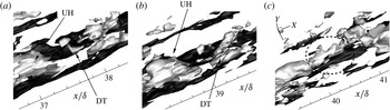
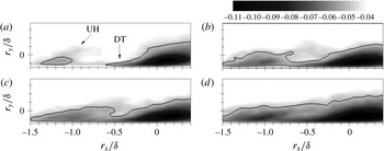
1 Introduction
For several decades, the study of zero pressure gradient (ZPG) turbulent boundary layer (TBL) flows has been performed extensively for engineering applications, as boundary layers are present wherever there is a fluid flow over a wall. However, much less is known with regard to TBL flows subjected to adverse pressure gradients (APGs), although these flows are easily observed in actual engineering applications, including diffusers, turbine blades and the trailing edges of airfoils. In particular, because large-scale structures play a crucial role in the generation of the turbulent production and transport of wall turbulence, an understanding of the APG effects on large-scale features in TBL flows will contribute to further advances in the development of effective flow control methods which are applicable while also increasing the accuracy of turbulence modelling for predictions.
Many important features of turbulent statistics in equilibrium APG TBL flows have been clarified thus far. In general, as the magnitude of an APG increases, the mean velocity profile develops a large wake region (Harun et al.
Reference Harun, Monty, Mathis and Marusic2013). In addition, the log region of the mean velocity profile is shifted below the standard log law profile in a ZPG TBL flow (Nagano, Tagawa & Tsuji Reference Nagano, Tagawa, Tsuji, Durst, Friedrich, Launder, Schmidt, Schumann and Whitelaw1993; Na & Moin Reference Na and Moin1998). Lee & Sung (Reference Lee and Sung2008) showed that the root mean square of velocity fluctuations and Reynolds shear stresses in APG flows are increased in the outer layer due to an enhancement of the outer vortical structures, consistent with a direct numerical simulation (DNS) study by Skote, Henkes & Henningson (Reference Skote, Henkes and Henningson1998) for APG TBL flows. In addition, a Reynolds stress budget analysis revealed that the energy redistribution from streamwise to wall-normal and spanwise velocity components is intensified in the outer layer of APG flows (Lee & Sung Reference Lee and Sung2008), and the dominant secondary peak of the production term occurs at the half height of the boundary layer thickness
 $\unicode[STIX]{x1D6FF}$
approximately (Skåre & Krogstad Reference Skåre and Krogstad1994). Harun et al. (Reference Harun, Monty, Mathis and Marusic2013) analysed the production of turbulent energy and showed that the combination of mean shear and large-scale activity of structures increases the streamwise turbulence intensity in the outer layer. The inward turbulent energy transport in an APG flow, which is opposite to that under a ZPG flow, was found near the log region (Lee & Sung Reference Lee and Sung2008).
Given that large-scale motions, which are found to scale on the boundary layer thickness with average dimensions greater than
 $1\unicode[STIX]{x1D6FF}$
(in terms of the length), make dominant contributions to generate streamwise turbulent kinetic energy and Reynolds shear stress in the outer layer in wall-bounded turbulent flows (Wu, Baltzer & Adrian Reference Wu, Baltzer and Adrian2012), the structural organizations of the outer regions of large-scale structures in APG TBLs have been actively examined (Krogstad & Skåre Reference Krogstad and Skåre1995; Lee & Sung Reference Lee and Sung2009; Monty, Harun & Marusic Reference Monty, Harun and Marusic2011; Rahgozar & Maciel Reference Rahgozar and Maciel2011; Harun et al.
Reference Harun, Monty, Mathis and Marusic2013). In an experimental study of APG TBLs, Krogstad & Skåre (Reference Krogstad and Skåre1995) calculated two-point spatial correlations in the log layer using arrays of eight equally spaced X-wire probes. They showed that streamwise length scales based on correlation contours are reduced when an APG is applied to a TBL flow, whereas spanwise length scales are increased within the log layer. Similar results were reported by Rahgozar & Maciel (Reference Rahgozar and Maciel2011) through a particle image velocimetry experiment in an APG TBL. They found long meandering regions of the streamwise velocity-fluctuating structures at the top of the log layer (and above) of an APG flow, similar to a ZPG TBL flow (Hutchins & Marusic Reference Hutchins and Marusic2007a
), while these structures are observed less frequently in an APG flow than in a canonical ZPG flow.
In contrast, a recent experimental study by Harun et al. (Reference Harun, Monty, Mathis and Marusic2013) showed that the long-wavelength energy in the two-dimensional premultiplied streamwise energy spectra is more amplified in an entire equilibrium APG boundary layer compared with that in a ZPG flow, although the overall shapes of the two spectrum maps are similar. Based on these findings, they suggested that the APG either strengthens the outer-region large-scale structures or induces a large number of large-scale motions in the outer layer. In addition, Monty et al. (Reference Monty, Harun and Marusic2011) found using decomposed turbulent intensity profiles that the intensification of large-scale motions is essential to increase the streamwise turbulent intensity through the wall layer in APG flows. Further evidence of greater large-scale turbulence activity is provided in a DNS study of APG TBL flows by Lee & Sung (Reference Lee and Sung2009). Based on wall-normal variations of streamwise lengths extracted from two-point correlations of streamwise velocity fluctuations, they showed that the streamwise and spanwise length scales are larger for an APG flow than for a ZPG flow within the log layer (
 $y/\unicode[STIX]{x1D6FF}<0.2$
). Lee & Sung (Reference Lee and Sung2009) attributed the increased length scales to the intensified and regulated low-momentum regions in the outer layer caused by APGs using a conditionally averaged flow field with a spanwise swirling event. Harun et al. (Reference Harun, Monty, Mathis and Marusic2013) explained that the different nature of the large-scale structure relative to that identified by Krogstad & Skåre (Reference Krogstad and Skåre1995) could be due to incomplete inferences based on superimposed contour lines of the two-point correlations.
Although there is less consensus regarding the influence of APGs on the outer-region large-scale structures in TBL flows, a careful review of the literature as given above shows that the strength of the APG, e.g. the non-dimensional pressure gradient parameter
 $\unicode[STIX]{x1D6FD}$
, defined as
 $\unicode[STIX]{x1D6FF}^{\ast }/\unicode[STIX]{x1D70F}_{w}(\text{d}P/\text{d}x)$
, may be important in determining the large-scale features in the outer layer, where
 $\unicode[STIX]{x1D6FF}^{\ast }$
is the displacement thickness,
 $\unicode[STIX]{x1D70F}_{w}$
is the wall-shear stress and
 $\text{d}P/\text{d}x$
is the mean pressure gradient in the streamwise direction. If
 $\unicode[STIX]{x1D6FD}$
is sufficiently large, e.g.
 $\unicode[STIX]{x1D6FD}=20$
(Krogstad & Skåre Reference Krogstad and Skåre1995) and
 $\unicode[STIX]{x1D6FD}=8.5{-}244.6$
(Rahgozar & Maciel Reference Rahgozar and Maciel2011), the streamwise lengths of the large-scale motions are shortened by the APG, whereas they are more energized with longer streamwise coherence for relatively small values of
 $\unicode[STIX]{x1D6FD}$
, e.g.
 $\unicode[STIX]{x1D6FD}=1.74$
(Harun et al.
Reference Harun, Monty, Mathis and Marusic2013),
 $\unicode[STIX]{x1D6FD}=0.82{-}4.74$
(Monty et al.
Reference Monty, Harun and Marusic2011) and
 $\unicode[STIX]{x1D6FD}=1.68$
(Lee & Sung Reference Lee and Sung2009).
In the present study, DNS of spatially developing TBLs under a wide range of APG strengths are performed in order to provide a clear picture of the relationship between an APG and the large-scale features in the outer layer. Because it is well known that the largest structures in a ZPG TBL flow are frequently observed in the log region with high low-wavenumber energy (Hutchins & Marusic Reference Hutchins and Marusic2007a ), special attention is given to structural modifications of the log region large-scale features by APGs. The effects of APGs on the large-scale structures in the log layer are documented based on an analysis of the instantaneous flow fields, two-point correlations, energy spectrum maps and the two-point amplitude modulation effect. In order to identify the spatial organization of conditional structures associated with the spanwise-oriented vortex and second- and fourth-quadrant Reynolds shear stresses in a mean sense, linear stochastic estimation (LSE), which is based on the two-point correlation tensor of the velocity fluctuations, is employed. The identified conditional structures provide the basis of an explanation of the distinct streamwise length scales of the log region large-scale structures under APGs. Finally, time-resolved instantaneous flow fields are analysed to show the streamwise scale growth of the large-scale structures in the log layer by merging events in a mild APG TBL flow.
2 Computational details
For an incompressible flow, the non-dimensional governing equations are
 $$\begin{eqnarray}\displaystyle & \displaystyle \frac{\unicode[STIX]{x2202}u_{i}}{\unicode[STIX]{x2202}dt}+\frac{\unicode[STIX]{x2202}u_{i}u_{j}}{\unicode[STIX]{x2202}x_{j}}=-\frac{\unicode[STIX]{x2202}p}{\unicode[STIX]{x2202}x_{i}}+\frac{1}{Re}\frac{\unicode[STIX]{x2202}^{2}u_{i}}{\unicode[STIX]{x2202}x_{j}\unicode[STIX]{x2202}x_{j}}, & \displaystyle\end{eqnarray}$$
 $$\begin{eqnarray}\displaystyle & \displaystyle \frac{\unicode[STIX]{x2202}u_{i}}{\unicode[STIX]{x2202}x_{i}}=0, & \displaystyle\end{eqnarray}$$
 $x_{i}$
denotes the Cartesian coordinates and
 $u_{i}$
represents the corresponding velocity components. All variables are non-dimensionalized by the inlet free-stream velocity (
 $U_{0}$
) and the inlet momentum thickness (
 $\unicode[STIX]{x1D703}_{in}$
), and the inlet Reynolds number is defined as
 $Re=U_{0}\unicode[STIX]{x1D703}_{in}/\unicode[STIX]{x1D708}$
, where
 $\unicode[STIX]{x1D708}$
is the kinematic viscosity. The equations are integrated in time using the fractional step method along with the implicit velocity decoupling procedure (Kim, Baek & Sung Reference Kim, Baek and Sung2002). A block LU (lower upper) decomposition based on approximate factorization is applied to achieve both velocity–pressure decoupling and the decoupling of intermediate-velocity components. In this approach, the terms are first discretized in time using the Crank–Nicholson method, and then the coupled velocity components are solved without iteration. All terms are resolved using a second-order central difference scheme in space with a staggered mesh. The numerical scheme used in the present work is identical to that of Lee & Sung (Reference Lee and Sung2009).
The notation adopted is such that
 $x$
,
 $y$
and
 $z$
denote the streamwise, wall-normal and spanwise coordinates respectively, while
 $u$
,
 $v$
and
 $w$
denote the corresponding velocity components. In order to provide the effects of APGs in TBL flows, the free-stream velocity
 $U_{\infty }$
at the top boundary of the rectangular computational domain is specified along the streamwise direction as follows (Mellor & Gibson Reference Mellor and Gibson1966):
 $$\begin{eqnarray}\displaystyle \left.\begin{array}{@{}c@{}}u=U_{\infty }(x)=\left\{\begin{array}{@{}ll@{}}U_{0},\quad & \text{for }x<0,\\ U_{0}\left(1-\displaystyle \frac{x}{x_{0}}\right)^{m},\quad & \text{for }x\geqslant 0,\end{array}\right.\\ \displaystyle \frac{\unicode[STIX]{x2202}v}{\unicode[STIX]{x2202}y}=-\frac{\unicode[STIX]{x2202}u}{\unicode[STIX]{x2202}y},\\ \displaystyle \frac{\unicode[STIX]{x2202}w}{\unicode[STIX]{x2202}y}=0,\end{array}\right\} & & \displaystyle\end{eqnarray}$$
where
 $m$
denotes the exponent of the APG and
 $x_{0}$
indicates the streamwise distance from the inlet at which the APG is applied (
 $x_{0}/\unicode[STIX]{x1D703}_{in}=300$
). In the present study, four different values of
 $m$
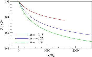
are considered (figure 1), namely
 $m=0$
,
 $-$
0.15,
 $-$
0.25 and
 $-$
0.32. The corresponding computational domain size and mesh resolution are summarized in table 1. All of the computational conditions are identical regardless of
 $m$
to eliminate any influence on our results, except for the domain size. Although not shown here, a grid sensitivity study with doubled and quadruple resolutions for computational feasibility indicated that the influence of the mesh resolution is negligible on first-, second- and higher-order statistics in the simulations for all values of
 $m$
. The streamwise domain size is sufficiently long to reach a new equilibrium state under the APGs from a ZPG flow, and the streamwise domain size normalized by the inlet boundary layer thickness is 320 for ZPG and mild APG flows and 480 for moderate and strong APG flows. The streamwise domain sizes for the equilibrium regions of APG flows are more than 15–20 times the boundary layer thickness at the outlet; thus, the streamwise lengths are sufficient to capture large-scale structures with a mean wavelength of up to
 $8{-}20\unicode[STIX]{x1D6FF}$
based on previous observations of ZPG TBL flows (Balakumar & Adrian Reference Balakumar and Adrian2007; Hutchins & Marusic Reference Hutchins and Marusic2007a
; Lee & Sung Reference Lee and Sung2011). It should also be noted that the computational domain size in the streamwise direction is longer than that in Lee & Sung (Reference Lee and Sung2009) to examine the modification of large-scale structures in a stable equilibrium state in the downstream region. The streamwise resolution is comparable to those employed in previous DNS studies of APG TBLs:
 $\unicode[STIX]{x0394}x^{+}=13$
(Skote et al.
Reference Skote, Henkes and Henningson1998) and
 $\unicode[STIX]{x0394}x^{+}=16.6$
(Na & Moin Reference Na and Moin1998). A no-slip boundary condition is imposed at the solid wall, and periodic boundary conditions are applied in the spanwise direction. An auxiliary simulation for the inlet boundary condition for a ZPG TBL flow is carried out based on the method of Lund, Wu & Squires (Reference Lund, Wu and Squires1998) at
 $Re_{\unicode[STIX]{x1D703}}=300$
. Although not shown here, a direct comparison of the mean velocity and turbulent intensity profiles with DNS data from Spalart (Reference Spalart1988) shows excellent agreement. The convective boundary condition at the exit is specified as
 $(\unicode[STIX]{x2202}u/\unicode[STIX]{x2202}t)+c(\unicode[STIX]{x2202}u/\unicode[STIX]{x2202}x)=0$
, where
 $c$
is the local bulk velocity. Non-uniform grid distributions are employed in the wall-normal direction using a hyperbolic tangent function and a uniform grid distribution in both the streamwise and spanwise directions.
Free-stream velocity distributions for four different values of
 $m$
along the upper boundary of the computational domain. For
 $m=0$
,
 $U_{\infty }/U_{0}=1$
.

Domain size and mesh resolution.

In our simulations, the initial velocity condition is imposed by the Blasius laminar velocity profile, and a turbulent flow obtained from an inflow simulation is imposed in time at the inlet. During the transient process, the upper boundary condition is maintained as
 $U_{\infty }/U_{0}=1.0$
(that is, a ZPG TBL flow). After the flow reaches a fully turbulent flow through the entire domain, four different conditions for the top boundary are utilized to simulate the ZPG and APG TBL flows (
 $-0.32\leqslant m\leqslant 0$
). Statistical quantities are obtained from temporal and spatial averaging only in the spanwise direction when the APG flows are fully developed through the entire domain, and total averaging is conducted during
 $48\,000\unicode[STIX]{x1D703}_{in}/U_{0}$
, which corresponds to 16 sweeps across the entire bulk flow domain. A total of 1900 instantaneous realizations are collected with a time interval of
 $32\unicode[STIX]{x1D703}_{in}/U_{0}$
. A superscript
 $+$
indicates quantities normalized by the local mean friction velocity (
 $u_{\unicode[STIX]{x1D70F}}$
) and a capital letter or bracket
 $\langle \cdot \rangle$
indicates temporally and spatially averaged statistics. The prime indicates fluctuating quantities; e.g.,
 $u^{\prime }$
is the streamwise velocity fluctuation. In order to divide large-scale and small-scale signals from the raw velocity fluctuations, spectral decomposition of the velocity fluctuations is performed based on a cutoff wavelength of
 $\unicode[STIX]{x1D706}_{z}/\unicode[STIX]{x1D6FF}=0.5$
(where
 $\unicode[STIX]{x1D706}_{z}$
is the spanwise wavelength) according to the method suggested by Bernardini & Pirozzoli (Reference Bernardini and Pirozzoli2011). Because boundary layer flows develop spatially in the streamwise direction, it is not possible to compute the Fourier modes of the signal in the streamwise direction. However, because large spanwise structures are closely associated with large streamwise structures on average (Tomkins & Adrian Reference Tomkins and Adrian2003), the spatial features of large-scale streamwise structures detected based on the spanwise cutoff wavelength are expected to be similar to those from the streamwise cutoff wavelength. In addition, although the effect of varying the filter width is preliminarily addressed, no qualitative difference is observed.
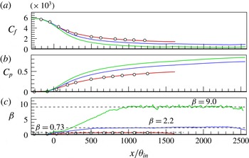
Streamwise variation of (a) the skin-friction coefficient
 $C_{f}$
, (b) the pressure coefficient
 $C_{p}$
and (c) the non-dimensional pressure gradient parameter
 $\unicode[STIX]{x1D6FD}$
for
 $m=0$
,
 $-$
0.15,
 $-$
0.25 and
 $-$
0.32. The circle symbols indicate DNS data from Lee & Sung (Reference Lee and Sung2009) with
 $m=-0.15$
. In (c), the three dashed lines depict
 $\unicode[STIX]{x1D6FD}$
values of 0.73, 2.2 and 9.0. The line legend is identical to that in figure 1.

3 Results and discussion
3.1 Turbulent statistics
Before analysing the modification of large-scale features by APGs, it is necessary not only to check the reliability and accuracy of the numerical simulations but also to examine whether new equilibrium states are established under APGs. Figure 2(a,b) shows the streamwise variation of the skin-friction coefficient
 $C_{f}$
and pressure coefficient
 $C_{p}$
as the APG strength
 $m$
varies. A comparison of our results with earlier DNS data from Lee & Sung (Reference Lee and Sung2009) with an identical value of
 $m$
 $(=-0.15)$
exhibits excellent agreement along the streamwise direction. For each
 $m$
, the boundary layer flow near the inlet (
 $x/\unicode[STIX]{x1D703}_{in}<0$
) develops under a ZPG (
 $\text{d}C_{p}/\text{d}x=0$
), after which the streamwise pressure gradient is applied along the downstream direction, leading to a significant decrease of
 $C_{f}$
and an increase of
 $C_{p}$
due to
 $\text{d}P/\text{d}x>0$
. The changes in
 $C_{f}$
and
 $C_{p}$
are greater as the pressure gradient increases, and
 $C_{f}$
and
 $C_{p}$
vary monotonically as the flows move further downstream. The non-dimensional pressure gradient parameter
 $\unicode[STIX]{x1D6FD}$
is shown in figure 2(c). It is clear for all
 $m$
that
 $\unicode[STIX]{x1D6FD}$
converges to a constant value after a continuous increase in the initial stage, showing that self-preservation is achieved within the computational domain. Because the computational domain near the outlet is contaminated by the outflow in all cases, the streamwise extent for
 $(100{-}200)\unicode[STIX]{x1D703}_{in}$
near the outlet must be discarded. As
 $m$
increases, the strength of the APGs increases dramatically, causing
 $\unicode[STIX]{x1D6FD}$
to vary in the range of
 $0.73\leqslant \unicode[STIX]{x1D6FD}\leqslant 9.0$
in the equilibrium regions. These values of
 $\unicode[STIX]{x1D6FD}$
cover mild, moderate and strong APGs, and distinct large-scale features of the velocity organization are expected, as stated in the introduction. It should be noted that although the minimum value of
 $C_{f}$
(
 $=5.0\times 10^{-4}$
) when
 $m=-0.32$
is comparable to the value (
 $=5.7\times 10^{-4}$
) in Krogstad & Skåre (Reference Krogstad and Skåre1995),
 $\unicode[STIX]{x1D6FD}$
is significantly smaller in the present study than
 $\unicode[STIX]{x1D6FD}=20$
in Krogstad & Skåre (Reference Krogstad and Skåre1995). Our additional simulation with a higher
 $m$
to match
 $\unicode[STIX]{x1D6FD}$
suggests that as
 $\unicode[STIX]{x1D6FD}$
increases further, the flow becomes very unstable due to flow separation. In addition, although Mellor & Gibson (Reference Mellor and Gibson1966) suggested a range of the exponent
 $m$
for non-separating APG flow of
 $-0.23<m<0$
, the present results indicate that there is no separation until
 $m=-0.32$
. The discrepancy may be due to experimental uncertainties in the measurement of the boundary layer parameters and theoretical limitations encountered when deriving empirical information.
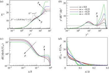
(a) Mean velocity profiles in the inner coordinates, (b) profiles of the premultiplied mean velocity derivatives in the inner coordinates, (c) profiles of the mean velocity shear in the outer coordinates and (d) mean velocity defect form normalized by
 $\unicode[STIX]{x1D6E5}=(U/u_{\unicode[STIX]{x1D70F}})\unicode[STIX]{x1D6FF}^{\ast }$
. In (a–c), the data for
 $\unicode[STIX]{x1D6FD}=0$
(
 $m=0$
),
 $\unicode[STIX]{x1D6FD}=0.73$
(
 $m=-0.15$
),
 $\unicode[STIX]{x1D6FD}=2.2$
(
 $m=-0.25$
) and
 $\unicode[STIX]{x1D6FD}=9.0$
(
 $m=-0.32$
) are extracted in the equilibrium region (
 $x/\unicode[STIX]{x1D703}_{in}=1125$
), and in (d), three streamwise locations (
 $x/\unicode[STIX]{x1D703}_{in}=1000$
, 1200, 1400) in the equilibrium region are considered for each
 $\unicode[STIX]{x1D6FD}$
to demonstrate the establishment of self-preservation. The dashed line in (b) indicates
 $1/\unicode[STIX]{x1D705}=1/0.41$
.

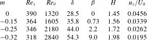
Figure 3(a) shows the mean velocity profiles normalized by the local friction velocity. All of the profiles are extracted at a fixed streamwise location in the equilibrium region (
 $x/\unicode[STIX]{x1D703}_{in}=1125$
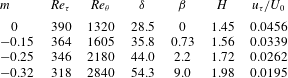
). The corresponding boundary layer parameters are shown in table 2. Consistent with previous results (Monty et al.
Reference Monty, Harun and Marusic2011; Harun et al.
Reference Harun, Monty, Mathis and Marusic2013), the velocity profiles in the log layer are shifted downward with greatly developed wake regions, and the degree of the shift becomes more significant as the APG strength increases. The velocity derivative profiles in figure 3(b) indicate that as
 $\unicode[STIX]{x1D6FD}$
increases, the slope (
 $1/\unicode[STIX]{x1D705}$
) of the log region increases and the log law of the APG TBLs moves closer to the wall. However, the wall-normal extent for the overlap region appears to be nearly constant regardless of
 $\unicode[STIX]{x1D6FD}$
in the present Reynolds number range. The mean velocity shear normalized by the outer scale variables in figure 3(c) shows that as the APG strength increases, the magnitude continuously decreases below
 $y/\unicode[STIX]{x1D6FF}=0.2$
, whereas it is increased far from the wall. Although not shown here, the inner-scaled velocity gradient profiles exhibit that the thickness of the viscous sublayer is mostly constant with respect to
 $m$
, indicating that turbulent activity in the very-near-wall region is little affected by the APGs. Figure 3(d) shows the velocity defect profiles at three streamwise locations in the equilibrium region for each value of
 $m$
. Here, the velocity and length are normalized by the local friction velocity and defect thickness
 $\unicode[STIX]{x1D6E5}=\unicode[STIX]{x1D6FF}^{\ast }(2/C_{f})^{1/2}$
(Skote et al.
Reference Skote, Henkes and Henningson1998). The velocity defect profiles for the flows almost coincide, suggesting that self-preservation is achieved in the simulations, consistent with the observation of the pressure gradient parameter (figure 2
c). Contrary to experimental findings by Skåre & Krogstad (Reference Skåre and Krogstad1994), the velocity defect profiles plotted along with
 $y/\unicode[STIX]{x1D6FF}$
are not collapsed.
Boundary layer parameters in the equilibrium region (
 $x/\unicode[STIX]{x1D703}_{in}=1125$
). Here,
 $H$
is the shape factor,
 $H=\unicode[STIX]{x1D6FF}^{\ast }/\unicode[STIX]{x1D703}$
.
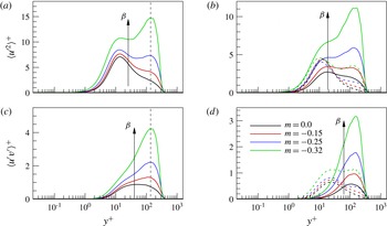
The inner-scaled streamwise Reynolds stress profiles in the equilibrium region are shown in figure 4(a). It is clear that as the pressure gradient increases, the streamwise Reynolds stresses increase throughout the boundary layer. In particular, a considerable rise of the Reynolds stress is evident in the outer layer, creating an outer peak. The outer peak locations with increasing
 $\unicode[STIX]{x1D6FD}$
are well scaled by inner scaling variables (the vertical dashed lines). When
 $m=-0.32$
(
 $\unicode[STIX]{x1D6FD}=9.0$
), the outer peak for the streamwise Reynolds stress is much larger than that of the inner peak near the wall. Harun et al. (Reference Harun, Monty, Mathis and Marusic2013) showed that when
 $\unicode[STIX]{x1D6FD}=1.74$
, there occurs a weaker secondary peak in the outer layer than that near the wall, and Monty et al. (Reference Monty, Harun and Marusic2011) reported that as
 $\unicode[STIX]{x1D6FD}$
approaches 4.74, the magnitude of the outer peak becomes similar to the near-wall peak value. The decomposition of the quantities into large- and small-scale components based on a cutoff wavelength of
 $\unicode[STIX]{x1D706}_{z}/\unicode[STIX]{x1D6FF}=0.5$
in figure 4(b) shows that the increase in the streamwise Reynolds stress in the APG flows is mostly attributed to an enhancement of the large-scale energy through the wall layer, consistent with a previous observation by Monty et al. (Reference Monty, Harun and Marusic2011). A significant increase of the large-scale energy is also shown in the Reynolds shear stress profiles in figure 4(d) with an increase in
 $\unicode[STIX]{x1D6FD}$
, although the contribution of the increased small-scale energy to the total Reynolds shear stress becomes more important near the wall relative to that of the streamwise Reynolds stress. The increased small-scale energy in the outer layer for the streamwise Reynolds stresses and Reynolds shear stresses is most likely due to the increased mean velocity shear shown in figure 3. Although not shown here, the outer-scaled Reynolds stress profiles demonstrate that the increase in the large-scale energy in the outer layer (
 $y/\unicode[STIX]{x1D6FF}>0.1$
) originates directly from the APGs.
(a) Streamwise Reynolds stress profiles with an increase in
 $\unicode[STIX]{x1D6FD}$
in the equilibrium region (
 $x/\unicode[STIX]{x1D703}_{in}=1125$
) and (b) decomposition into large- (solid lines) and small-scale (dashed lines) components. (c) Reynolds shear stress profiles with an increase in
 $\unicode[STIX]{x1D6FD}$
in the equilibrium region (
 $x/\unicode[STIX]{x1D703}_{in}=1125$
) and (d) decomposition into large- (solid lines) and small-scale (dashed lines) components. In (a,c), vertical dashed lines are shown to represent the outer peak locations.

Based on the quadrant decomposition technique with a hyperbolic hole size
 $H$
(Lu & Willmarth Reference Lu and Willmarth1973; Wallace Reference Wallace2016), the contribution of the second-quadrant ejection and fourth-quadrant sweep events to the total Reynolds shear stress can be estimated. Here, we consider two particular threshold levels,
 $H=0$
and 4, defined by
 $H=|u^{\prime }v^{\prime }|/\langle -u^{\prime }v^{\prime }\rangle$
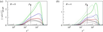
, to identify each contribution of the strong Q2 and Q4 events as the APG strength increases. Figure 5(a) shows the contributions to the conditionally averaged Reynolds shear stresses for
 $H=0$
. The solid and dashed lines indicate the contributions by Q2 and Q4 events, and the line colour legend is identical to that in figure 4. Because
 $H=0$
contains all events in each quadrant, a large number of weak events mainly contribute to the profiles. Similarly to earlier results in a turbulent channel flow (Kim, Moin & Moser Reference Kim, Moin and Moser1987), the sweep and ejection events for the ZPG TBL flow (
 $m=0$
) are dominant in the wall region (
 $y^{+}<12$
) and away from the wall (
 $y^{+}>12$
) respectively. However, as
 $\unicode[STIX]{x1D6FD}$
increases to 2.2, it is clear that the Q4-event motions become more important at approximately
 $y^{+}=100$
(blue dashed line), and a further increase in the pressure gradient reveals the dominance of the Q4 events in the range of
 $y^{+}<100$
(green dashed line). The profiles in figure 5(b) with
 $H=4$
indicate that the increase in the fourth-quadrant Reynolds shear stress in the outer layer with an increase in
 $\unicode[STIX]{x1D6FD}$
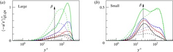
is due to large contribution of strong Q4-event motions. In addition, the decomposition of the second- and fourth-quadrant Reynolds shear stress profiles with
 $H=4$
into large- and small-scale components shown in figure 6 demonstrates that the presence of the strong Q4 Reynolds shear stress is mainly due to the large-scale components throughout the wall layer in the APG TBL flows. On the other hand, for the small-scale components in figure 6(b), the strong Q2 Reynolds shear stress is dominant in the buffer and log layers compared with those of the Q4 Reynolds shear stress.
Second- and fourth-quadrant Reynolds shear stress profiles normalized by the local friction velocity at
 $x/\unicode[STIX]{x1D703}_{in}=1125$
: (a)
 $H=0$
and (b)
 $H=4$
. In each panel, the solid and dashed lines indicate Q2- and Q4-event components, and the line colour legend is the same as in figure 4.


3.2 Turbulent structures
3.2.1 Streamwise velocity-fluctuating structures
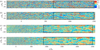
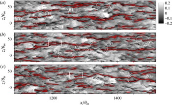
In this section, we examine the modification of large-scale structures in the log layer as the APG strength increases to identify the relationship between the APG and the large-scale features and its connection to the statistics discussed above. First, in order to gain some idea about spatial features of large-scale structures in APG flows, we visualize instantaneous streamwise velocity-fluctuating (
 $u^{\prime }$
) structures at
 $y/\unicode[STIX]{x1D6FF}=0.15$
(a nominal upper extent of the log layer). Figure 7(a,b) shows the instantaneous flow fields for ZPG and mild APG flows for the entire domain (
 $x/\unicode[STIX]{x1D703}_{in}<1500$
). In addition, figure 7(c,d) exhibits instantaneous snapshots of moderate and strong APG flows (
 $m=-0.25$
and
 $-0.32$
). It should be noted that the computational domain for the two strong APG cases with
 $m=-0.25$
and
 $-0.32$
is larger than those of the ZPG and mild APG cases due to the large growth rate of the boundary layer thickness. As shown, characteristics of outer-region large-scale turbulent structures are highly sensitive to the strength of the APG, and the development and dynamics of the structures wholly differ.
Instantaneous view of
 $u^{\prime }$
-structures normalized by
 $U_{0}$
at
 $y/\unicode[STIX]{x1D6FF}=0.15$
for ZPG and APG TBL flows. The boundary layer thickness in each panel is obtained at the centre of the computational domain. (a) Zero pressure gradient flow with
 $m=0.0$
, (b) APG flow with
 $m=-0.15$
, (c) APG flow with
 $m=-0.25$
and (d) APG flow with
 $m=-0.32$
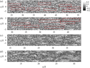
. The rectangular boxes in (a–d) are included for a detailed analysis of the flows later. The computational domain sizes for
 $m=-0.25$
and
 $-$
0.32 are larger than those for
 $m=0.0$
and
 $-$
0.15.

Because the appearance of the large-scale structures in the raw flow fields in figure 7 is very complex, with multiple scales and varying strength levels, the extraction of characteristic lines for large-scale structures is more helpful to identify the spatial organization of the structures. Here, the characteristic lines are detected based on the streak detection algorithm in Lee et al. (Reference Lee, Lee, Choi and Sung2014). The algorithm is briefly explained below.
Step 1: The instantaneous flow field is filtered using a two-dimensional Gaussian filter on the cross-stream plane to attenuate the small-scale features of
 $u^{\prime }$
. The standard deviation of the Gaussian filter along the wall-normal direction is determined based on the half-width of the two-point correlation coefficient of the streamwise velocity fluctuations with a contour of 0.5 in the spanwise direction to separate the negative
 $u^{\prime }$
-structure from adjacent negative
 $u^{\prime }$
-structures.
Step 2: Spectral low-pass filtering is applied to the Gaussian-filtered flow field with a cutoff wavelength of
 $\unicode[STIX]{x1D706}_{z}/\unicode[STIX]{x1D6FF}=0.5$
to extract the large-scale signal
 $\hat{u}$
.
Step 3: The characteristic lines (
 $CL$
s) for the large-scale structures on the
 $xz$
plane are obtained from the local extrema of the Gaussian- and low-pass-filtered field
 $\hat{u}$
:
 $$\begin{eqnarray}\displaystyle CL=\left\{\begin{array}{@{}ll@{}}1,\quad & \text{where }\unicode[STIX]{x2202}\hat{u} /\unicode[STIX]{x2202}z=0\text{ and }\hat{u} >u_{th},\\ -1,\quad & \text{where }\unicode[STIX]{x2202}\hat{u} /\unicode[STIX]{x2202}z=0\text{ and }\hat{u} <-u_{th},\\ 0,\quad & \text{otherwise}.\end{array}\right. & & \displaystyle\end{eqnarray}$$
The threshold (
 $u_{th,raw}$
) used to identify the negative
 $u^{\prime }$
-structure in the raw flow field is carefully chosen to be 10 % of the free-stream velocity (
 $U_{0}$
). In addition, because the velocity fluctuations are weakened by the two filters, the threshold value for the detection of
 $CL(u_{th})$
is corrected based on the ratio of the correlation functions, e.g.
 $u_{th}(\boldsymbol{x})=f(\boldsymbol{x})u_{th,raw}$
, where
 $f(\boldsymbol{x})=\langle u(\boldsymbol{x})\hat{u} (\boldsymbol{x}^{\prime })\rangle /\langle u(\boldsymbol{x})u(\boldsymbol{x}^{\prime })\rangle$
. For more information, the readers can refer to the earlier paper of Lee et al. (Reference Lee, Lee, Choi and Sung2014).
Instantaneous flow fields of the
 $\unicode[STIX]{x1D6FF}$
-scaled
 $u^{\prime }$
-structures in the equilibrium regions at
 $y/\unicode[STIX]{x1D6FF}=0.15$
(on the
 $xz$
plane). The boundary layer thickness in each panel is obtained at the centre of the equilibrium region. White lines indicate
 $CL=-1$
for the streamwise dimension of the negative
 $u^{\prime }$
-structures. (a) Zero pressure gradient flow, (b) APG flow,
 $m=-0.15$
, (c) APG flow,
 $m=-0.25$
, and (d) APG flow,
 $m=-0.32$
. The flow fields are extracted from the rectangular boxes in figure 7. The rectangular boxes with red dashed lines in (a,b) indicate very long structures with lengths greater than
 ${\sim}5\unicode[STIX]{x1D6FF}$
.

Figure 8 shows the instantaneous flow fields of the
 $\unicode[STIX]{x1D6FF}$
-scaled
 $u^{\prime }$
-structures in the equilibrium regions (rectangular boxes in figure 7) at
 $y/\unicode[STIX]{x1D6FF}=0.15$
. Here,
 $CL=-1$
is depicted by the white solid lines in each panel. Although the rectangular boxes for all cases are shown for the equilibrium regions in figure 7, the flows under the ZPG and APGs when
 $m=-0.15$
and
 $-0.25$
reach states of equilibrium further upstream, as shown in figure 2(c). Because the coordinate origin in the streamwise direction is defined at a location where the pressure gradient is applied in the present study, and the boundary layer thickness for each flow is obtained in the middle of the equilibrium region, the
 $x$
axis label in figure 8 differs with an increase of
 $m$
. Figure 8(a) displays that the ZPG flow includes a number of long negative
 $u^{\prime }$
-streaks (black colour contour) in the log layer with multiple scales around them with varying strengths. In particular, the rectangular boxes with red dashed lines highlight that very long meandering structures with lengths greater than
 ${\sim}5\unicode[STIX]{x1D6FF}$
travel with streamwise coherence, and the negative
 $u^{\prime }$
-structures are often inclined towards the spanwise direction at angles of approximately
 $\pm 0{-}7^{\circ }$
, consistent with earlier observations in canonical wall-bounded turbulent flows (Hutchins & Marusic Reference Hutchins and Marusic2007a
; Lee & Sung Reference Lee and Sung2011; Baltzer, Adrian & Wu Reference Baltzer, Adrian and Wu2013). As the mild APG (
 $m=-0.15$
) is applied to the TBL flow (figure 8
b), regimes of very long meandering negative
 $u^{\prime }$
-structures with lengths greater than
 ${\sim}5\unicode[STIX]{x1D6FF}$
are also found (rectangular boxes) with spanwise angles. However, as the APG strength is increased further in figure 8(c,d), the streamwise scales of structures based on the
 $CL$
s appear to be reduced in the equilibrium region, although large-scale structures are observed with large spanwise inclination angles in raw flow fields (figure 7).
The distinctive view of the large-scale
 $u^{\prime }$
-structures in figure 8 compared with the observation in the raw flow field (figure 7) for the two strong APG TBL flows is due to small-scale features in the large-scale patterns. For the ZPG TBL flow shown in figure 7(a), a long negative
 $u^{\prime }$
-structure includes multiple scales of motion with varying strengths along the streamwise direction. Several of the strong segments of the small negative
 $u^{\prime }$
-structures (the dark blue contour) appear to be streamwise-aligned coherently to create a long
 $u^{\prime }$
-structure; these small-scale motions consist of slightly streamwise-elongated negative-velocity fluctuation peaks that decay in magnitude rapidly with the distance from the peak location. A similar spatial feature of small-scale motions is observed for the mild APG flow in figure 7(b), and concatenation of the small motions induces wavering or spanwise-inclined very long motions. However, as the pressure gradient increases further, the number of strong small-scale negative fluctuations decreases significantly within the large-scale pattern, and the existing small-scale motions are scattered and disconnected but often organized along large-scale lines. Thus, the spatial organization of the
 $CL$
suggests that the small-scale structures aligned along the large-scale pattern for the strong APG flows are not coherently aligned to form large-scale structures, contrary to ZPG and mild APG flows. However, because the
 $CL$
above is identified with a relatively high threshold value, the choice of a lower threshold value captures the large-scale pattern of the
 $u^{\prime }$
-structure, similar to those in figure 7(c–d), although the identified large-scale structure is very weak in strength.
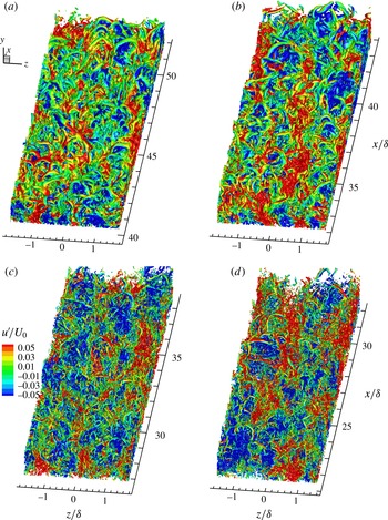
Figure 9 displays an isosurface of the swirling strength (
 $\unicode[STIX]{x1D706}_{ci}$
) from the present simulation. The data are extracted from the equilibrium region for each flow in figures 7 and 8, and the contour levels are depicted using the streamwise velocity fluctuations (
 $u^{\prime }/U_{0}$
) to identify the connection between the vortical structures and the
 $u^{\prime }$
-structures. The swirling strength
 $\unicode[STIX]{x1D706}_{ci}$
is calculated from the three-dimensional velocity gradient tensor (Zhou et al.
Reference Zhou, Adrian, Balachandar and Kendall1999). For the ZPG flow, the predominance of hairpin vortices throughout the domain is clear, with the hairpins coherently aligned in the streamwise direction to create a train of hairpins (Adrian Reference Adrian2007). Because the hairpin heads and legs induce retarded streamwise momentum beneath them, and given that the fluid in the outside of the hairpins convects downstream more rapidly due to the forward induction of the hairpins, large-scale positive and negative
 $u^{\prime }$
-structures are created. The mild APG flow in figure 9(b) also reveals a multitude of vortices and arches coherently aligned in the streamwise direction; these vortices are closely associated with the negative
 $u^{\prime }$
-structures. However, as the APG strength is increased further, it is difficult to describe the structures as an ordered hairpin forest. Most of them are significantly distorted and are oriented randomly, although individual hairpins with complete shapes are observed. Therefore, for strong APG flows, the streamwise coherence of the vortices appears to be lost, at least compared with ZPG and mild APG flows, and less streamwise coherence of the hairpins for packet organization is created. The observation in figure 9 is consistent with the spatial organization of the
 $CL$
in figure 8. Finally, it is worth mentioning that although the present observation provides clear evidence for the predominance of hairpin vortices in the ZPG and mild APG TBL flows, similar to previous studies in ZPG TBL flows up to
 $Re_{\unicode[STIX]{x1D703}}=4700$
(Adrian Reference Adrian2007; Wu & Moin Reference Wu and Moin2010; Dennis & Nickels Reference Dennis and Nickels2011a
; Jodai & Elsinga Reference Jodai and Elsinga2016), there still remain issues for the presence of a ‘forest of hairpins’ in high-Reynolds-number ZPG flow (Jiménez et al.
Reference Jiménez, Hoyas, Simens and Mizuno2010; Schlatter & Őrlü Reference Schlatter and Őrlü2012).
Isosurfaces for the swirling strength (
 $\unicode[STIX]{x1D706}_{ci}$
) in ZPG and APG flows: (a) ZPG flow, (b) APG flow,
 $m=-0.15$
, (c) APG flow,
 $m=-0.25$
, and (d) APG flow,
 $m=-0.32$
. The contour level is
 $\unicode[STIX]{x1D706}_{ci}\unicode[STIX]{x1D703}_{in}/U_{0}=0.2$
, as coloured by the streamwise velocity fluctuations (
 $u^{\prime }/U_{0}$
).

To provide statistical evidence for variation of the streamwise scales as the pressure gradient increases, two-point spatial correlations of the streamwise velocity fluctuations in the log layer are calculated for the ZPG and APG flows. The two-point correlation coefficient is defined as follows:
 $R_{uu}(r_{x},r_{y},r_{z})=\langle u^{\prime }(x_{r},y_{r},z_{r})u^{\prime }(x_{r}+r_{x},y_{r}+r_{y},z_{r}+r_{z})\rangle /\unicode[STIX]{x1D70E}_{u^{\prime }}^{2}$
, where spatial shifts from the references
 $x_{r}$
,
 $y_{r}$
and
 $z_{r}$
are represented as
 $r_{x}$
,
 $r_{y}$
and
 $r_{z}$
, with
 $\unicode[STIX]{x1D70E}_{u^{\prime }}$
as the root mean square of
 $u^{\prime }$
. For a horizontal plane,
 $r_{y}=0$
, and the correlation coefficient is independent of the reference position of
 $z_{r}$
due to flow homogeneity in the spanwise direction. In addition, although the correlation contours are shown at a fixed
 $x_{r}$
in the present study, the streamwise variation of the contours is negligible within the equilibrium region. In order to highlight large-scale features, the correlations are outer-scaled and are depicted while focusing on low contour levels (Hutchins & Marusic Reference Hutchins and Marusic2007a
; Baltzer et al.
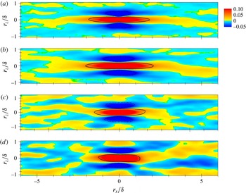
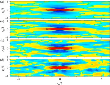
Reference Baltzer, Adrian and Wu2013). For the ZPG TBL data in figure 10(a), the general appearance of the correlation with a streamwise-elongated positive-correlation region flanked by a negative-correlation region in the spanwise direction and an X-pattern with a zero-crossing point at approximately
 $x/\unicode[STIX]{x1D6FF}=3.0{-}3.5$
is very similar to that observed in a previous experimental study of ZPG TBLs (Hutchins & Marusic Reference Hutchins and Marusic2007a
). It is noted that a spanwise symmetric condition, implying reflectional symmetry of
 $R_{uu}$
with respect to the
 $r_{z}/\unicode[STIX]{x1D6FF}=0$
line, is not applied in the calculation to show the dominant imprint of the patterns for large-scale
 $u^{\prime }$
-structures with spanwise-inclined characteristics.
Contours of two-point spatial correlations of the streamwise velocity fluctuations at
 $y_{r}/\unicode[STIX]{x1D6FF}=0.15$
. The reference streamwise location is
 $x_{r}/\unicode[STIX]{x1D703}_{in}=1125$
for each flow. (a) Zero pressure gradient flow, (b) APG flow,
 $m=-0.15$
, (c) APG flow,
 $m=-0.25$
, and (d) APG flow,
 $m=-0.32$
. The solid and dashed lines correspondingly indicate
 $R_{uu}=0.05$
and
 $-$
0.05.

Compared with the ZPG data, the APG data when
 $m=-0.15$
, as shown in figure 10(b), indicate that the streamwise scale of the large-scale structures (solid line) based on the streamwise extent of a region for which
 $R_{uu}\geqslant 0.05$
is increased with a shallow spanwise-angled X-shaped pattern (shown in yellow). However, further increase of the APG strength, shown in figure 10(c,d), causes continuous shortening of the streamwise length scales for the large-scale structures in the log layer. The X-shaped correlation patterns with large inclination angles towards the spanwise direction (shown in yellow) when
 $m=-0.25$
and
 $-$
0.32 are created by the highly spanwise-inclined structures, as observed in the instantaneous flow fields in figure 7, because the patterns of the low-level contours for the correlations can be understood as an imprint of the large- and very-large-scale structures in the flows. It should be noted that because the two-point correlations above provide averaged structures with a wide range of scales passing through the streamwise event location, small-scale structures may affect the characteristics of the large-scale structures near the event location. However, additional calculations for two-point spatial correlations of spectral-filtered large-scale streamwise velocity fluctuations with a cutoff wavelength of
 $\unicode[STIX]{x1D706}_{z}/\unicode[STIX]{x1D6FF}=0.5$
demonstrate that there is a negligible influence of the small-scale motions on our results (not shown here). As the magnitude of the APG is increased, the spanwise length scale is continuously increased in figure 10.
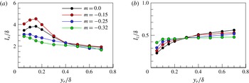
Variations of the (a) streamwise and (b) spanwise length scales based on two-point spatial correlations
 $R_{uu}$
as
 $m$
varies. The reference location in the streamwise direction is in the middle of the equilibrium region for each flow, and the length scales are extracted based on the region of
 $R_{uu}\geqslant 0.05$
, as shown in figure 9 (black solid line).

In addition to the length scales in the log layer, variations of the streamwise and spanwise length scales for several wall-normal locations from the wall are estimated in figure 11 based on
 $R_{uu}$
. For the ZPG flow, the streamwise length scale normalized by the boundary layer thickness increases to
 $y/\unicode[STIX]{x1D6FF}=0.15$
and then gradually decreases far from the wall (Lee & Sung Reference Lee and Sung2011). For the mild APG flow, although the decreasing trend is similar to that of the ZPG flow, the streamwise coherence when
 $y/\unicode[STIX]{x1D6FF}<0.4$
is larger than that for the ZPG flow. Further increase in the pressure gradient demonstrates that the streamwise length scales of the structures are continuously reduced when
 $y/\unicode[STIX]{x1D6FF}<0.4$
. However, far from the wall, the streamwise length scales for the large-scale structures are similar irrespective of the APG strength. For the spanwise length scales shown in figure 11(b), the continuous increase is obvious for
 $y/\unicode[STIX]{x1D6FF}<0.3$
as the pressure gradient increases, consistent with the observation in the instantaneous view. However, this situation is reversed far from the wall. The wall-normal variation of the length scales in figure 11 provides evidence that the streamwise coherence of the large-scale motions in the outer layer (
 $y/\unicode[STIX]{x1D6FF}<0.4$
) is not directly correlated with the energy levels of the large-scale structures in the TBLs under the APGs (figure 4). As conjectured in the introduction, the present results suggest that for a mild APG flow with an approximate range of
 $\unicode[STIX]{x1D6FD}<2.0$
, the large-scale organization pattern of the velocity fluctuations in the log layer is more elongated in the streamwise direction than that of a ZPG flow, but for moderate and strong APG flows with an approximate range of
 $\unicode[STIX]{x1D6FD}>2.0$
, the spatial coherence of the large-scale motions is shortened in the streamwise direction.
Because the log region large-scale structures for the strong APG flows are highly meandering in the spanwise direction or are spanwise-inclined due to the streamwise alignment of highly spanwise-offset streaks (Hutchins & Marusic Reference Hutchins and Marusic2007a
; Baltzer et al.
Reference Baltzer, Adrian and Wu2013), the spatial organization may mask the true streamwise length scales of
 $u^{\prime }$
-structures when measured along the
 $r_{z}=0$
line of correlations (Hutchins & Marusic Reference Hutchins and Marusic2007a
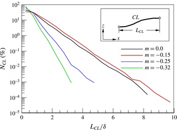
). In order to provide further evidence of the reduced streamwise coherence of strong APG flows, the ensemble-averaged population of the streamwise length scales for the lines of
 $CL=-1$
is examined. Figure 11 displays the averaged population for the streamwise length of the negative
 $u^{\prime }$
-structures (
 $L_{CL}$
) in the log layer. The population is calculated from the ratio of the number of
 $CL$
s in each length (
 $N_{CL}$
) to the total number of
 $CL$
. Although not shown, the population distribution, defined as the number of
 $CL$
s per unit area, shows a trend similar to that in the present results. It is clear that the population is highest for small-scale structures in ZPG and APG flows. For the mild APG flow with
 $m=-0.15$
, the number of large- and very-large-scale structures is slightly increased compared with the ZPG flow. The maximum streamwise length found for the mild APG flow is approximately
 ${\sim}10\unicode[STIX]{x1D6FF}$
, whereas the streamwise extent of the longest structure for the ZPG flow is approximately
 ${\sim}8\unicode[STIX]{x1D6FF}$
. As the pressure gradient is further increased, the population of the large-scale structures clearly decreases with reduced streamwise extents of the longest structures. For the strong APG flows with
 $m=-0.25$
and
 $-$
0.32, the number of small-scale structures (
 ${<}0.5\unicode[STIX]{x1D6FF}$
) accounts for more than 60 % of all negative
 $u^{\prime }$
-structures. This result indicates that the reduced streamwise coherence for the strong APG flows is mostly due to the increased population of the small-scale structures and the reduced population of the large-scale structures. It is important to note that although the population distribution for
 $u^{\prime }$
-structures is influenced by the threshold value chosen, a careful inspection of the population while varying the threshold value shows a consistent result for ZPG and APG flows due to the relatively weak streamwise coherence for strong APG flows (figure 8). Dennis & Nickels (Reference Dennis and Nickels2011b
) noted that changing the level within a reasonable margin does not alter the distribution greatly, although their algorithm differs from that in the present study. In addition, when the population distribution of the negative
 $u^{\prime }$
-structures is estimated using raw data with a threshold value (Ganapathisubramani, Longmire & Marusic Reference Ganapathisubramani, Longmire and Marusic2003; Lee & Sung Reference Lee and Sung2011; Baltzer et al.
Reference Baltzer, Adrian and Wu2013), it is confirmed that the population of large-scale structures decreases for strong APG TBL flows.
Population distribution for the streamwise length of the lines of
 $CL=-1$
in the log layer as
 $m$
is varied. The streamwise length
 $L_{CL}$
is determined by the most upstream and downstream positions of each
 $CL$
, as shown in the inset.

Identical to figure 10, but for skin-friction velocity-fluctuating structures. The solid and dashed lines indicate contour levels of 0.05 and
 $-$
0.02 respectively.

3.2.2 Skin-friction velocity-fluctuating structures
Another indication of the reduction of the streamwise coherence for the log region large-scale structures can be found based on the skin-friction features, as large-scale structures convecting in the log layer of the TBL have a clear footprint in the near-wall region (Abe, Kawamura & Choi Reference Abe, Kawamura and Choi2004; Hutchins & Marusic Reference Hutchins and Marusic2007a
; Mathis, Hutchins & Marusic Reference Mathis, Hutchins and Marusic2009; Hutchins et al.
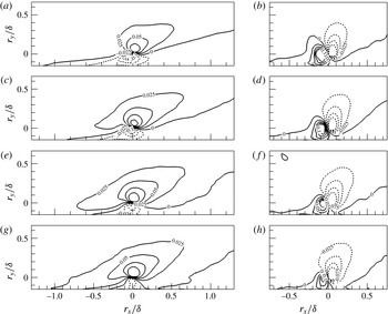
Reference Hutchins, Monty, Ganapathisubramani, Ng and Marusic2011). Figure 13 shows the two-point correlation contours for the skin-friction velocity fluctuations as the APG strength increases. As expected, the streamwise length scale for the mild APG TBL flow is longer than that for the ZPG TBL flow, consistent with the observation in figure 10. As the pressure gradient becomes stronger, the length scale is continuously shortened with larger spanwise length scales. Interestingly, the correlation in the strong APG TBL flows in figure 13(d) shows that the contours at
 $r_{x}/\unicode[STIX]{x1D6FF}=0$
are rounded, and a slight change of the contour level for large-scale structures (e.g.
 $R_{uu}=0.01$
) induces relatively large variation in the spanwise length scale, while the contours for the large-scale components in the ZPG and relatively weak APG flows in figure 13(a–c) are streamwise-elongated with little influence on the spanwise extent according to the contour level. It is noted that for the correlation of the streamwise velocity fluctuations in figure 10(d), there is no rounded contour pattern near the event location, and the choice of a contour level lower than
 $R_{uu}=0.05$
does not result in large variation in the spanwise scale of the structures. The emergence of the circular contour pattern in the correlation of the skin-friction velocity fluctuations is most likely due to the high spanwise growth rate of near-wall large-scale structures in the APG flow. Figure 11 shows that the largest increase of the spanwise length scale associated with the large-scale motions under the strongest APG flow is observed near the wall compared with the ZPG flow, while the near-wall streamwise length scale is shortened the most. The decomposition of the two-point correlation contour in figure 13(d) into large- and small-scale components shows that the rounded contour is present in the large-scale component (not shown here), supporting our conjecture.
It is reported that large-scale
 $u^{\prime }$
-structures in the log layer are closely associated with the wall-shear stress fluctuations in a turbulent channel flow (Abe et al.
Reference Abe, Kawamura and Choi2004). In addition, in a numerical study of a turbulent channel flow, Hwang (Reference Hwang2013) showed that large-scale structures with a spanwise length scale wider than
 $\unicode[STIX]{x1D706}_{z}^{+}=100$
play an important role in the generation of turbulent skin friction based on filtered simulations. For an APG flow, it is shown that the skin-friction coefficient decreases with an increase in the APG effect, as depicted in figure 2 (Lee & Sung Reference Lee and Sung2009; Monty et al.
Reference Monty, Harun and Marusic2011), and this has often been explained by the fact that the near-wall streaks are significantly weakened for the APG flow due to the wider spanwise spacing of streamwise vortices (Na & Moin Reference Na and Moin1998; Lee & Sung Reference Lee and Sung2009). In addition, in a DNS study of a turbulent channel flow with a lower curved wall, Marquillie, Ehrenstein & Laval (Reference Marquillie, Ehrenstein and Laval2011) reported that the shape and intensity of the streaks in APG wall turbulence contribute to local onset of the instability, thus modifying the self-sustained near-wall cycle mechanism (Jiménez & Pinelli Reference Jiménez and Pinelli1999). In the present study, we find that the relatively reduced streamwise coherence of the large-scale
 $u^{\prime }$
-structures in the log layer induces the shortening of the large-scale skin-friction structures responsible for the generation of the turbulent skin-friction drag in figure 13. Thus, the less coherent large-scale organization of the structures in the log layer may be another cause of the decrease in the skin-friction drag for the strong APG flows. However, the reduction of the skin-friction coefficient for the mild APG flow (
 $m=-0.15$
), while the streamwise coherence of the outer-region large-scale structures is slightly increased compared with the ZPG flow, suggests that the near-wall streamwise vortices are still important with regard to the skin-friction drag.
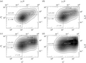
Premultiplied spanwise energy spectra of the streamwise velocity fluctuations
 $k_{z}\unicode[STIX]{x1D6F7}_{uu}/u_{\unicode[STIX]{x1D70F}}^{2}$
at
 $x_{r}/\unicode[STIX]{x1D703}_{in}=1125$
: (a) ZPG flow, (b) APG flow,
 $m=-0.15$
, (c) APG flow,
 $m=-0.25$
, and (d) APG flow,
 $m=-0.32$
. The contour level is varied from 0.2 to 2.6 in intervals of 0.2. The black and white dashed lines are shown to simplify the recognition of the inner and outer peak locations in the maps, and the dash–dot lines are to indicate the cutoff spanwise wavelength to separate large- and small-scale motions.

3.2.3 Spanwise energy spectra
In an attempt not only to provide an overall picture of the energy distributions in APG TBL flows but also to identify the dominant contribution of the wavelengths to the increase of the Reynolds stresses, premultiplied spanwise energy spectrum maps of the streamwise velocity fluctuations in the equilibrium regions are calculated. Given the two-point correlation function of each spanwise Fourier mode,
 $S_{uu}(x_{r},y_{r},k_{z})=\langle \hat{u} ^{\ast }(x_{r},y_{r},k_{z})\hat{u} (x_{r},y_{r},k_{z})\rangle$
, the spectrum in figure 14 is defined as
 $$\begin{eqnarray}\displaystyle \unicode[STIX]{x1D6F7}_{uu}(x_{r},y_{r},k_{z})=S_{uu}(x_{r},y_{r},k_{z})+S_{uu}(x_{r},y_{r},-k_{z})=2Re\{S_{uu}(x_{r},y_{r},k_{z})\}, & & \displaystyle\end{eqnarray}$$
where
 $\hat{u}$
is the spanwise Fourier component of
 $u^{\prime }$
corresponding to the wavenumber
 $k_{z}$
(
 $=2\unicode[STIX]{x03C0}/\unicode[STIX]{x1D706}_{z}$
), and the superscript
 $^{\ast }$
indicates the conjugate pair of
 $\hat{u}$
. In the figure, the cutoff spanwise wavelength of
 $\unicode[STIX]{x1D706}_{z}/\unicode[STIX]{x1D6FF}=0.5$
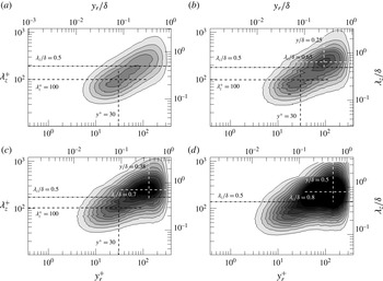
to separate large- and small-scale features is depicted by horizontal dashed dot lines. For the ZPG TBL flow in figure 14(a), an energy peak, referred to as the ‘inner peak’, is observed at
 $y^{+}=12$
with a mean spanwise wavelength of the order of 100 in wall units, i.e. a typical signature of the near-wall cycle of self-sustained quasi-streamwise vortices (Jiménez & Pinelli Reference Jiménez and Pinelli1999). Although the overall shapes of the maps are similar, the introduction of the APGs induces larger wavelength peaks with
 $\unicode[STIX]{x1D706}_{z}^{+}=120$
in the near-wall region (see the black dashed lines) for the mild and moderate APGs in figure 14(b,c). The increased wavelength of the inner peaks in the APG flows indicates that the average spanwise spacing between the streaks increases (Lee & Sung Reference Lee and Sung2009). In addition, as the APGs are applied (for
 $m=-0.15$
and 0.25), the emergence of a secondary peak in the outer layer, referred to as an ‘outer peak’, is clear, corresponding to the presence of more energetic large-scale motions in the APG flows. However, for ZPG flows, scale separation is not clear due to the low Reynolds number in the present study. As the pressure gradient increases to
 $m=-0.32$
, the strength of the outer peak increases significantly, and the peak masks the inner peak in figure 14(d) due to its strong influence on the wall. It should be noted that the rise in the outer peak with an increase in
 $\unicode[STIX]{x1D6FD}$
is not due to the scaling of the energy spectra with the friction velocity, instead originating from the APG effect. The streamwise variation of the energy spectra in figure 15 shows that the outer peak observed in the equilibrium region for
 $m=-0.32$
is created immediately when the flow moves from the ZPG to the APG. As the flow moves along the downstream direction, the strength of the outer peak increases continuously, whereas the inner peak weakens continuously due to the direct influence of the outer peak. Similarly to the outer peak, the wavelength for the inner peak of the ZPG flow rapidly shifts to a larger wavelength for an APG flow, indicating that structural modifications occur simultaneously in both the inner and outer layers.
Premultiplied spanwise energy spectra of the streamwise velocity fluctuations
 $k_{z}\unicode[STIX]{x1D6F7}_{uu}/u_{\unicode[STIX]{x1D70F}}^{2}$
for the APG flow with
 $m=-0.32$
at (a)
 $x_{r}/\unicode[STIX]{x1D703}_{in}=75$
, (b)
 $x_{r}/\unicode[STIX]{x1D703}_{in}=450$
, (c)
 $x_{r}/\unicode[STIX]{x1D703}_{in}=1125$
and (d)
 $x_{r}/\unicode[STIX]{x1D703}_{in}=2025$
. The contour level is varied from 0.2 to 2.6 in intervals of 0.2. The black and white dashed lines are shown to simplify the recognition of the inner and outer peak locations in the maps.

The presence of outer peaks in the spanwise energy spectra of the streamwise velocity fluctuations was previously reported in wall-bounded turbulent flows at a high Reynolds number (Hoyas & Jimenez Reference Hoyas and Jimenez2006; Bernardini & Pirozzoli Reference Bernardini and Pirozzoli2011). In particular, Hoyas & Jimenez (Reference Hoyas and Jimenez2006) reported that for a turbulent channel flow at
 $Re_{\unicode[STIX]{x1D70F}}=2003$
, an outer peak in the log layer with
 $\unicode[STIX]{x1D706}_{z}/\unicode[STIX]{x1D6FF}=1.4$
is aligned with an inner peak along a linear ridge, indicative of the linear growth of the spanwise length scale with the distance from the wall. Compared with previous results, however, the spectra in figure 14 reveal that the wall-normal locations of the outer peaks under the APGs (white dashed lines) are not situated at the geometrical centre of the log layer (Mathis et al.
Reference Mathis, Hutchins and Marusic2009). Moreover, the peak locations are dependent on the APG strength when normalized by the outer scale. It is noted that the outer peak locations for
 $m=-0.25$
and
 $-0.32$
are similar to those of the Reynolds stress peaks in the outer layer in figure 4, and the scaling of the outer peak locations with the inner variables is consistent with the observation of Mathis et al. (Reference Mathis, Hutchins and Marusic2009) for a ZPG TBL flow with a high Reynolds number. In figure 14, the variation of the spanwise wavelengths associated with the outer peaks with an increase in the pressure gradient indicates that as the APG becomes stronger, larger scales are more energized in the outer layer, and the emergence of horizontal contour lines for low contour levels in the outer layer suggests that the enhanced large-scale energy in the outer layer is transferred to other wavelengths. For the ZPG and mild APG flows, the low contour levels (for example, the outermost contour level, 0.2) are sloped in the maps, indicating a shift to viscous decay at a longer wavelength as the wall is approached (Wu et al.
Reference Wu, Baltzer and Adrian2012).
In figure 14(c,d), the horizontal contour lines are also found at high contour levels at approximately
 $\unicode[STIX]{x1D706}_{z}/\unicode[STIX]{x1D6FF}=0.8{-}1.0$
, suggesting that the large-scale energy in the outer layer is directly transferred to large-scale structures in the near-wall region. The stronger large-scale energy in the outer layer than that in the near-wall region for
 $m=0.32$
implies that the presence of outer peaks under APGs is not due to the linear scale growth of the small scale near the wall into the outer layer. The direct connection of the large-scale structures in the outer region and in the near-wall region in the spectra is consistent with the wall footprint of log layer large-scale structures on the inner region (Abe et al.
Reference Abe, Kawamura and Choi2004; Hutchins & Marusic Reference Hutchins and Marusic2007a
). In addition, the enhanced large-scale energy in the outer layer under APGs is consistent with a previous experimental study by Harun et al. (Reference Harun, Monty, Mathis and Marusic2013), and the large-scale energy transfer from the outer layer to the near-wall region is similar to our observation in the Reynolds stress profiles in figure 4. Although the outer peak is regarded as a symptom of the large-scale organization of the velocity field in the log layer in a ZPG TBL flow (Hutchins & Marusic Reference Hutchins and Marusic2007a
), the present findings based on the correlations and energy spectra demonstrate that the increase in the large-scale energy in the outer layer for APG TBL flows is mostly due to the presence of more energized large-scale motions in the outer layer rather than to the frequent large-scale organization of velocity fluctuations.
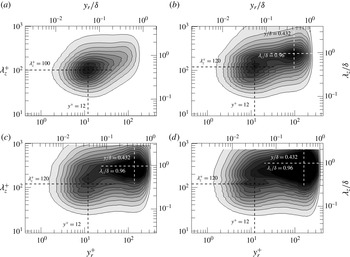
Identical to figure 14 but for premultiplied spanwise energy spectra of the Reynolds shear stress,
 $k_{z}\unicode[STIX]{x1D6F7}_{-uv}/u_{\unicode[STIX]{x1D70F}}^{2}$
. The contour level is varied from
 $-$
0.6 to
 $-$
0.05 in intervals of 0.05.

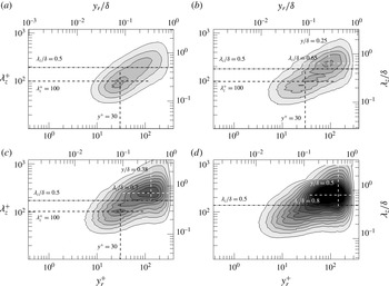
The spanwise spectrum maps for the Reynolds shear stress are presented in figure 16. Although the inner peak for the spectrum of the streamwise velocity fluctuations is dominantly characterized by approximately concentric circular contours in the ZPG flow, that in the spectrum of the Reynolds shear stress shows an inclined slope with a linear ridge between the inner and outer peaks, indicating linear spanwise growth of structures related to the Reynolds shear stress with the distance from the wall. The inner peak of the Reynolds shear stress spectra (the black dashed lines) is observed at a higher wall-normal position (
 $y^{+}=30$
) when
 $\unicode[STIX]{x1D706}_{z}^{+}=100$
compared with that for the spectra in figure 14, and the characteristics of the inner peaks are not affected by the APG strength. However, as the pressure gradient increases, the wall-normal locations for the outer peaks (the white dashed lines) move far from the wall, and larger scales of structures are more energized. Compared with the spectra of the streamwise velocity fluctuations, the outer peak locations in figure 16 are observed to be further from the wall due to the attenuation of the wall-normal velocity fluctuations near the wall, and the energy at the outer peak locations is weaker for the Reynolds shear stress spectrum map due to the less coherent structure of the Reynolds shear stress than the streamwise velocity-fluctuating structure in the outer layer.
Premultiplied spanwise energy spectra of the (a,c) second- and (b,d) fourth-quadrant Reynolds shear stresses. (a,b) Zero pressure gradient flow and (c,d) APG flow,
 $m=-0.32$
. The contour level is varied from
 $-$
0.6 to
 $-$
0.05 in intervals of 0.05.

To examine the relative contributions of the second- and fourth-quadrant Reynolds shear stresses to the spanwise energy spectra in figure 16, quadrant spectrum maps are calculated by multiplying the quadrant fractions to the energy spectra of the Reynolds shear stress,
 $$\begin{eqnarray}\displaystyle [k_{z}\unicode[STIX]{x1D6F7}_{-uv}/u_{\unicode[STIX]{x1D70F}}^{2}]_{Qi}=\frac{\langle -u^{\prime }v^{\prime }\rangle _{Qi}}{\langle -u^{\prime }v^{\prime }\rangle }k_{z}\unicode[STIX]{x1D6F7}_{-uv}/u_{\unicode[STIX]{x1D70F}}^{2},\quad i=2\text{ and }4. & & \displaystyle\end{eqnarray}$$
Figure 17 shows the spanwise energy spectrum maps for the second- and fourth-quadrant Reynolds shear stresses in the equilibrium region. For simplicity, the APG flow data for
 $m=-0.32$
are only presented in (c,d), with the ZPG flow data in (a,b). A comparison between the Q2 and Q4 spectral energy levels shows that the Q2 ejection motions play an important role in the generation of the near-wall energy peaks for both the ZPG and APG flows (a,c), although there is a slight increase in the large-scale energy of Q2 events in the outer layer under the strong APG. For the Q4-event Reynolds shear stress in figure 17(b,d), it is clear that the Q4 sweep motions contribute most to the creation of the outer peaks for the ZPG and APG flows. In particular, the large-scale Q4-event motions become increasingly important for the induction of the outer peaks, consistent with our observations in figures 5 and 6.
3.2.4 Two-point amplitude modulation
For a ZPG TBL flow, it is fairly well known that large-scale structures in the log layer modulate the amplitude of small-scale motions in the near-wall region, and as the Reynolds number increases, the amplitude modulation (AM) effect becomes progressively stronger due to the superimposition of increased large-scale activity onto the near-wall cycle (Bandyopadhyay & Hussain Reference Bandyopadhyay and Hussain1984; Mathis et al.
Reference Mathis, Hutchins and Marusic2009). For an APG TBL flow, Harun et al. (Reference Harun, Monty, Mathis and Marusic2013) estimated the degree of the AM and showed that near-wall
 $u^{\prime }$
-structures are highly modulated by the outer-region large-scale structures compared with those in a ZPG TBL flow, suggesting that the large-scale structures become more dominant in an APG flow. However, there remains the issue of which large-scale features (that is, spatial organization or energy) contribute to the enhancement of the AM effects in an APG TBL flow. In the present study, the degree of interaction between the inner and outer layers in APG TBL flows with an increase in the pressure gradient is estimated using the two-point AM covariance, which measures the modulated and modulating signals in the near-wall and outer regions simultaneously (Bernardini & Pirozzoli Reference Bernardini and Pirozzoli2011). The two-point AM coefficient is defined using the correlation between the large-scale velocity-fluctuating signal (
 $u_{L}$
) at
 $y_{1}$
and the spectral-filtered large-scale envelope of the small-scale velocity-fluctuating signal (
 $u_{EL}$
) at
 $y_{2}$
,
 $\langle u_{L}(y_{1})u_{EL}(y_{2})\rangle$
. To separate the large-scale and small-scale motions, a spanwise wavelength of
 $\unicode[STIX]{x1D706}_{z}/\unicode[STIX]{x1D6FF}=0.5$
is chosen as the cutoff wavelength (figure 14), and the envelope of the small-scale motion is extracted using the Hilbert transform.
Two-point AM covariance normalized by the local friction velocity in ZPG and APG flows: (a)
 $m=0$
, (b)
 $m=-0.15$
, (c)
 $m=-0.25$
and (d)
 $m=-0.32$
. The contour level is varied from
 $-$
0.14 to
 $-$
0.14 in intervals of 0.02, and the solid and dashed lines represent the positive and negative contour values respectively. The straight dashed lines are included to indicate the secondary outer peak locations.

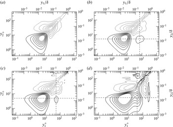
Figure 18 shows the two-point AM covariance in the equilibrium region as the APG strength increases. For the ZPG flow (figure 18
a), a clear symmetric contour is shown with respect to the diagonal line. However, an anti-symmetric contour emerges for a mild APG flow due to a secondary peak in the log layer at approximately
 $y_{1}/\unicode[STIX]{x1D6FF}=0.15$
and
 $y_{2}^{+}=5$
. As described above, this peak results from the nonlinear AM signature due to the imprints of large-scale structures in the log layer on the near-wall region. As the APG increases further, the AM effect becomes stronger and the secondary outer peak location becomes closer to the wall (
 $0.1<y/\unicode[STIX]{x1D6FF}<0.4$
). It is noted that for
 $m=-0.32$
, the modulation of the near-wall small-scale motions is induced by the large-scale structures residing over a wide range of wall-normal locations from the wall (
 $y/\unicode[STIX]{x1D6FF}<0.4$
), and thus strong contour lines in the near-wall region extend to the outer layer. The enhanced interaction between the inner and outer layers with an increase in the pressure gradient indicates that large-scale energy intensification in the outer layer is important to induce the active AM of the near-wall small-scale motions rather than the outer-region large-scale organization of streamwise velocity-fluctuating structures (figures 10 and 11). In addition, the existence of outer peaks for the AM effects in the log layer suggests that although the large-scale energy is enhanced in the vicinity of
 $0.2<y/\unicode[STIX]{x1D6FF}<0.4$
(figure 12) in the APG TBLs, the strong AM of the small-scale motions in the near-wall region is created by the log region large-scale structures, similarly to a TBL flow with a high Reynolds number (Mathis et al.
Reference Mathis, Hutchins and Marusic2009).
However, in an experimental study of APG TBL flows, Harun et al. (Reference Harun, Monty, Mathis and Marusic2013) showed that the wall-normal location of the zero-crossing for small-scale AM increases with an increase in the pressure gradient. Moreover, the wall-normal location coincides with the large-scale energetic peak location based on a one-point correlation coefficient at a wall-normal location. For the one-point correlation, a typical velocity-fluctuating signal at a wall-normal location is decomposed into large- and small-scale components, and a large-scale signal and large-scale envelope of the small-scale signal at the wall-normal location are employed to compute the correlation based on the observation that the large-scale signal at the wall-normal location is assumed to be the signature of a large-scale event in the log layer (Hutchins & Marusic Reference Hutchins and Marusic2007a
; Mathis et al.
Reference Mathis, Hutchins and Marusic2009). The two-point AM coefficient employed in the present study shows that a positive coefficient is observed up to the edge of the boundary layer, although the peak is found in the log layer. This result suggests that small-scale motions near the wall (here, at
 $y^{+}=5$
) are modulated by the large-scale motions residing throughout the boundary layer. Contrary to the present results, the presence of negative values in the one-point correlation coefficient far from the wall is due to the strong small-scale signal within the negative large-scale excursion (Harun et al.
Reference Harun, Monty, Mathis and Marusic2013).
4 Streamwise scale growth
The preceding results provide clear evidence that the streamwise length scales of the outer-region large-scale structures are significantly shortened in strong APG TBLs, although the large-scale energy in the outer layer increases continuously with an increase in the APG. In this section, we address the question of how the streamwise scales are created at different APG strengths in detail based on a conditional averaging technique and a time-evolving instantaneous flow field.
4.1 Conditional averaged flow fields
Regarding the formation of the very long
 $u^{\prime }$
-structures in the log layer, previous studies have shown that the structures in wall-bounded turbulent flows are created by the successive streamwise alignment of spatial coherence between hairpin packets (Kim & Adrian Reference Kim and Adrian1999; Lee & Sung Reference Lee and Sung2011; Baltzer et al.
Reference Baltzer, Adrian and Wu2013), although there exists an alternative explanation for the origin of the structures, which conjectures that these motions are sustained by a mechanism similar to the self-sustained process in the near-wall region (del Álamo & Jiménez Reference del Álamo and Jiménez2006). For wall-bounded turbulent flows, hairpin packets contain a number of small-scale hairpin vortices aligned along the streamwise direction and offer an explanation of the most fundamental features throughout the wall layer, such as bursting processes and quasi-streamwise vortices (Zhou et al.
Reference Zhou, Adrian, Balachandar and Kendall1999; Adrian, Meinhart & Tomkins Reference Adrian, Meinhart and Tomkins2000). In order to identify a possible cause of the modification of the large-scale features by the APGs, it is necessary to examine whether the hairpin vortices are coherently aligned to form a hairpin vortex packet in APG flows in a statistical sense.
Figure 19 shows the contours of the two-point correlations between the swirling strength and velocities in the streamwise and wall-normal directions at
 $y_{r}/\unicode[STIX]{x1D6FF}=0.15$
. Here, the swirling strength
 $\unicode[STIX]{x1D706}_{ci}$
is calculated from the two-dimensional velocity gradient tensor on the
 $xy$
plane in order to detect only spanwise swirling motion at a given location. The streamwise (
 $R_{\unicode[STIX]{x1D706}u}$
) and wall-normal (
 $R_{\unicode[STIX]{x1D706}v}$
) correlation functions for the ZPG flow are qualitatively consistent with those in Christensen & Adrian (Reference Christensen and Adrian2001) in a channel flow;
 $R_{\unicode[STIX]{x1D706}u}$
is positive above the vortex core and negative below the vortex core, and
 $R_{\unicode[STIX]{x1D706}v}$
is positive left of
 $r_{x}/\unicode[STIX]{x1D6FF}=0$
and negative right of
 $r_{x}/\unicode[STIX]{x1D6FF}=0$
. For the ZPG flow, the contours of
 $R_{\unicode[STIX]{x1D706}u}$
and
 $R_{\unicode[STIX]{x1D706}v}$
show a clear large-scale inclined interface due to the presence of hairpin heads along a line inclined away from the wall. Additionally, beneath the interface, there exists a region of relatively uniform low-momentum fluid created by the collective induction of hairpin vortices. When the APGs are applied, it is clear that the streamwise extent of the positive-
 $R_{\unicode[STIX]{x1D706}u}$
region (the high-momentum fluid) is continuously increased, while the streamwise extent of the negative-
 $R_{\unicode[STIX]{x1D706}u}$
region below the interface is significantly reduced both upstream and downstream of the reference location. As a result, the large-scale interface observed for the ZPG flow is highly suppressed, especially for the strongest APG case. For
 $R_{\unicode[STIX]{x1D706}v}$
, the negative region above the vortex core is continuously increased with an increase in the pressure gradient, and the positive region related to the negative region of
 $R_{\unicode[STIX]{x1D706}u}$
is noticeably reduced both upstream and downstream of the reference location. The increase of the negative
 $R_{\unicode[STIX]{x1D706}v}$
under the APGs indicates considerable transport of outer turbulence towards the wall for the APG cases (Skåre & Krogstad Reference Skåre and Krogstad1994), while upward transport of the near-wall turbulence is weakened.
Two-point correlations (a,c,e,g) between the swirling strength and the streamwise velocity (
 $R_{\unicode[STIX]{x1D706}u}$
) and (b,d,f,h) between the swirling strength and the wall-normal velocity (
 $R_{\unicode[STIX]{x1D706}v}$
) at
 $y_{r}/\unicode[STIX]{x1D6FF}=0.15$
: (a,b) ZPG flow, (c,d) APG flow with
 $m=-0.15$
, (e,f) APG flow with
 $m=-0.25$
and (g,h) APG flow with
 $m=-0.32$
. Contour levels are varied from
 $-$
0.1 to 0.1 with an increment of 0.025.

Linear estimates of conditional velocity fields based on a spanwise swirl at
 $y_{r}/\unicode[STIX]{x1D6FF}=0.15$
. The vectors are constructed using the conditional velocity fluctuations in figure 19. (a) Zero pressure gradient flow, (b) APG flow with
 $m=-0.15$
, (c) APG flow with
 $m=-0.25$
and (d) APG flow with
 $m=-0.32$
. The dashed lines are depicted to indicate the mean inclination angle of the structures to the wall.

In figure 20, conditional averaged velocity vector fields with a
 $\unicode[STIX]{x1D706}_{ci}$
event are shown for ZPG and APG flows to identify the vortex organization of a packet statistically. Here, the conditional averaged flow fields are approximated by LSE (Christensen & Adrian Reference Christensen and Adrian2001; Lee & Sung Reference Lee and Sung2009, Reference Lee and Sung2011; Baltzer et al.
Reference Baltzer, Adrian and Wu2013),
 $$\begin{eqnarray}\displaystyle \hat{u} _{i}(r_{x},r_{y},r_{z})=L_{i}\unicode[STIX]{x1D706}_{ci}(x_{r},y_{r},z_{r}), & & \displaystyle\end{eqnarray}$$
with
 $i=1$
, 2 and 3, and
 $$\begin{eqnarray}\displaystyle L_{i}=\frac{\langle \unicode[STIX]{x1D706}_{ci}(x_{r},y_{r},z_{r})u_{i}^{\prime }(x_{r}+r_{x},y_{r}+r_{y},z_{r}+r_{z})\rangle }{\langle \unicode[STIX]{x1D706}_{ci}(x_{r},y_{r},z_{r})^{2}\rangle }. & & \displaystyle\end{eqnarray}$$
In (4.1) and (4.2), the estimate of the conditional average is only a function of unconditional two-point correlation. In addition, because the event of the conditional average is simply a single scalar value, the character of the estimate for the conditionally averaged flow field remains the same for all values of positive
 $\unicode[STIX]{x1D706}_{ci}$
, and the magnitudes of the velocity vectors within a given estimate are amplified or attenuated depending on the chosen value of
 $\unicode[STIX]{x1D706}_{ci}$
. In the present study,
 $\unicode[STIX]{x1D706}_{ci}$
is given by the root mean square of
 $\unicode[STIX]{x1D706}_{ci}$
(
 $=\unicode[STIX]{x1D70E}_{\unicode[STIX]{x1D706}_{xi}}$
) at the reference wall-normal location (
 $y_{r}$
). The velocity vector in figure 20 is set to the unit vector to represent the relatively weak motion away from the event location more clearly. For the ZPG flow in figure 20(a), it is clear that upward motion of a low-speed fluid is observed below an inclined interface of a shear layer (
 ${\sim}13^{\circ }$
), while downward motion of a high-speed fluid is found above the interface. The large-scale inclined interface is induced by a group of spanwise-oriented vortices (Adrian et al.
Reference Adrian, Meinhart and Tomkins2000), and these vortices correspond to the heads of the hairpin-type vortices that make up a hairpin packet in the log layer. Because the flow induced from each vortex combines coherently with the flows from succeeding vortices in a packet, a region of low momentum that is significantly longer than the low-momentum region induced by any single hairpin vortex is created. The coherent alignment of the hairpin vortices in the flow direction with streamwise separation for the ZPG TBL flow is consistent with the conclusions of Zhou et al. (Reference Zhou, Adrian, Balachandar and Kendall1999) and Christensen & Adrian (Reference Christensen and Adrian2001) in turbulent channel flows and of Lee & Sung (Reference Lee and Sung2009, Reference Lee and Sung2011) in ZPG TBL flows.
For the mild APG flow, a large-scale inclined interface is also observed along the streamwise direction due to the successive alignment of the hairpins. However, around the vortex core at the event location, it is clear that the downward motion of a high-speed fluid (Q4) becomes stronger than the ZPG flow (see figure 19), and the Q2-event motions are relatively suppressed, leading to an increased inclination angle of the hairpin at the event location. As a result, the spanwise vortex core at the upstream location becomes closer to the vortex core at the event location, and the streamwise spacing between the hairpins becomes smaller than that for the ZPG flow. The increase of the Q4-event motions is consistent with the results shown in figures 5 and 6. In addition, Krogstad & Skåre (Reference Krogstad and Skåre1995) reported that turbulent motions directed towards the wall (Q4 events) last much longer near the wall for an APG flow than for a ZPG flow, whereas the frequency of Q2 events near the wall is significantly reduced. Although Lee & Sung (Reference Lee and Sung2009) showed that the streamwise length scale for a packet is increased for
 $m=-0.2$
due to the increased streamwise vortex spacing of the hairpins in the packet, the conditional averaged flow fields in figure 20(b) clearly indicate that the streamwise spacing between the hairpins is decreased when
 $m=-0.15$
due to the relatively strong Q4-event motions between the hairpins with a highly inclined shear layer angle.
As the strength of the APG increases further in figure 20(c,d), the Q4-event motions are continuously enhanced with larger inclination angles of the vortices (also see
 $R_{\unicode[STIX]{x1D706}u}$
and
 $R_{\unicode[STIX]{x1D706}u}$
in figure 19), while the Q2-event motions are significantly weakened near the event location due to the suppressed hairpins. In addition, it is clear that behind the vortex core at the event location, streamwise coherence between the spanwise-oriented vortical structures is greatly inhibited by strong high-speed fluid sweep motions compared with those in figure 20(a,b). Thus, hairpin vortices within strong APG flows do not form a vortex organization pattern for a hairpin packet coherently in the log layer, and the backward-induced flows from hairpins do not combine to produce large-scale low-speed fluid in the streamwise direction. It is noted that the dominant Q2-event motions in the log layer under strong APG flows were on small scales, as shown in figure 6. That the hairpin vortices in a flow do not form a packet suggests that large-scale motions are not concatenated to create very-large-scale motion in TBL flows subjected to strong APG, contrary to previous observations of the formation of very-large-scale motions in canonical wall-bounded turbulent flows (Kim & Adrian Reference Kim and Adrian1999; Lee & Sung Reference Lee and Sung2011; Baltzer et al.
Reference Baltzer, Adrian and Wu2013; Lee et al.
Reference Lee, Lee, Choi and Sung2014). The present observation is consistent with previous findings in the instantaneous visualization of the vortical structures shown in figure 9.
Linear estimates of large-scale conditional structures based on Q2-event vectors at
 $y_{r}/\unicode[STIX]{x1D6FF}=0.15$
. The contours are the conditional averaged streamwise velocity fluctuations normalized by the local friction velocity, and the vectors are constructed using the conditional averaged wall-normal and spanwise velocity components. (a) Zero pressure gradient flow, (b) APG flow with
 $m=-0.15$
, (c) APG flow with
 $m=-0.25$
and (d) APG flow with
 $m=-0.32$
. The streamwise vortex cores are depicted by black circles, and the solid lines indicate a contour level of
 $-$
0.3.

In order to identify the relationship between Q2-event motions and large-scale features in the log layer in a mean sense, LSE conditioned by large-scale Q2 events for ZPG and APG flows is performed on the
 $yz$
planes (figure 21). Here, the two-point spatial correlations for the LSE are obtained using spectral-filtered large-scale streamwise velocity fluctuations with a spanwise wavelength of
 $\unicode[STIX]{x1D706}_{z}/\unicode[STIX]{x1D6FF}=0.5$
to remove small-scale signatures from the flow. The Q2 event is chosen to maximize the weighted joint probability density function of large-scale streamwise and wall-normal fluctuations (Adrian Reference Adrian and Bonnet1996), and therefore makes the largest contribution to the large-scale second-quadrant Reynolds shear stress. The conditional velocity vectors in figure 21 reveal that large-scale Q2-event motions are associated with large-scale counter-rotating roll modes with centred low-speed regions for all cases, as observed in previous studies of wall-bounded turbulent flows (Toh & Itano Reference Toh and Itano2005; del Álamo & Jiménez Reference del Álamo and Jiménez2006; Hutchins & Marusic Reference Hutchins and Marusic2007b
; Chung & McKeon Reference Chung and McKeon2010; Baltzer et al.
Reference Baltzer, Adrian and Wu2013). The centred low-speed regions are flanked by high-speed events in the spanwise direction, and they extend to the near-wall region, indicating a wall footprint of a large-scale structure onto the near-wall region, irrespective of the APG strength. As the APG strength increases, the strength of the roll modes increases, consistent with the observation in figure 6. Furthermore, it is evident that the vortex core location for the roll modes moves far from the wall with wider spanwise spacing with an increase in the pressure gradient. The rise of the counter-rotating roll modes with a considerable influence on the flow under the strong APG indicates that the roll modes in strong APG TBL flows become increasingly important in organizing the entire flow.
Linear estimates of large-scale conditional structures based on Q4-event vectors at
 $y_{r}/\unicode[STIX]{x1D6FF}=0.15$
. The contours are the conditionally averaged streamwise velocity fluctuations normalized by the local friction velocity, and the vectors are constructed using the conditional averaged wall-normal and spanwise velocity components. (a) Zero pressure gradient flow, (b) APG flow with
 $m=-0.15$
, (c) APG flow with
 $m=-0.25$
and (d) APG flow with
 $m=-0.32$
. In the panels, the streamwise vortex cores for the Q2 events are depicted by black circles for a comparison with the cores obtained from the Q4 events, and the solid lines indicate a contour level of 0.3.

Figure 22 shows linearly estimated large-scale conditional structures based on large-scale Q4 events in the log layer not only to examine the structural difference between the structures related to Q2 and Q4 events but also to identify the cause of the magnitude difference in the second- and fourth-quadrant Reynolds shear stresses in figures 5 and 6. The procedure for the calculation here is identical to that used for the large-scale Q2 event in figure 21, the only difference being the given conditions. To identify the structural differences between the large-scale Q2- and Q4-related motions quantitatively, solid contour lines are presented for contour levels of
 $-$
0.3 and 0.3 in figures 21 and 22, with black circles for the streamwise vortex cores associated with the Q2 events depicted in figures 21 and 22. Similarly to the large-scale Q2-event motions, the dominant large-scale Q4-event motions are counter-rotating large-scale roll modes in APG flows. The high-speed regions are located in the middle of the domain and are surrounded by the low-speed regions in the spanwise direction. The high-speed regions also extend to the near-wall region, and the strength increases with an increase in the pressure gradient. However, an obvious difference between the large-scale Q2- and Q4-event motions arises, in which the roll modes related to Q4 events are stronger, with a greater influence on the flow than those of Q2 events (comparing the solid lines and black circles). These strong large-scale roll modes greatly intensify the large-scale fourth-quadrant Reynolds shear stress in figure 6 compared with the effect on the second-quadrant Reynolds shear stress. Because the large-scale roll modes centred in the outer layer can sweep the near-wall smaller scales of motions in wall-bounded turbulent flows to organize along the lines of the roll modes (Toh & Itano Reference Toh and Itano2005; Baltzer et al.
Reference Baltzer, Adrian and Wu2013), the presence of the stronger roll modes can lead to more active turbulence motions beneath the roll mode pattern with large AM effects. The upward shift of the large-scale roll modes for the APG flows compared with the ZPG flow is consistent with a previous finding of Bradshaw (Reference Bradshaw1967), who observed a rise of the low-frequency energetic content in the outer region based on a spectral analysis of an APG flow.
Temporal evolution of the negative
 $u^{\prime }$
-structures (
 $u^{\prime }/U_{0}$
) at
 $y/\unicode[STIX]{x1D6FF}=0.15$
for an APG flow with
 $m=-0.15$
. The red solid lines indicate
 $CL=-1$
. The flow field in figure 23(b) is extracted from figure 7(b). The negative
 $u^{\prime }$
-structures at the reference time step
 $t_{r}$
(figure 23
b) are temporally traced with time interval
 $\unicode[STIX]{x0394}t^{+}$
: (a)
 $t_{r}-\unicode[STIX]{x0394}t^{+}$
and (b)
 $t_{r}+\unicode[STIX]{x0394}t^{+}$
, where
 $\unicode[STIX]{x0394}t^{+}=88.2$
. The merging events between negative
 $u^{\prime }$
-structures (A–D) are highlighted by ellipses with white dashed lines. The breaking event is depicted by a rectangle with a white solid line.

4.2 Time-resolved instantaneous flow fields
Although the vortex organization of a hairpin packet indicates a reduction of the streamwise coherence of the vortices in the streamwise direction statistically (figures 19 and 20), the two-point spatial correlations for the negative
 $u^{\prime }$
-structures in the log layer show evidence of an increase in the streamwise length scales for the large-scale structures in the mild APG TBL flow, compared with the ZPG TBL flow (figures 10 and 11). The population distribution of the negative
 $u^{\prime }$
-structures in figure 12 indicates that the presence of a larger population of large-scale structures for the mild APG TBL flow than that for the ZPG flow induces greater streamwise coherence of the negative
 $u^{\prime }$
-structures in the correlations. In order to provide a proper explanation for the increase of the length scale in large-scale
 $u^{\prime }$
-structures for a mild APG flow, the time-resolved instantaneous flow fields of the
 $u^{\prime }$
-structures are analysed. The main idea is that small scales organize coherently to create a large scale in the flow field, as supported by Kim & Adrian (Reference Kim and Adrian1999), Lee & Sung (Reference Lee and Sung2011), Baltzer et al. (Reference Baltzer, Adrian and Wu2013) and Lee et al. (Reference Lee, Lee, Choi and Sung2014).
Figure 23 shows the temporal evolution of the negative
 $u^{\prime }$
-structures for an APG flow (
 $m=-0.15$
) with a time interval of
 $\unicode[STIX]{x0394}t^{+}=88.2$
. The red lines indicate the position of
 $CL=-1$
. The flow field in figure 23(b) is extracted from figure 7(b) to analyse the temporal variation of the negative
 $u^{\prime }$
-structures, and figure 7(a) and (c) show the flow fields at the previous (
 $t_{r}-\unicode[STIX]{x0394}t^{+}$
) and next (
 $t_{r}+\unicode[STIX]{x0394}t^{+}$
) time steps, compared with that at the reference time step (
 $t_{r}$
) in figure 23(b). The time variance of the structures displays many merging events between multiple structures. Here, the merging event is defined when the negative
 $u^{\prime }$
-structures presented at the previous time step are merged to form a single long structure at the next time step. The ellipses with white dashed lines highlight several merging events between negative
 $u^{\prime }$
-structures. In particular, two large-scale structures (marked as ‘B’) with streamwise extents larger than
 ${\sim}3\unicode[STIX]{x1D6FF}$
at
 $t=t_{r}-\unicode[STIX]{x0394}t^{+}$
become a single long
 $u^{\prime }$
-structure at
 $t=t_{r}+\unicode[STIX]{x0394}t^{+}$
. The merging event (marked as ‘A’) corresponds to a merging event between the large- and small-scale structures. In addition to the merging event, the rectangle with a white solid line suggests that the large-scale structure at
 $t=t_{r}$
is fractured into small- and large-scale structures at
 $t=t_{r}+\unicode[STIX]{x0394}t^{+}$
, indicating a breaking event of the negative
 $u^{\prime }$
-structure. Lee et al. (Reference Lee, Lee, Choi and Sung2014) categorized the time variance characteristics of the negative
 $u^{\prime }$
-structures into the six events of preserving, merging, breaking, growing, shortening, creating and extinction, and showed that the merging event is dominant in the near-wall region and the outer layer.
Figure 24 shows a three-dimensional visualization of the negative
 $u^{\prime }$
-structures prior to a merging event to provide a general understanding of this process. The flow fields in (a,c) are identical to those in figure 23(a,b), and the merging event (marked as ‘A’) is scrutinized in detail. The dark and light grey isocontours represent the regions of
 $y/\unicode[STIX]{x1D6FF}<0.15$
and
 $y/\unicode[STIX]{x1D6FF}\geqslant 0.15$
. Consistent with the observation above, the negative
 $u^{\prime }$
-structures at
 $t=t_{r}-\unicode[STIX]{x0394}t^{+}$
are separated in the streamwise direction, and as the structures move along the downstream direction, the outer structures continuously merge due to the narrowing of the streamwise gap. The observed merging event for the mild APG TBL flow can be explained by the convection velocity difference in the upstream and downstream structures (Lee et al.
Reference Lee, Lee, Choi and Sung2014). Because the magnitude difference of
 $u^{\prime }$
leads to the convection velocity difference, the upstream head (UH: the most downstream position of an upstream
 $u^{\prime }$
-structure) of the weak negative
 $u^{\prime }$
-structure convects more rapidly than the downstream tail (DT: the most upstream position of a downstream structure) of the strong negative
 $u^{\prime }$
-structure. As a result, the two adjacent structures are merged in the streamwise direction, creating a longer
 $u^{\prime }$
-structure.
Isosurfaces of the streamwise velocity fluctuations (
 $u^{\prime }=0.1U_{0}$
) at (a)
 $t_{r}-\unicode[STIX]{x0394}t^{+}$
, (b)
 $t_{r}-1/2\unicode[STIX]{x0394}t^{+}$
and (c)
 $t_{r}$
. The flow fields in (a) and (c) are extracted from the rectangle with the white dashed line in figure 23. The dark and light grey colours indicate
 $y/\unicode[STIX]{x1D6FF}<0.15$
and
 $y/\unicode[STIX]{x1D6FF}\geqslant 0.15$
. The upstream head of a downstream structure and the downstream tail of a downstream structure are denoted by UH and DT respectively. The ellipse in (c) indicates a merging event of two negative
 $u^{\prime }$
-structures.

Time sequence of the conditionally averaged velocity fields of the streamwise velocity fluctuations (
 $u^{\prime }/U_{0}$
) on the
 $xy$
plane (
 $r_{z}/\unicode[STIX]{x1D6FF}=0$
) for a mild APG TBL flow. The condition is given by a merging event between the negative
 $u^{\prime }$
-structures at
 $t_{r}$
, for (a)
 $r_{t}^{+}=-6\unicode[STIX]{x0394}t^{+}$
, (b)
 $-4\unicode[STIX]{x0394}t^{+}$
, (c)
 $-2\unicode[STIX]{x0394}t^{+}$
and (d)
 $-\unicode[STIX]{x0394}t^{+}$
. Here,
 $\unicode[STIX]{x0394}t^{+}=11.1$
. The contour levels are varied from
 $-$
0.11 to
 $-$
0.04 with an increment of 0.002. The solid line indicates a contour of
 $-$
0.05.

Because the merging event proposed above is evaluated based on a single flow field, it cannot be generalized to explain the streamwise scale growth of the
 $u^{\prime }$
-structures for a mild APG TBL flow. In order to provide statistical evidence of the scale growth caused by merging, conditional averaging with a merging event between two negative large-scale
 $u^{\prime }$
-structures is conducted. The conditionally averaged velocity field is defined as follows (Lee et al.
Reference Lee, Lee, Choi and Sung2014):
 $$\begin{eqnarray}\displaystyle \tilde{u} (r_{x},r_{y},r_{z};r_{t})=\langle u^{\prime }(x_{r}+r_{x},y_{r}+r_{y},z_{r}+r_{z};t_{r}-r_{t})|CL^{DT}(x_{r},y_{r},z_{r};t_{r})\rangle , & & \displaystyle\end{eqnarray}$$
where (
 $x_{r},y_{r},z_{r}$
) refers to the reference location being the tail position of the downstream structure at reference time
 $t_{r}$
. The time series are obtained by conditionally averaging the velocity fields while varying
 $r_{t}$
relative to the merging instant
 $t_{r}$
. A time sequence of a conditionally averaged flow field for a mild APG flow is shown in figure 25. The solid line indicates a relatively strong negative
 $u^{\prime }$
-structure. Although the reference position (
 $x_{r}=0$
) for the conditional average is given at the tail of the downstream structure, another velocity signature for a negative
 $u^{\prime }$
-structure is shown upstream of the reference position. At
 $t_{r}-6\unicode[STIX]{x0394}t^{+}$
, the downstream structure has a ramp-shaped tail downstream of the merging event, and the head of the upstream structure arises at approximately
 $r_{x}/\unicode[STIX]{x1D6FF}=-1.0$
. The upstream structure is clearly separated from the downstream structure, with a relatively small streamwise gap distance (solid line), and the two structures are in-line. Although
 $u^{\prime }$
-structures are aligned in the streamwise direction and are spanwise-offset in the instantaneous field (figure 7), the inherent symmetry of the structures in the spanwise direction induces the in-line
 $u^{\prime }$
-structures in the conditional field. As the structures convect along the downstream direction, the two adjacent structures gradually merge to form a longer negative
 $u^{\prime }$
-structure at
 $t_{r}$
. A similar merging process between negative
 $u^{\prime }$
-structures is also observed for a ZPG TBL flow (not shown here). However, because there are many wider structures in an APG TBL flow compared with a ZPG TBL flow, as documented through the instantaneous and statistical analyses (figures 7 and 11), merging events for streamwise scale growth are expected to occur more frequently for APG TBL flows (Lee, Kim & Lee Reference Lee, Kim and Lee2016). The number of merging events per unit area for APG TBL flows is increased by approximately 10 % compared with that for ZPG TBL flows, leading to a slightly larger population of large-scale
 $u^{\prime }$
-structures for mild APG TBL flows. Interestingly, the rate of increase is very similar to the ratio of the spanwise length scales between the APG and ZPG TBL flows shown in figure 11. When used with identical procedures for conditional averaging with a merging event for strong APG TBL flows, no clear evidence of a merging event between
 $u^{\prime }$
-structures is observed due to the absence of adjacent large-scale
 $u^{\prime }$
-structures.
5 Summary and conclusions
In the present study, we performed DNS of spatially developing TBLs subjected to mild (
 $\unicode[STIX]{x1D6FD}=0.73$
), moderate (
 $\unicode[STIX]{x1D6FD}=2.2$
) and strong (
 $\unicode[STIX]{x1D6FD}=9.0$
) APGs to examine the structural modifications of large-scale features in the log layer, motivated by a literature review of APG TBL flows in which inconsistencies exist with regard to the effect of the pressure gradient on the large-scale structures in the log layer. The instantaneous flow fields and two-point spatial correlations of the streamwise velocity-fluctuating structures showed that the spatial organization of the
 $u^{\prime }$
-structures in the log layer is strongly influenced by the pressure gradient. For a mild APG flow (
 $\unicode[STIX]{x1D6FD}<2.0$
), the streamwise coherence of the
 $u^{\prime }$
-structures was increased compared with that in the ZPG TBL flow. However, as the APG increased (
 $\unicode[STIX]{x1D6FD}>2.0$
), the streamwise length scales of the
 $u^{\prime }$
-structures were clearly reduced in the log layer. Consistent variation of the streamwise length scales with respect to the pressure gradient was found below
 $y/\unicode[STIX]{x1D6FF}=0.4$
. On the other hand, the spanwise length scales continuously increased with an increase in the pressure gradient for
 $y/\unicode[STIX]{x1D6FF}<0.3$
, whereas they were decreased far from the wall. Another indication of the influence of the pressure gradient on the large-scale organization in the log layer was provided based on skin-friction features, because the log region large-scale structures have strong imprints on the near-wall region. An inspection of the two-point spatial correlations of the skin-friction velocity-fluctuating structures showed that the variation of the streamwise length scales of the structures with respect to the pressure gradient is consistent with that of the outer region large-scale
 $u^{\prime }$
-structures, which implies that the decrease in the skin-friction drag with an increase in the pressure gradient is partially due to the reduction of the streamwise coherence of the log region large-scale structures.
The analysis of the spanwise energy spectra of the streamwise velocity fluctuations in APG TBL flows revealed that the dominant inner peaks occur at
 $y^{+}=12$
with a larger spanwise wavelength of
 $\unicode[STIX]{x1D706}_{z}^{+}=120$
, indicative of the increased mean spanwise spacing of the streaks in the near-wall region. In addition, as the APG strength increased, the second dominant outer peaks emerged above the log layer, and the strength of the outer peaks was increased, consistent with the streamwise Reynolds stresses. When the APG became stronger, larger scales became more energized in the outer layer and the outer-region large-scale energy was directly linked to near-wall large-scale structures, supporting the outer-region large-scale imprint onto the near-wall region. The increase of the large-scale energy in the outer layer for APG TBL flows was mostly due to the presence of more energized large-scale motions in the outer layer than the frequent large-scale organization of the velocity field. The analysis of the two-point AM covariance showed that as the APG is increased, the AM effect becomes stronger with secondary outer peaks. The enhanced interaction between the inner and outer layers with an increase in the pressure gradient indicated that the large-scale energy intensification in the outer layer plays an important role in inducing the active near-wall small-scale AM rather than that of the outer-region large-scale velocity organization. Furthermore, the existence of outer peaks in the AM effects in the log layer suggested that although the large-scale energy is enhanced particularly above the log layer (
 $0.2<y/\unicode[STIX]{x1D6FF}<0.4$
) in APG TBLs, the AM of the near-wall small-scale motions is dominantly created by the log region large-scale energy.
In order to address the question of how the streamwise scales of
 $u^{\prime }$
-structures are influenced by the degree of the pressure gradient in the TBLs, the conditional averaged flow fields were analysed in detail. Conditional structures with a spanwise swirling event showed that the hairpin vortices are coherently aligned to form a hairpin vortex packet in the log layer for a mild APG TBL flow, similar to that in a ZPG flow. However, as the pressure gradient became stronger, the spanwise-oriented vortical structures were greatly inhibited and the hairpin vortices within the strong APG flows did not form a vortex organization pattern for a hairpin packet coherently. The absence of the statistical signature of a hairpin packet in the strong APG TBL flows indicated that large-scale motions are not concatenated to create very-large-scale motion in strong APG flows, resulting in a reduction of the streamwise coherence of the
 $u^{\prime }$
-structures in the log layer. The suppression of the hairpin vortices in the strong APG TBL flows was closely associated with large-scale counter-rotating roll modes identified with Q2- and Q4-event conditions. The conditional roll modes showed that although these roll modes become increasingly important in organizing the entire flow as the pressure gradient increases, the large-scale roll modes related to the Q4 events are much stronger with a greater influence on the flows than those related to Q2 events. Because the large-scale roll modes centred in the outer layer could collect small-scale motions to organize along the lines of the roll modes near the wall, the presence of strong roll modes in APG flows can lead to active turbulence activity for the fourth-quadrant Reynolds shear stress beneath the roll mode pattern.
Based on the time-resolved instantaneous flow fields for
 $u^{\prime }$
-structures, the increase in the streamwise length scale for the large-scale
 $u^{\prime }$
-structures in a mild APG flow, compared with ZPG TBL flow, was attributed to the more active merging event between adjacent
 $u^{\prime }$
-structures induced by the increased spanwise length scale of the structures for the APG flow. Consistent with canonical wall-bounded turbulent flows (Lee & Sung Reference Lee and Sung2011; Lee et al.
Reference Lee, Lee, Choi and Sung2014), the observed merging event for a mild APG TBL flow was explained by the convection velocity difference between the upstream and downstream structures. Because the magnitude difference of
 $u^{\prime }$
induced the convection velocity difference, the upstream head of the weak negative
 $u^{\prime }$
-structure moved more rapidly downstream than the downstream tail of the strong negative
 $u^{\prime }$
-structure. As a result, the two adjacent structures were merged in the streamwise direction, creating a longer
 $u^{\prime }$
-structure. However, as the APG strength increased further, the
 $u^{\prime }$
-structures were often separated with large streamwise gap distance due to less coherence of hairpin vortices, and the streamwise merging event for the formation of the longer structure was not observed statistically.
Acknowledgements
This research was supported by a Basic Science Research Program through the National Research Foundation of Korea (NRF) funded by the Ministry of Education (NRF-2014R1A1A2057031).