



1. Introduction and the formula for the perimeter
The isoperimetric inequality states that among all subsets of  $ \mathbb{R}^m $ with a given volume, the sphere minimizes the perimeter. More precisely:
 \begin{equation*}
P(E) \geq C_m |E|^{\frac{m-1}{m}},
\end{equation*}
where  $ P(E) $ is the perimeter,
 $ |E| $ is the volume, and
 $C_m = m \, \omega_m^{1/m},
$ where
 $\omega_m$ denotes the volume of the unit ball in
 $\mathbb{R}^m$. Equality holds if and only if
 $ E $ is a sphere.
1.1. Fuglede’s stability theorem [Reference Fuglede3]
While the classical inequality identifies spheres as optimal shapes, Fuglede’s theorem addresses the question of stability: How close is a set  $ E $ to a sphere if its perimeter nearly minimizes the isoperimetric inequality?
Fuglede’s result provides a quantitative estimate linking the deficit:
 \begin{equation*}
\delta(E) = P(E) - C_m |E|^{\frac{m-1}{m}},
\end{equation*}
to the geometric deviation of  $ E$ from a sphere. Specifically:
• If
 $ \delta(E) $ is small, then
$E $ is close (in an appropriate metric) to a spherical domain with the same volume.


The paper [Reference Fusco, Maggi and Pratelli4] by Fusco, Maggi, and Pratelli is a substantial contribution to the study of isoperimetric inequalities. It advances the understanding of how the isoperimetric deficit, defined as
 \begin{equation*}
D(E) = \frac{P(E)}{C_m |E|^{(m-1)/m}} - 1,
\end{equation*}
and the Fraenkel asymmetry,
 \begin{equation*}
\lambda(E) = \min \left\{\frac{|E \Delta (x + rB)|}{r^m} : x \in \mathbb{R}^m, \ |rB| = |E| \right\},
\end{equation*}
are related. The results are pivotal in the field and significantly refine the classical isoperimetric inequality.
1.2. Extensions to hyperbolic space
The extension of the isoperimetric inequality to hyperbolic space has been given by Schmidt in [Reference Schmidt17]. In the hyperbolic space  $ \mathbb{H}^m $, the geometry is non-Euclidean, and the isoperimetric inequality takes a different form, reflecting the curvature of the space. Here, geodesic spheres minimize the isoperimetric ratio.
V. Bögelein, F. Duzaar, and C. Scheven [Reference Bögelein, Duzaar and Scheven1] extended stability results to hyperbolic settings. They showed that:
(1) A quantitative stability result analogous to Fuglede’s holds in
$ \mathbb{H}^m $.(2) The deficit in the hyperbolic isoperimetric inequality controls the deviation of a domain from a geodesic sphere.

The Bergman ball in  $\mathbb{C}^n$ serves as a counterpart to hyperbolic space. In the case
 $n = 1$ (i.e., for the complex unit disk), these two spaces coincide, but for
 $n \gt 1$, they exhibit significant differences. A central open problem in this context is the isoperimetric inequality for subsets of the Bergman ball, which is the unit ball in complex space endowed with the Bergman metric. This question remains an intriguing challenge in complex geometry and analysis.
While isoperimetric inequalities have been extensively studied in classical hyperbolic spaces and other standard geometric settings, the Bergman ball presents unique difficulties due to the intrinsic properties of the Bergman metric, which is neither isotropic nor conformally flat, unlike the hyperbolic metric. A particularly interesting question is whether the extremal sets for such an isoperimetric inequality are Euclidean balls centred at the origin and their holomorphic images. Evidence supporting this conjecture is provided in this paper. Establishing such an inequality would lead to the determination of the isoperimetric profile of the Bergman ball (for a discussion of isoperimetric profiles, see [Reference Ritoré15]).
A recent attempt at solving this problem appears in [Reference Li and Su.7]. Moreover, proving this inequality would have implications for the Lieb–Wehrl entropy conjecture in the context of 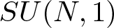 $SU(N,1)$ (see [Reference Kumar and Singh11]). In the one-dimensional case, the result was established by Kulikov in [Reference Kulikov10] using the isoperimetric inequality for the hyperbolic disk.
The stability framework unifies understanding across Euclidean and non-Euclidean geometries, emphasizing the robustness of optimal shapes under perturbations. The Faber–Krahn inequality is essentially a spectral isoperimetric inequality. It emerges from the same principle as the isoperimetric inequality: balls are optimal shapes for fundamental optimization problems in geometry and analysis. The stability of Faber–Krahn inequality for the short-time Fourier transform published in [Reference Gómez, Guerra, Ramos and Tilli6] is also based on the Euclidean isoperimetric inequality.
1.3. Bergman unit ball
Let  $\mathbb{B}_n=\{z\in\mathbb{C}^n: \vert z\vert \lt 1\}$ be the unit ball in
 $\mathbb{C}^n$. The boundary of
 $\mathbb{B}_n$ will be denoted by
 $\mathbb{S}$. Let
 $ \upsilon$ denote the Euclidean volume measure on
 $\mathbb{B}_n$. The
 $2n-1$ dimensional Hausdorff measure will be denoted by
 $\mathcal{H}$ and by
 $d\mathcal{H}$ its area element. By
 $\mathbb{B}_r$, we denote the ball
 $|z| \lt \tanh(r/2)$.
The Bergman metric in the unit complex ball  $ \mathbb{B}_n = \{z \in \mathbb{C}^n : | z | \lt 1 \} $ is defined as follows [Reference Rudin16]: Firstly, define the Bergman kernel on
 $ \mathbb{B}_n $ by
 \begin{equation*}
K(z, w) = \frac{1}{(1 - \langle z, w \rangle)^{n+1}}
\end{equation*}
where  $ \langle z, w \rangle = z_1 \overline{w_1} + z_2 \overline{w_2} + \cdots + z_n \overline{w_n} $ is the standard Hermitian inner product on
 $ \mathbb{C}^n $. The real inner product is then defined by
 $ \langle z, w \rangle_R =\Re \langle z, w \rangle$. We use the normalized Bergman metric, obtained by dividing
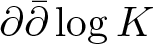 $\partial\bar\partial\log K$ by the factor
 $n+1$. Thus, the Bergman metric is defined by the matrix
 $ B(z) = \{g_{i\bar{j}}(z) \}_{i,j=1}^n $, where
 \begin{equation*}
g_{i \bar{j}}(z) = \frac{1}{n+1}\frac{\partial^2}{\partial z_i \, \partial \overline{z_j}} \log K(z, z),
\end{equation*}
which provides the components of the metric tensor in this normalization.
In the unit ball  $ \mathbb{B}_n $, this can be computed explicitly as:
 \begin{equation*}
g_{i \bar{j}}(z) = \frac{(1 - | z |^2) \delta_{ij} + \overline{z_i} z_j}{(1 - | z |^2)^2}.
\end{equation*}
Its inverse is given by the following entries,
 \begin{equation*}
g^{i \bar{j}}(z) = (1 - | z |^2) (\delta_{ij} - \overline{z_i} z_j).
\end{equation*}
1.4. The Bergman perimeter of a set in the Bergman ball
The aim of this section is to find the formula for the perimeter of a level set in the Bergman ball. The measure (fundamental form) on the Bergman ball is defined by
 \begin{equation*}d\mu(z) = (1-|z|^2)^{-n-1} d\upsilon(z),\end{equation*}
where  $d\upsilon(z)$ is the
 $2n$ dimensional Lebesgue measure. So the Bergman measure of a set
 $E\subset \mathbb{B}$ is given by
 \begin{equation*}\mu(E) = \int_{E} d\mu (z).\end{equation*}
Assume that  $U$ is a smooth real function defined in the unit ball, and assume that
 \begin{equation*}M=\{z\in\mathbb{B}: U(z)=c\}\end{equation*}
is compactly supported in  $\mathbb{B}$.
For a point 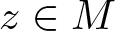 $z\in M$, let
 $N=\nabla_b U/|\nabla_b U|_b$ be the unit normal induced by the Bergman metric at
 $M$. Assume
 $\sigma_g$ is the volume form in
 $\mathbb{B}$, and let
 $\sigma_{\tilde g}$ be the induced area form in
 $M$. We use the formula
 \begin{equation}
\tilde \sigma=\sigma_{\tilde g}=\iota^\ast_M(N\lrcorner \sigma_g)\end{equation}
see [Reference Lee13, Proposition 15.32]. Now we find the unit normal vector field. We first have
 \begin{equation*} \nabla_b U= \sum_{i,j=1}^n g^{i\bar{j}}(z) \frac{\partial U}{\partial \overline{z_j}}\frac{\partial}{\partial z_i}.\end{equation*}
Then
 \begin{equation*}\nabla_b U = (1-|z|^2)((1-|z_1|^2)U_{\overline{z}_1}-\sum_{k=2}^n z_1\overline{z_k}U_{\overline{z}_k},\dots,
(1-|z_n|^2)U_{\overline{z}_n}-\sum_{k=1}^{n-1} z_n\overline{z_k}U_{\overline{z}_k}).\end{equation*}
Here,  $\nabla U$ denotes the Euclidean gradient of the real-valued function
 $U$ on
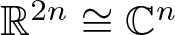 $\mathbb{R}^{2n}\cong\mathbb{C}^n$. In the following computation,
 $\nabla_b U$ is identified with the corresponding real vector field, and
 $\langle\cdot,\cdot\rangle$ denotes the real Euclidean pairing. We compute
 \begin{equation*}
\begin{aligned}
\left \lt \nabla_b U, \nabla U\right \gt &= (1-|z|^2)\left((1-|z|^2) |\nabla U|^2 + \sum_{1\le j \lt k\le n}|z_k U_{\bar{z}_j}-z_j U_{\bar z_k}|^2\right)
\\ &=(1-|z|^2)\left( (1-|z|^2) |\nabla U|^2 + |z|^2 |\nabla U|^2 - |\left \lt z,\nabla U\right \gt |^2\right)
\\ &= (1-|z|^2)(|\nabla U|^2-|\left \lt z,\nabla U\right \gt |^2).
\end{aligned}
\end{equation*}
We also have
 \begin{equation*}|\nabla_b U|_b^2 = \left \lt \nabla_b U, \nabla U\right \gt .\end{equation*}
This implies the formula
 \begin{equation}
\left \lt \frac{\nabla_b U}{|\nabla_b U|_b}, \frac{\nabla U}{|\nabla U|}\right \gt = \sqrt{1-|z|^2}\sqrt{1-\left|\left \lt \frac{\nabla U}{|\nabla U|}, z\right \gt \right|^2}.
\end{equation}
The inner product between two vectors  $V_1, V_2$ in the Bergman ball is given by
 \begin{equation*}\left \lt V_1, V_2\right \gt _b= \Re[\left \lt B(z)V_1, V_2\right \gt ].\end{equation*}
Now for  $V_1=\nabla_b U$, we have
 $B(z) V_1 = c \nabla U,$ with
 $c \gt 0$. From this, we see that
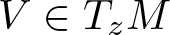 $V\in T_zM$ w.r.t. Bergman structure if and only if
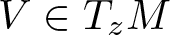 $V\in T_zM$ w.r.t. Euclidean structure of
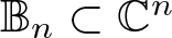 $\mathbb{B}_n\subset \mathbb{C}^n$.
Then from (1.1) and (1.2), for vectors  $v_1,\dots, v_{2n-1}$ from
 $T_zM$, we find that
 \begin{equation*}\begin{aligned} \tilde \sigma(v_1, \dots, v_{2n-1})&=\mu\left(\frac{\nabla_b U}{|\nabla_b U|_b}, v_1, \dots, v_{2n-1}\right)
\\[3pt] & =(1-|z|^2)^{-n-1}\upsilon\left(\frac{\nabla_b U}{|\nabla_b U|_b}, v_1, \dots, v_{2n-1}\right)
\\[3pt] &= (1-|z|^2)^{-n-1}\left \lt \frac{\nabla_b U}{|\nabla_b U|_b}, \frac{\nabla U}{|\nabla U|}\right \gt \upsilon\left(\frac{\nabla U}{|\nabla U|},v_1, \dots, v_{2n-1}\right)
\\[3pt] &=(1-|z|^2)^{-n-1} \left \lt \frac{\nabla_b U}{|\nabla_b U|_b}, \frac{\nabla U}{|\nabla U|}\right \gt \sigma(v_1, \dots, v_{2n-1})
\\ &= (1-|z|^2)^{-n-\frac{1}{2}} \sqrt{1-\left|\left \lt \frac{\nabla U}{|\nabla U|}, z\right \gt \right|^2} \sigma(v_1, \dots, v_{2n-1}).
\end{aligned}
\end{equation*}
Here,  $\upsilon$ is Euclidean volume, and
 $\mu$ is the volume associated with the Bergman metric and
 $\sigma(v_1, \dots, v_{2n-1})$ is the
 $2n-1$ Euclidean volume of the parallelepiped generated by
 $\{v_1,\dots, v_{2n-1}\}$.
Then we get the following formula, which is crucial for this paper
 \begin{equation}P(E) = \int_{U(z) =c}(1-|z|^2)^{-n-\frac{1}{2}} \sqrt{1-\left|\left \lt \frac{\nabla U}{|\nabla U|}, z\right \gt \right|^2}d\mathcal{H}(z).\end{equation}
Remark that a special case of this formula for the balls  $\mathbb{B}_r=\{z: |z| \lt t=\tanh(r/2)\}$, concentric to the Bergman ball has been calculated by K. Zhu in [Reference Zhu18, Sect. 1.6]. His formula reads as follows
 \begin{equation}
P(\mathbb{B}_r) = \int_{\mathbb{S}}t^{2n-1}(1-t^2)^{-n} d\mathcal{H}(\omega),
\end{equation}
where  $t=\tanh(r/2)$ and
 $\mathbb{S}=\{\omega: |\omega|=1\}$, so that
 $\partial\mathbb{B}_r=\{z:|z|=t\}$. This coincides with (1.3) for
 $U(z) = |z|=\tanh(r/2)$, because in this particular case
 \begin{equation*}\left \lt \frac{\nabla U}{|\nabla U|}, z\right \gt =\left \lt \frac{z}{|z|},z\right \gt =|z|.\end{equation*}
For the case  $ n=1 $, the above formula coincides with the perimeter of a curve
 $ \gamma $ in the hyperbolic unit disk, a well-known result (see [Reference Schmidt17] and its application in [Reference Kulikov10]). Specifically, in this case,
 \begin{equation*}
\left\langle \frac{\nabla U}{|\nabla U|}, z \right\rangle = \frac{U_{\bar{z}}}{|U_{\bar{z}}|} \overline{z},
\end{equation*}
and thus,
 \begin{equation*}
\left| \left\langle \frac{\nabla U}{|\nabla U|}, z \right\rangle \right|^2 = |z|^2.
\end{equation*}
Then
 \begin{equation*}P(\gamma)=\int_{\gamma}\frac{|dz|}{(1-|z|^2)}.\end{equation*}
1.5. Automorphisms of the unit ball
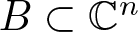
$B\subset \mathbb{C}^n$
Let  $P_a$ be the orthogonal projection of
 $\mathbb{C}^n$ onto the subspace
 $[a]$ generated by
 $a$, and let
 \begin{equation*}Q=Q_a =
I - P_a\end{equation*}
be the projection onto the orthogonal complement of  $[a]$. Explicitly,
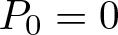 $P_0 = 0$ and
 $P=P_a(z) =\frac{\left \lt z,a\right \gt a}{\left \lt a, a\right \gt }$. Set
 $s_a = (1 - |a|^2)^{1/2}$ and consider the map
 \begin{equation}
p_a(z) =\frac{a-P_a z-s_a Q_a z}{1-\left \lt z,a\right \gt }.
\end{equation}
Compositions of mappings of the form (1.5) and unitary linear mappings of  $\mathbb{C}^n$ constitute the group of holomorphic automorphisms of the unit ball
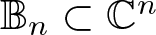 $\mathbb{B}_n\subset \mathbb{C}^n$. It is easy to verify that
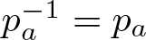 $p_a^{-1}=p_a$. Moreover, for any automorphism
 $q$ of the Bergman ball onto itself, there exists a unitary transformation
 $V$ such that
 \begin{equation}p_{q(c)}\circ q=V\circ p_c.\end{equation}
By using the representation formula [Reference Zhu18, Proposition 1.21], we can introduce the Bergman metric as
 \begin{equation}d_b(z,w)=\frac{1}{2}\log\frac{1+|p_w(z)|}{1-|p_w(z)|}.\end{equation}
If  $\Omega= \{z\in \mathbb{C}^n:\left \lt z,a\right \gt \neq 1\}$, then the map
 $p_a$ is holomorphic in
 $\Omega$. It is clear that
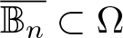 $\overline{\mathbb{B}_n}\subset \Omega$ for
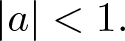 $|a| \lt 1.$
It is well-known that every automorphism  $q$ of the unit ball is an isometry with respect to the Bergman metric, that is:
 $d_b(z,w)=d_b(q(z),q(w))$. In particular, every isometry preserves the volume and perimeter of any measurable subset
 $E\subset \mathbb{B}$ of finite measure.
1.6. Holomorphic barycentre of a set
We know from [Reference Goldman5, p. 54] that the Bergman metric has negative (nonconstant) sectional curvature, which implies that the square of the corresponding distance function is strictly geodesically convex (see [Reference Jost9, eq. 4.8.7]). Consequently, the mapping
 \begin{equation}
K(a) = \int_{E} \log \cosh^2 (d_b(z,a)) (1 - |z|^2)^{-n-1} \, d\upsilon(z)
\end{equation}
is strictly geodesically convex. Therefore, it attains a unique minimum, which we call the holomorphic barycentre of  $E$.
Let  $c$ be the barycentre of
 $E$. Then, the gradient of
 $K(a)$ vanishes at
 $a = c$, leading to the equation
 \begin{equation}
\int_{E} p_c(z) (1 - |z|^2)^{-n-1} \, d\upsilon(z) = 0.
\end{equation}
The barycentre is holomorphically invariant; in other words, if  $\phi$ is any biholomorphic map of the unit ball onto itself and
 $a$ is the barycentre of a set
 $E \subset \mathbb{B}^n$, then
 $\phi(a)$ is the barycentre of the image
 $\phi(E)$. This reflects the natural compatibility of the barycentre with the holomorphic automorphism group of the ball. For further details, we refer the reader to the recent paper [Reference Jacimović and Kalaj8].
Alternatively, one could construct a barycentre using the strict convexity of the function
 \begin{equation*}
H(c) = \int_{E} d^2_b(z,c) (1 - |z|^2)^{-n-1} \, d\upsilon(z),
\end{equation*}
as in [Reference Bögelein, Duzaar and Scheven1]. However, we choose to maintain our definition since the corresponding stationary equation takes a more convenient form.
Including this introduction, the paper consists of four additional sections. In Section 2, we formulate the main results. Section 3 presents auxiliary results necessary for the proofs, which hold for an arbitrary complex dimension  $ n $. In Section 4, we establish a key inequality for the operator
 $ \nabla_{\imath z} $, which appears in the formula for the perimeter. Finally, Section 5 contains the proof of Theorem 2.1.
1.7. Strategy of the proof and the restriction to
$n=2$

The proof follows Fuglede’s perturbative strategy. Firstly, the volume constraint controls the constant spherical harmonic, while the holomorphic barycentre condition controls the first spherical harmonics. The remaining higher modes are controlled through the second-order expansion of the Bergman perimeter. The main additional difficulty, compared with the Euclidean and hyperbolic cases, is the anisotropic factor in the Bergman perimeter formula, which contains the tangential derivative in the Hopf direction  $\imath z$. Most of the preliminary formulae in Section 3 are valid for arbitrary complex dimension
 $n$. The final theorem is stated and proved for
 $n=2$, equivalently for perturbations of
 $\mathbb{S}^3$, because the needed coercive estimate for the operator
 $\nabla_{\imath z}$ is proved here by an explicit eigenmode decomposition on
 $\mathbb{S}^3$. The analogous result is expected in higher complex dimensions once the corresponding spectral estimate is established.
2. The main result
To formulate our main result, let us introduce some notation. Let  $\mathbb{S}$ be the unit sphere in
 $\mathbb{C}^n$. For a given point
 $z \in \mathbb{S}$, the tangent space
 $T_z \mathbb{S}$ is the set of all vectors in
 $\mathbb{C}^n$ that are orthogonal to
 $z$, i.e.,
 \begin{equation*}
T_z \mathbb{S} = \{v \in \mathbb{C}^n : \operatorname{Re}(\langle z, v \rangle) = 0 \},
\end{equation*}
where  $\langle z, v \rangle = \sum_{j=1}^n z_j \overline{v_j}$ is the Hermitian inner product.
Let  $\tau = \{\tau_1, \dots, \tau_{2n-1}\}$ be an orthonormal frame for
 $T_z \mathbb{S}$, consisting of vectors that satisfy:
 \begin{equation*}
\langle \tau_i, \tau_j \rangle = \delta_{ij}, \quad \text{and } \operatorname{Re}(\langle z, \tau_i \rangle) = 0\,\,\text{for all } i.
\end{equation*}
Let  $\nabla$ denote the Levi-Civita connection on the sphere
 $\mathbb{S}$. For any real-valued differentiable function
 $U$ on
 $\mathbb{S}$, the covariant derivative in the direction of
 $\tau_i$ is defined as
 $\nabla_{\tau_i} U$. The notation
 $\nabla_\tau U$ refers to the collection of these covariant derivatives:
 \begin{equation*}
\nabla_\tau U = \{\nabla_{\tau_1} U, \nabla_{\tau_2} U, \dots, \nabla_{\tau_{2n-1}} U \}.
\end{equation*}
The norm of  $\nabla_\tau$ is given by the sum of the squared norms of these directional derivatives:
 \begin{equation*}
|\nabla_\tau U|^2 = \sum_{i=1}^{2n-1} (\nabla_{\tau_i} U)^2.
\end{equation*}
Then we define
 \begin{equation*}\|U\|^2_{W^{1,2}}=\int_{\mathbb{S}}|\nabla_\tau U|^2 d\mathcal{H} + \int_{\mathbb{S}}|U|^2 d\mathcal{H}.\end{equation*}
We also define
 \begin{equation*}\|U\|_{W^{1,\infty}}=\max\{|\nabla_\tau U|_\infty, |U|_\infty\}.\end{equation*}
Theorem 2.1 (Fuglede’s theorem for the Bergman ball)
For any 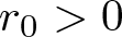 $ r_0 \gt 0 $, there exists a constant
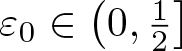 $ \varepsilon_0 \in \left(0, \frac{1}{2} \right] $, depending only on
 $ r_0 $, such that the following holds:
Consider any nearly spherical set  $ E \subset \mathbb{B}_2 $ in the Bergman ball in
 $ \mathbb{C}^2 $, with its barycentre at the origin and satisfying the volume constraint
 \begin{equation*}
\mu (E) = \mu(\mathbb{B}_r),
\end{equation*}
for some 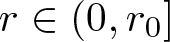 $ r \in (0, r_0] $.
Suppose the boundary of  $ E $ is given by a graph over the unit sphere
 $ \mathbb{S} $, expressed as
 \begin{equation*}
Z : \mathbb{S} \to \partial E, \quad Z(\omega) = \omega \tanh\left(\frac{r}{2} (1 + u(\omega))\right),
\end{equation*}
where  $ u : \mathbb{S} \to \mathbb{R} $ is a Lipschitz function satisfying:
 \begin{equation*}
\|u\|_{W^{1,\infty}(\mathbb{S})} \leq \varepsilon_0.
\end{equation*}
Then, the following estimate holds:
 \begin{equation*}
D(E)=\frac{\delta(E)}{P(\mathbb{B}_r)} = \frac{P(E) - P(\mathbb{B}_r)}{P(\mathbb{B}_r)} \geq c_1(r_0) \|u\|_{W^{1,2}(\mathbb{S})}^2,
\end{equation*}
where 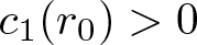 $ c_1( r_0) \gt 0 $ depends only on
 $ r_0 $.
Remark 2.2. We can assume in the previous theorem that 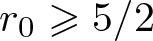 $r_0\geqslant 5/2$. For that
 $r_0$, we can choose
 \begin{equation*}c_1(r_0)=\frac{r_0^2}{8\pi^2 \sinh^2 r_0}.\end{equation*}
3. Auxiliary results
In this section, the integer  $n$, representing the complex dimension of the unit ball, is arbitrary.
3.1. A formula for the volume of
$E$

A parametrization of  $E$ is given by
 \begin{equation*}
\tilde{Z} : \mathbb{S} \times [0, r] \to E, \quad \tilde{Z}(\omega, \rho) = \omega \tanh\left(\frac{\rho}{2} (1 + u(\omega))\right).
\end{equation*}
For a fixed 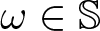 $\omega \in \mathbb{S}$ and
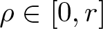 $\rho \in [0, r]$, we introduce the notation
 \begin{equation*}
\mathbf{t} := \tanh\left(\frac{\rho}{2} (1 + u(\omega))\right).
\end{equation*}
Assume that  $\{e_1, \dots, e_{2n}\}$ is a standard orthonormal basis of
 $\mathbb{R}^{2n}$, and let
 $\omega = (\omega_1, \dots, \omega_{2n})$.
To compute the Jacobian of  $\tilde{Z}$, we choose an orthonormal real basis
 $\tau_1, \dots, \tau_{2n-1}$ of
 $T_{\omega} \mathbb{S}$ with respect to the inner product
 \begin{equation*}
\langle w, z \rangle_R := \Re \langle w, z \rangle.
\end{equation*}
In particular, we set
 \begin{equation*}
\tau_{2n-1} = \imath\omega = \imath (\omega_1 + \imath\omega_2, \dots, \omega_{2n-1} + \imath\omega_{2n}) = (-\omega_2, \omega_1, \dots, -\omega_{2n}, \omega_{2n-1}) \in \mathbb{S},
\end{equation*}
and define  $\tau_{2n} = \omega$, ensuring that
 $\langle \omega, \imath\omega \rangle_R = 0$.
Next, we construct an orthonormal basis for  $T_{(\omega, \rho)} (\mathbb{S} \times (0, r))$ as
 \begin{equation*}
(\tau_1, 0), \dots, (\tau_{2n-1}, 0), e_{2n}.
\end{equation*}
Similarly, an orthonormal basis for the tangent space at the point  $X(\omega, \rho)$:
 $T_{X(\omega, \rho)} \mathbb{B}_n \cong \mathbb{R}^{2n}$ is given by
 \begin{equation*}
\tau_1, \dots, \tau_{2n-1}, \omega.
\end{equation*}
Concerning these choices, the Jacobi matrix of  $\tilde{Z}$ reads
 \begin{equation*}
D\tilde{Z}(\omega, \rho) =
\begin{pmatrix}
\mathbf{t} & \cdots & 0 & 0 \\
0 & \cdots & 0 & 0 \\
\vdots & \ddots & \vdots & \vdots \\
0 & \cdots & \mathbf{t} & 0 \\
\frac{\rho(1-\mathbf{t}^2) \partial_1 u}{2} & \cdots & \frac{\rho(1-\mathbf{t}^2) \partial_{2n-1} u}{2} & \frac{1+u}{2}(1-\mathbf{t}^2)
\end{pmatrix} \in \mathbb{R}^{2n \times 2n}.
\end{equation*}
Consequently, the Jacobian of  $\tilde{Z}$ is given by
 \begin{equation}
J\tilde{Z}(\omega, \rho) = \frac{1 + u}{2} \mathbf{t}^{2n-1} (1 - \mathbf{t}^2).
\end{equation}
The volume of  $E$ can thus be written as
 \begin{equation*}
\mu(E) = \int_E \left(1 - |z|^2\right)^{-n-1} d\upsilon(z) = \int_{\mathbb{S}} \int_0^{r} \left(\frac{1}{1 - \mathbf{t}^2}\right)^n \frac{1 + u}{2} \mathbf{t}^{2n-1} \, d\rho \, d\mathcal{H}(\omega).
\end{equation*}
Recalling the definition of  $\mathbf{t}$, we compute
 \begin{equation*}
\left(\frac{1}{1 - \mathbf{t}^2}\right)^n \frac{1 + u(\omega)}{2} \mathbf{t}^{2n-1} = \frac{1+u}{2}\cosh\left[\frac{1}{2} \rho (1+u)\right] \sinh\left[\frac{1}{2} \rho (1+u(\omega))\right]^{2n-1}.
\end{equation*}
So
 \begin{equation*}\begin{aligned}\mu(E) &= \int_{E}\frac{1}{(1-|z|^2)^{n+1}}d\upsilon(z)\\ &=\int_0^{r}\int_{\mathbb{S}}\frac{1+u}{2}\cosh\left[\frac{1}{2} \rho (1+u(\omega))\right] \sinh\left[\frac{1}{2} \rho (1+u(\omega))\right]^{2n-1}d\mathcal{H}(\omega)d\rho
\\ &=\int_{\mathbb{S}}\frac{\sinh^{2n}\left[\frac{1}{2} r (1+u(\omega))\right]}{2n}d\mathcal{H}(\omega).\end{aligned}
\end{equation*}
We recall here that  $d\mathcal{H}=dH^{2n-1}$ is the
 $2n-1$ Hausdorff measure.
3.2. Consequences of the volume constraint
$\mu(\mathbb{B}_r)=\mu (E)$

Let
 \begin{equation*}F(u):=\frac{\sinh^{2n}\left[\frac{1}{2} r (1+u)\right]}{2n}.\end{equation*}
Then
 \begin{equation*}\int_{\mathbb{S}} F(u(\omega))-F(0)d\mathcal{H}(\omega)=0.\end{equation*}
Further
 \begin{equation*}\begin{aligned}
F(u) - F(0) = \frac{1}{4} r \sinh^{2n-2} (\frac{r}{2})\sinh(r) u\\ +\frac{1}{8} r^2 (-1+n+n \cosh r) \sinh^{2n-2}(\frac{r}{2}) u^2+\frac{F'''(u_1)}{6} u^3,
\end{aligned}
\end{equation*}
where
 \begin{equation*}\begin{aligned}F'''(u_1)=\frac{1}{4} r^3 \cosh\left[\frac{1}{2} r (1+u_1)\right] \left(1+(n-3) n+n^2 \cosh[r (1+u_1)]\right)\\ \times \sinh^{2n-3}\left[\frac{1}{2} r (1+u_1)\right].\end{aligned}
\end{equation*}
Note that 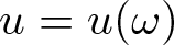 $u=u(\omega)$ and
 $u_1=u_1(\omega)$. Then
 \begin{equation*}\int_{\mathbb{S}} u+\frac{r(-1+n+n \cosh r)}{2 \sinh(r)} u^2+\frac{4F'''(u_1)}{3r \sinh(r)\sinh^{2n-2} (\frac{r}{2})} u^3d\mathcal{H}(\omega)=0.\end{equation*}
Since 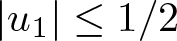 $|u_1|\le 1/2$,
 \begin{equation*}\begin{aligned} \frac{4F'''(u_1)}{6r \sinh(r)\sinh^{2n-2} (\frac{r}{2})}\le C_1(n, r_0), \end{aligned}
\end{equation*}
where
 \begin{equation*}\begin{aligned}C_1(n,r_0)&=\cosh\left[\frac{1}{2} r_0 (1+1/2)\right] \left(1+(n-3) n+n^2 \cosh[r_0 (1+1/2)]\right)\\ &\times \max_{r\in[0,r_0]}\frac{r^2 \sinh^{2n-3}\left[\frac{1}{2} r (1+1/2)\right]}{{6 \sinh(r)\sinh^{2n-2} (\frac{r}{2})} }.\end{aligned}
\end{equation*}
Let
 \begin{equation*}c_0(n,r)=\frac{r}{2 \sinh(r)} (-1+n+n \cosh r).\end{equation*}
It follows that
 \begin{equation}|a_0|=\lvert\int_{\mathbb{S}} u d\mathcal{H}(\omega)\rvert\le c_0(n,r)\int_{\mathbb{S}} u^2 d\mathcal{H}(\omega)+ \varepsilon_0 C_1(n,r_0)\int_{\mathbb{S}} u^2 d\mathcal{H}(\omega).\end{equation}
Since
 \begin{equation*}\int_{\mathbb{S}} u^2 d\mathcal{H}(\omega)= \|u\|_{L^2(\mathbb{S})}^2\le \|u\|_{W^{1,2}}^2\end{equation*}
we obtain that there is a constant 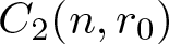 $C_2(n,r_0)$ so that
 \begin{equation}|a_0|\le \varepsilon_0 C_2(n,r_0)\|u\|_{W^{1,2}}.\end{equation}
3.3. Consequence of barycentre constraint
We begin with the following
Remark 3.1. For any point 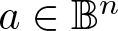 $a \in \mathbb{B}^n$, there exists a biholomorphism
 $\phi_a$ mapping
 $a$ to the origin. So if a domain
 $E$ has barycentre
 $a$, then its image
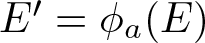 $E'=\phi_a(E)$ has barycentre equal to
 $0$ and has the same Bergman volume and perimeter as
 $E$.
If  $z=0$ is the barycentre, then it follows from (1.8) that
 \begin{equation*}\int_E z (1-|z|^2)^{-1-n} d\upsilon(z)=0.\end{equation*}
Thus, from (3.1) we have
 \begin{equation*} \int_0^{r} \int_{\mathbb{S}}(1-{\mathbf{t}}^2)^{-n-1} \omega \frac{(1+u(\omega))}{2}{\mathbf{t}}^{2n-1}(1-\mathbf{t}^2) \mathbf{t}d\rho d\mathcal{H}(\omega)=0.\end{equation*}
Hence
 \begin{equation*} \int_0^{r} \int_{\mathbb{S}}(1-\mathbf{t}^2)^{-n} \omega \frac{(1+u(\omega))}{2}\mathbf{t}^{2n} d\rho d\mathcal{H}(\omega)=0.\end{equation*}
Thus
 \begin{equation*}\int_0^{r} \int_{\mathbb{S}}\omega(1+u(\omega))\sinh^{2n}\left[\frac{1}{2} \rho (1+u(\omega ))\right]d\rho d\mathcal{H}(\omega)=0.\end{equation*}
Let
 \begin{equation*}\phi(u)=(1+u)\sinh^{2n}\left[\frac{1}{2} \rho (1+u)\right]. \end{equation*}
Since
 \begin{equation*}\int_0^{r} \int_{\mathbb{S}}\omega\sinh^{2n}\left[\frac{1}{2} \rho \right]d\rho d\mathcal{H}(\omega)=0,\end{equation*}
and
 \begin{equation*} \phi(u) = \phi(0)+\phi'(0)u + \frac{\phi''(u_0)}{2!} u^2, \end{equation*}
for some  $u_0=u_0(\omega)\in[-1/2,1/2]$, we get
 \begin{equation*}\int_0^{r} \int_{\mathbb{S}} (\phi'(0)u + \frac{\phi''(u_0)}{2!} u^2)\omega d\rho d\mathcal{H}(\omega)=0.\end{equation*}
Further
 \begin{equation*}\phi'(0)=\sinh \left[\frac{\rho}{2}\right]^{-1+2 n} \left(n \rho \cosh \left[\frac{\rho}{2}\right]+\sinh \left[\frac{\rho}{2}\right]\right)\end{equation*}
and
 \begin{equation*}\begin{aligned}\phi''(u_0)&= \frac{1}{2} n \rho(1+u_0) \sinh \left[\frac{\rho(1+u_0)}{2}\right]^{-2+2 n} \\ & \times(\rho(1+u_0) (-1+n+n \cosh [\rho(1+u_0)])+2 \sinh [\rho(1+u_0)]),\end{aligned}
\end{equation*}
and this implies that
 \begin{equation*}\phi''(u)\le \phi''(1)=n \rho \sinh^{-2+2 n}(\rho) (\rho(-1+n+n \cosh(2 \rho))+\sinh(2\rho)).\end{equation*}
Since
 \begin{equation*}r \sinh(\frac{r}{2})^{2 n} \int_{\mathbb{S}} u \omega d\mathcal{H}(\omega) = -\int_0^{r} \int_{\mathbb{S}}\frac{\phi''(u_0)}{2!} u^2\omega d\rho d\mathcal{H}(\omega),\end{equation*}
we obtain
 \begin{equation*}\begin{aligned}
|r \sinh(\frac{r}{2})^{2 n} \int_{\mathbb{S}} u \omega d\mathcal{H}(\omega)|&\le \int_0^{r} \int_{\mathbb{S}}|\frac{\phi''(1)}{2!} u^2|\omega| d\rho d\mathcal{H}(\omega)
\\ &=\frac{n}{2} r^2 \cosh(r) \sinh^{2n-1}(r) \int_{\mathbb{S}} u^2|\omega| d\rho d\mathcal{H}(\omega).\end{aligned}
\end{equation*}
Thus for  $\omega=(\omega_1,\dots,\omega_{2n})\in \mathbb{S}$ we have for every
 $j$
 \begin{equation}\left|\int_{\mathbb{S}} u \omega_j d\mathcal{H} \right|\le C_3(n,r_0)\varepsilon_0\|u\|_{W^{1,2}(\mathbb{S})}.\end{equation}
3.4. Spherical harmonics and
$W^{1,2}$ norm of
$u$


For any integer  $ k \geq 0 $, let us denote by
 $ \Phi_{k,i}, \, i = 1, \ldots, d_k $, the spherical harmonics of order
 $ k $, i.e., the restriction to
 $ \mathbb{S} $ of the homogeneous harmonic polynomials of degree
 $ k $, normalized such that
 \begin{equation*}
\|\Phi_{k,i}\|_{L^2(\mathbb{S})} = 1, \quad \text{for all } k\,\,\text{and } i \in \{1, \ldots, d_k\}.
\end{equation*}
Here
 \begin{equation}
d_k=\binom{k+2n-1}{k}-\binom{k+2n-3}{k-2}.
\end{equation}
First of all
 \begin{equation*}
\int_{\mathbb{S}} 1 \, d\mathcal{H} = \Omega_n,
\end{equation*}
where  $ \Omega_n $ is the
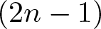 $ (2n-1) $-dimensional measure of the unit sphere
 $ \mathbb{S} $. For
 $ i = 1, \ldots, n $, for
 $z=(x_1+iy_1,\dots, x_n+i y_n)$ it follows that
 \begin{equation*}
\int_{\mathbb{S}} x_i^2 \, d\mathcal{H} =\int_{\mathbb{S}} y_i^2 \, d\mathcal{H}= \frac{1}{2n} \int_{\mathbb{S}} |z|^2 \, d\mathcal{H} = \frac{\Omega_n}{2n}.
\end{equation*}
Hence, we have
 \begin{equation*}
\Phi_{0,0} = \frac{1}{\sqrt{\Omega_n}} \quad \text{and} \quad \Phi_{1,i} = \sqrt{\frac{2n}{\Omega_n}}\,x_i, \quad \Phi_{1,i+n} = \sqrt{\frac{2n}{\Omega_n}}\,y_i
\end{equation*}
respectively.
The functions  $ \Phi_{k,i} $ are eigenfunctions of the Laplace-Beltrami operator on
 $ \mathbb{S} $. Specifically, for all
 $ k $ and
 $ i $,
 \begin{equation*}
-\Delta_{\mathbb{S}} \Phi_{k,i} = k(k + 2n - 2) \Phi_{k,i}.
\end{equation*}
Therefore, if we write
 \begin{equation*}
u = \sum_{k=0}^\infty \sum_{i=1}^{d_k} a_{k,i} \Phi_{k,i}, \quad \text{where} \quad a_{k,i} = \int_{\mathbb{S}} u \Phi_{k,i} d\mathcal{H},
\end{equation*}
we have
 \begin{equation*}
\|u\|_{L^2(\mathbb{S})}^2 = \sum_{k=0}^\infty \sum_{i=1}^{d_k} a_{k,i}^2.
\end{equation*}
Further
 \begin{equation*}
\int_{\mathbb{S}} |\nabla u|^2 \, d\mathcal{H}
= -\int_{\mathbb{S}} u \, \Delta_{\mathbb{S}} u \, d\mathcal{H}
= \sum_{k=1}^\infty \sum_{i=1}^{d_k} k(k + 2n - 2)a_{k,i}^2.
\end{equation*}
We therefore have
 \begin{equation}
\|\nabla u\|^2_{L^2 (\mathbb{S})} = \sum_{k=0}^\infty \sum_{i=1}^{d_k} \big[k(k + 2n - 2)\big]a_{k,i}^2
\end{equation}
and
 \begin{equation}
\|u\|_{W^{1,2}}^2 = \sum_{k=0}^\infty \sum_{i=1}^{d_k} \big[k(k + 2n - 2) + 1\big]a_{k,i}^2.
\end{equation}
It follows from (3.4) that
 \begin{equation}\left|a_{1,i}\right|\le C_3(n,r_0)\varepsilon_0\|u\|_{W^{1,2}(\mathbb{S})}, i=1,\dots, 2n.\end{equation}
3.5. Formula for the perimeter
Let
 \begin{equation*}
\mathbf t=\tanh\left(\frac r2(1+u(\omega))\right),\qquad
\mathbf t_0=\tanh\frac r2.
\end{equation*}
For 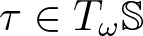 $\tau\in T_\omega\mathbb S$,
 \begin{equation*}
d_\omega Z(\tau)
=\mathbf t\,\tau+\frac{r(1-\mathbf t^2)}{2}\,D_\tau u\,\omega .
\end{equation*}
Therefore, by the rank-one determinant formula,
 \begin{equation*}
JZ(\omega)
=\mathbf t^{2n-1}
\left[1+\left(\frac{1-\mathbf t^2}{2\mathbf t}\right)^2r^2|\nabla_\tau u|^2\right]^{1/2}.
\end{equation*}
Let  $E_1=\partial E=\{z:U(z)=r\}$. By (1.3),
 \begin{equation}
P(E_1)=\int_{E_1}d\tilde\sigma(z)=\int_{\mathbb S}Z_*(d\tilde\sigma),
\end{equation}
where
 \begin{equation*}
d\tilde\sigma(z)=
(1-|z|^2)^{-n-\frac12}
\sqrt{1-\frac{|\langle\nabla U,z\rangle|^2}{|\nabla U|^2}}\,d\sigma(z).
\end{equation*}
Thus
 \begin{equation}
Z_*(d\tilde\sigma)
=\frac{\mathbf t^{2n-1}}{(1-\mathbf t^2)^{n+1/2}}
\sqrt{1-\frac{|\langle\nabla U,z\rangle|^2}{|\nabla U|^2}}
\left[1+\left(\frac{1-\mathbf t^2}{2\mathbf t}\right)^2r^2|\nabla_\tau u|^2\right]^{1/2}d\mathcal H(\omega).
\end{equation}
Let
 \begin{equation*}
U(z)=\frac{2\tanh^{-1}|z|}{1+u(z/|z|)},\qquad z\neq0.
\end{equation*}
Then
 \begin{equation*}
E=\{z\in\mathbb C^n:U(z) \lt r\},\qquad
\partial E=\{z\in\mathbb C^n:U(z)=r\}
=\{Z(\omega):\omega\in\mathbb S\},
\end{equation*}
where
 \begin{equation*}
Z(\omega)=\omega\tanh\left(\frac r2(1+u(\omega))\right).
\end{equation*}
For vectors  $\tau_k$ as in Subsection 3.1,
 \begin{equation*}
\nabla_{\tau_k}U(z)=\frac{-2\nabla_{\tau_k}u}{(1+u(\omega))^2}\tanh^{-1}|z|,
\qquad
\nabla_{\mathbf n}U(z)=\frac{2}{(1-|z|^2)(1+u(\omega))},
\end{equation*}
where 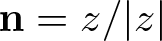 $\mathbf n=z/|z|$. In the sequel, we use the complex inner product
 $\langle\cdot,\cdot\rangle$ and the real inner product
 $\langle\cdot,\cdot\rangle_R=\operatorname{Re}\langle\cdot,\cdot\rangle$. Choosing the frame so that
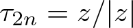 $\tau_{2n}=z/|z|$ and
 $\tau_{2n-1}=\imath z/|z|$, we get
 \begin{equation}
|\langle z,\nabla U\rangle|
=|z|\sqrt{|\partial_{\mathbf n}U|^2+|\partial_{\tau_{2n-1}}U|^2},
\end{equation}
and
 \begin{equation}
|\nabla U|^2=|\partial_{\mathbf n}U|^2+|\nabla_\tau U|^2
=|\partial_{\mathbf n}U|^2+\sum_{k=1}^{2n-1}|\partial_{\tau_k}U|^2.
\end{equation}
Let us introduce the shorthand notation for the sequel
 \begin{equation*}\mathbf{t}=\tanh[r/2(1+u(\omega))],\end{equation*}
 \begin{equation*}R=\frac{\left(\frac{1+u(\omega)}{1-\mathbf{t}^2}\right)^2}{(\tanh^{-1}(\mathbf{t}))^2}=\frac{4}{r^2 \left(1-\mathbf{t}^2\right)^2 }\end{equation*}
and
 \begin{equation*}x=|\nabla_\tau u|^2,\qquad s=|\nabla_{\tau_{2n-1}}u|^2.\end{equation*}
Let
 \begin{equation*}h(x)={\sqrt{1+\frac{r^2 \left(1-\mathbf{t}^2\right)^2 x}{4\mathbf{t}^2}}} \end{equation*}
and
 \begin{equation*}k(x,s)=\sqrt{1-\frac{\mathbf{t}^2 (R+s)}{R+ x}}.\end{equation*}
(a) By using the elementary inequality
 \begin{equation*}\sqrt{1+y}\geqslant 1+\frac{y}{2}-\frac{y^2}{8},\end{equation*}
by making the substitution  $\mathbf{t}=\tanh(\frac{r}{2}(1+u))$ we obtain
 \begin{equation*}h(x)\geqslant 1+\frac{1}{2} r^2 \operatorname{csch}^2(r (1+u)) x-\frac{1}{8} \left(r^4 \operatorname{csch}^4(r (1+u))\right) x^2.\end{equation*}
By using continuity and the fact that  $|u|\le \varepsilon_0 \lt 1/2$ for
 $r\le r_0$ we obtain,
 \begin{equation}h(x) \geqslant 1+ \frac{1}{2} x r^2 \operatorname{csch}^2 r - \varepsilon_0 C_{4}(n,r_0) x.\end{equation}
(b) Now consider
 \begin{equation*}k(x,s)=\frac{\sqrt{1-\frac{(R+s) \mathbf{t}^2}{R+ x}}}{\sqrt{1-\mathbf{t}^2}}.\end{equation*}
Then
 \begin{equation*}k(x,s) = h(x,s)+s^2\mathbf{r_1}\end{equation*}
where
 \begin{equation*} h(x,s)=\frac{\sqrt{1-\frac{R \mathbf{t}^2}{R+x}}}{\sqrt{1-\mathbf{t}^2}}-\frac{\mathbf{t}^2 s}{2 \left(\sqrt{1-\mathbf{t}^2} (R+x) \sqrt{1-\frac{R \mathbf{t}^2}{R+x}}\right)}\end{equation*}
and
 \begin{equation*}\mathbf{r_1}=-\frac{\mathbf{t}^4}{8 \sqrt{1-\mathbf{t}^2} (R+x)^2 \left(1-\frac{(R+s_1) \mathbf{t}^2}{R+x}\right)^{3/2}},\end{equation*}
and  $s_1\in [0,1/2]$. Given the definition of
 $R$ and
 $\mathbf{t}\le \tanh(r_0)$, we obtain that
 \begin{equation*}|\mathbf{r_1}|\le C_4(n,r_0).\end{equation*}
Further
 \begin{equation*}h(x,s)= 1+\frac{\mathbf{t}^2 (x-s)}{2 R \left(1-\mathbf{t}^2\right)}-\frac{s \mathbf{t}^2 \left(2-\mathbf{t}^2\right) x}{4 R^2 \left(1-\mathbf{t}^2\right)^2}+ \mathbf{r_2} x^2 \end{equation*}
where
 \begin{equation*}\begin{aligned}\mathbf{r_2}&=\frac{R^2 \mathbf{t}^4 \left(-3 s \mathbf{t}^2+2 R \left(-1+\mathbf{t}^2\right)-2 x\right)}{16 \sqrt{1-\mathbf{t}^2} (R+x)^5 \left(1-\frac{R \mathbf{t}^2}{R+x}\right)^{5/2}}
\\ &- \frac{\mathbf{t}^2 \left(R^2 \left(1-\mathbf{t}^2\right)+s x+R (s+x)\right)}{2\sqrt{1-\mathbf{t}^2} \left(R \left(1-\mathbf{t}^2\right)+x\right) (R+x)^3 \sqrt{1-\frac{R \mathbf{t}^2}{R+x}}}.\end{aligned}
\end{equation*}
Since
 \begin{equation*}R\geqslant \frac{4}{r_0^2(1-\tanh(r_0)^2)}, \end{equation*}
 \begin{equation*}\mathbf{t}\le \tanh(r_0),\ \ \ \ 0\le s\le x\le 1/2\end{equation*}
and  $\lim_{R\to +\infty } \mathbf{r_2}=0$. It follows that there is a constant
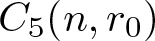 $C_5(n,r_0)$ so that
 \begin{equation*}|\mathbf{r_2}|\le C_5(n,r_0).\end{equation*}
Using the condition  $\|u\|_{W^{1,\infty}}\le \varepsilon_0$, we obtain that there is a constant
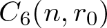 $C_6(n,r_0)$ so that
 \begin{equation}
k(x,s)\geqslant 1+ \frac{r^2}{8} \tanh^2(\frac{r}{2})\left(1-\tanh^2(\frac{r}{2})\right)(x-s) - C_6(n,r_0)\varepsilon_0 x.\end{equation}
By using the equation
 \begin{equation*}{\sqrt{1-\frac{|\left \lt \nabla U, z\right \gt |^2}{|\nabla U|^2}}}=\sqrt{1-|z|^2 \frac{|\partial_{\mathbf{n}} U|^2 + |\nabla_{\tau_{2n-1}} U|^2}{|\partial_{\mathbf{n}} U|^2 + |\nabla_\tau U|^2}}\end{equation*}
and (3.13) and (3.14), we have
Lemma 3.2. Under previous notation, if  $0 \lt r \lt r_0$ and
 $\|u\|_{W^{1,\infty}} \lt \varepsilon_0$ then
 \begin{equation*}\begin{aligned}{\sqrt{1-\frac{|\left \lt \nabla U, z\right \gt |^2}{|\nabla U|^2}}}&\left[ 1 + \left( \frac{1 - \mathbf{t}^2}{2\mathbf{t}} \right)^2 r^2 |\nabla_\tau u|^2 \right]^{1/2}
\\ &\geqslant 1+\frac{1}{2} r^2 \operatorname{csch}^2 r |\nabla_\tau u|^2\\ &+\frac{1}{8} r^2 \tanh^2(\frac{r}{2})(1-\tanh^2(\frac{r}{2}))(|\nabla_\tau u|^2-|\nabla_{\tau_{2n-1}} u|^2) \\ &-\varepsilon_0 C_{8}(n,r_0)|\nabla_\tau u|^2.\end{aligned}
\end{equation*}
4. A spectral estimate for
$\nabla_{\imath z}$ on
$\mathbb{S}^3$


The aim of this section is to prove the following lemma
Lemma 4.1. Assume that  $U\in W^{1,2}(\mathbb{S}^3)$ and let
 \begin{equation*}U(z) = \sum_{k=0}^\infty \sum_{j=1}^{d_k} a_{k,j} \Phi_{k,j}(z),\end{equation*}
where  $\Phi_{k,j}$ is an orthonormal basis of spherical harmonics that solves the Laplace equation
 $\Delta_{\mathbb{S}} \Phi=-k(k+2) \Phi$ of the unit norm. Then
 \begin{equation}
\|\nabla U\|^2_{L^2(\mathbb{S})}-\|\left \lt \nabla U, \imath z\right \gt \|^2_{L^2(\mathbb{S})}\geqslant 2\sum_{k=0}^\infty\sum_{j=1}^{d_k} ka^2_{k,j}.
\end{equation}
Proof. Let us extend  $U$ in
 $\mathbb{B}^4\setminus{0}$ so that
 $U(z) = U(z/|z|)$ and let us consider the (Hopf) coordinates
 $z=J(r,t,s,\varphi)=(x,y,u,v)$, where
 \begin{equation*}x=r \cos s \cos t, \ \ \ y=r \cos s \sin t;\end{equation*}
 \begin{equation*}u=r \sin s \cos \varphi ;v=r \sin s \sin \varphi.\end{equation*}
Here  $t,\varphi\in[0,2\pi]$ and
 $s\in[0,\pi/2]$. In complex notation
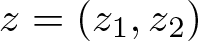 $z=(z_1,z_2)$, where
 $z_1=r \cos s e^{\imath t}$ and
 $z_2=r \sin s e^{\imath \varphi}$.
Then
 \begin{equation*}A=(\left(DJ(r,s,t,\varphi)\right)^{-1})^T=
\begin{bmatrix}
\cos s \cos t & -\frac{\cos t \sin s}{r} & -\frac{\sec s \sin t}{r} & 0 \\
\cos s \sin t & -\frac{\sin s \sin t}{r} & \frac{\cos t \sec s}{r} & 0 \\
\cos \varphi \sin s & \frac{\cos \varphi \cos s}{r} & 0 & -\frac{\csc s \sin \varphi}{r} \\
\sin \varphi \sin s & \frac{\cos s \sin \varphi}{r} & 0 & \frac{\cos \varphi \csc s}{r}
\end{bmatrix}
\end{equation*}
and
 \begin{equation*}\begin{aligned}\nabla U&=A(U_r,U_s,U_t,U_\varphi)\\ &=
\begin{bmatrix}
U_r \cos s \cos t - U_s \cos t \sin s - U_t \sec s \sin t \\
U_t \cos t \sec s + (U_r \cos s - U_s \sin s) \sin t \\
-U_\varphi \csc s \sin \varphi + \cos \varphi (U_s \cos s + U_r \sin s) \\
U_\varphi \cos \varphi \csc s + \sin \varphi (U_s \cos s + U_r \sin s)
\end{bmatrix}.
\end{aligned}
\end{equation*}
Moreover 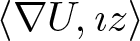 $\left \lt \nabla U, \imath z\right \gt $ is equal to the expression
 \begin{equation*}
-y \, U_x + x \, U_y - v \, U_u + u \, U_v
\end{equation*}
which simplifies to:
 \begin{equation}
\left\langle \nabla U, \imath z \right\rangle = \frac{\partial U}{\partial t} + \frac{\partial U}{\partial \varphi}.
\end{equation}
Similarly, we can find 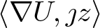 $\left \lt \nabla U, \jmath z\right \gt $ and
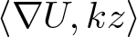 $\left \lt \nabla U, k z\right \gt $, where
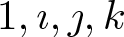 $1,\imath,\jmath,k$ are quaternions on
 $\mathbb{R}^4$. Then we get
 \begin{equation*}|\nabla U|^2 =\left \lt \nabla U, \imath z\right \gt ^2+\left \lt \nabla U, \jmath z\right \gt ^2+\left \lt \nabla U, k z\right \gt ^2= U_s^2+\frac{U_t^2}{\cos^2 s}+\frac{U_\varphi^2}{\sin^2 s}.\end{equation*}
Assume that 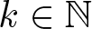 $k\in \mathbb{N}$ and let
 $m,\ell\in \{-k,\dots, k\}$ satisfying the condition
 $(m+\ell)=k\mod 2$. The so-called eigenmode (see [Reference Lachièze-Rey12, Reference Lehoucq, Uzan and Weeks14]) is defined by:
 \begin{equation*}
\widetilde{\Psi}_{k\ell m}(s,t,\varphi) = \cos^{|\ell|}s\,\sin^{|m|}s\,P_{d}^{(|m|,|\ell|)}(\cos 2s)
\end{equation*}
 \begin{equation*}
\times (\cos|\ell|t\quad\text{or}\quad\sin|\ell|t)
\end{equation*}
 \begin{equation*}
\times (\cos|m|\varphi\quad\text{or}\quad\sin|m|\varphi)
\end{equation*}
where the choice of  $\cos|\ell|t$ or
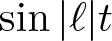 $\sin|\ell|t$ (resp.
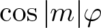 $\cos|m|\varphi$ or
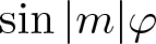 $\sin|m|\varphi$) depends on the sign of
 $\ell$ (resp.
 $m$). Here
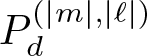 $ P_d^{(|m|, |\ell|)} $ is the Jacobi polynomial
 \begin{equation*}
P_d^{(|m|, |\ell|)}(u) = \frac{1}{2^d} \sum_{i=0}^d \binom{|m| + d}{i} \binom{|\ell| + d}{d - i} (u + 1)^i (u - 1)^{d-i}
\end{equation*}
and
 \begin{equation*}
d = \frac{k - (|\ell| + |m|)}{2}.
\end{equation*}
Define the normalized eigenmodes  $\Psi_{k\ell m}$ by
 \begin{equation*}
\Psi_{k\ell m} = \frac{\widetilde{\Psi}_{k\ell m}}{\sqrt{\langle\widetilde{\Psi}_{k \ell m},\widetilde{\Psi}_{k\ell m}\rangle}} = \frac{\widetilde{\Psi}_{k\ell m}}{\sqrt{2^{\hat{\ell}+\hat{m}}} \ \pi \ \sqrt{\frac{(|\ell|+d)!}{2(k+1)}\ d! \ (|\ell|+|m|+d)!}}
\end{equation*}
where  $\hat{\ell}$ is 1 when
 $\ell$ is 0, and
 $\hat{\ell}$ is 0 when
 $\ell$ is nonzero, and similarly for
 $\hat{m}$. Now we need the following proposition
Proposition 4.2. ([Reference Lehoucq, Uzan and Weeks14, Theorem 1])
The functions  $\Psi_{k\ell m}$, indexed by all integers
 $k$,
 $\ell$, and
 $m$ satisfying the conditions
 $|\ell| + |m| \leq k$ and
 $\ell + m \equiv k \pmod{2}$, form an orthonormal basis for the eigenspace of the Laplacian on the 3-sphere. Let
 $ I(k) $ denote the set of valid index pairs
 $(\ell, m)$ for a given
 $k$. Furthermore, these functions satisfy the eigenvalue equation
 \begin{equation*}
-\Delta_{\mathbb{S}} \Psi_{k\ell m} = k(k+2) \Psi_{k\ell m}.
\end{equation*}
Since  $|I(k)|=d_k=(1+k)^2$ (by (3.5)), we have
 $I(k)=\{i_1,i_2,\dots, i_{d_k}\}.$ Now if
 $U\in L^2(\mathbb{S})$, then we have
 \begin{equation} U(z)=\sum_{k\in \mathbb{N}_0}\sum_{(\ell, m)\in I(k)} \tilde a_{k,\ell,m} \Psi_{k\ell m}=\sum_{k=0}^\infty \sum_{j=1}^{d_k}a_{k,j}\Phi_{k,j},\end{equation}
where 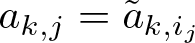 $a_{k,j}=\tilde a_{k, i_j}$, and
 $\Phi_{k,j}=\Psi_{k, i_j}$, and
 \begin{equation*}\|U\|^2_{L^2(\mathbb{S})}=\sum_{k,\ell, m} \tilde a^2_{k,\ell,m} .\end{equation*}
Here  $i_j$ is a certain pair
 $(\ell,m)$ from
 $I_k$. Moreover
 \begin{equation*} \|\nabla U\|^2_{L^2(\mathbb{S})} =\sum_{k,\ell, m} k(k+2)\tilde a^2_{k,\ell,m}\end{equation*}
and
 \begin{equation*}\begin{aligned}\left \lt \nabla U, \imath z\right \gt &=\sum_{k,\ell, m} \tilde a_{k,\ell,m} \left \lt \Psi_{k\ell m}, \imath z\right \gt \\ &= \sum_{k,\ell, m} \tilde a_{k,\ell,m} \left(\frac{\partial \Psi_{k\ell m}}{\partial t}+\frac{\partial \Psi_{k\ell m}}{\partial \varphi}\right).\end{aligned}
\end{equation*}
Since the angular part of  $\Psi_{k\ell m}$ is a product of a trigonometric mode of frequency
 $|\ell|$ in
 $t$ and a trigonometric mode of frequency
 $|m|$ in
 $\varphi$, orthogonality of the trigonometric modes gives
 \begin{equation*}
\left\|\left(\frac{\partial}{\partial t}+\frac{\partial}{\partial\varphi}\right)
\Psi_{k\ell m}\right\|_{L^2(\mathbb S)}^2=\ell^2+m^2.
\end{equation*}
Moreover, the functions
 \begin{equation*}
\left(\frac{\partial}{\partial t}+\frac{\partial}{\partial\varphi}\right)
\Psi_{k\ell m}
\end{equation*}
are mutually orthogonal for distinct triples 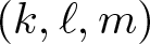 $(k,\ell,m)$.
Thus
 \begin{equation}\|\left \lt \nabla U, \imath z\right \gt \|^2_{L^2(\mathbb{S})}= \sum_{k\in \mathbb{N},(\ell, m)\in I(k)} (m^2+\ell^2)\tilde a^2_{k,\ell,m} \le \sum_{k=0}^\infty\sum_{j=1}^{d_k} k^2a^2_{k,j},\end{equation}
where  $\tilde a_{k,\ell,m}=a_{k,j}$ provided that
 $(\ell, m)$ corresponds to
 $j$ as in (4.3).
Therefore, in view of Proposition 4.2, from (3.6) and (4.4), the proof of Lemma 4.1 is completed.
5. Proof of the main result
Proof of Theorem 2.1
Unlike Section 3, where  $n$ was arbitrary, in this proof, we set
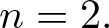 $n=2.$ Let
 \begin{equation}G(r,\omega)=\frac{1}{2} r^2 \operatorname{csch}^2 r |\nabla_\tau u|^2+\frac{1}{8} r^2 \tanh^2(\frac{r}{2})(1-\tanh^2(\frac{r}{2}))(|\nabla_\tau u|^2-|\nabla_{\tau_{3}} u|^2)\end{equation}
and
 \begin{equation*}\mathbf{t}_\circ=\tanh\left(\frac{r}{2}\right).\end{equation*}
 \begin{equation*}P(E)-P(\mathbb{B}_r)\geqslant \int_{\mathbb{S}}\mathbf{t}^{3}(1-\mathbf{t}^2)^{-2}\left(G(r,\omega)- \varepsilon_0 C_{8}(r_0) |\nabla_\tau u|^2\right) d\mathcal{H}\end{equation*}
 \begin{equation*} + \int_{\mathbb{S}}\mathbf{t}^{3}(1-\mathbf{t}^2)^{-2}-\mathbf{t}_\circ^{3}(1-\mathbf{t}_\circ^2)^{-2}d\mathcal{H}.\end{equation*}
Further, let
 \begin{equation*}M(u):= \left( \frac{\sinh\left[\frac{1}{2} r (1+u)\right]}{\sinh \frac{r}{2}}\right)^{2 } \frac{\sinh[r (1+u)]}{\sinh(r)}-1.\end{equation*}
Then
 \begin{equation}
\begin{aligned}
M(u)&=\frac{\mathbf{t}^{3} (1-\mathbf{t}^2)^{-2}}{\mathbf{t}_\circ^{3} (1-\mathbf{t}_\circ^2)^{-2}} - 1
\\ &= \, r \left( 1+ 2 \cosh(r) \right) \operatorname{csch}(r) \, u \\
& + \frac{1}{4} r^2 \left( -1 + 4 \cosh(r) \right)
\operatorname{csch}\left( \frac{r}{2} \right)^2 u^2 \\
& + R(w) u^3,
\end{aligned}
\end{equation}
where
 \begin{equation*}\begin{aligned}
R(w)=\frac{1}{6}M'''(w)\\ =-\frac{r^3 (\cosh[r (1+w)]-4 \cosh[2 r (1+w)])}{3 (-2 \sinh r+\sinh(2 r))} \end{aligned}
\end{equation*}
and  $w\in[-1/2,1/2]$. Moreover
 \begin{equation}R(w) u^3\geqslant - C_{9}(r_0)\varepsilon_0 |u|^2.\end{equation}
From (5.2) and (5.3), we immediately get that
 \begin{equation}\frac{\mathbf{t}^{3} (1-\mathbf{t}^2)^{-2}}{\mathbf{t}_\circ^{3} (1-\mathbf{t}_\circ^2)^{-2}} \geqslant 1- C_7(r_0)\varepsilon_0.\end{equation}
Then
 \begin{equation*}\begin{aligned}
\frac{P(E)-P(\mathbb{B}_r)}{{\mathbf{t}_\circ^{3} (1-\mathbf{t}_\circ^2)^{-2}}} &=I_1+I_2
\\ &=\int_{\mathbb{S}}\frac{\mathbf{t}^{3}(1-\mathbf{t}^2)^{-2}}{{{\mathbf{t}_\circ^{3} (1-\mathbf{t}_\circ^2)^{-2}}}}\left(G(r,\omega) - C_{8}(r_0)\varepsilon_0 |\nabla_\tau u|^2\right) d\mathcal{H}
\\ &+ \int_{\mathbb{S}}\left(\frac{\mathbf{t}^{3}(1-\mathbf{t}^2)^{-2}}{\mathbf{t}_\circ^{3}(1-\mathbf{t}_\circ^2)^{-2}}-1\right)d\mathcal{H}.\end{aligned}
\end{equation*}
Now, from (5.4), we have
 \begin{equation*}I_1\geqslant \int_{\mathbb{S}} \left(G(r,\omega) - C_8(r_0)\varepsilon_0 |\nabla_\tau u|^2\right) d\mathcal{H}.\end{equation*}
 \begin{equation*}\begin{aligned}
\frac{1}{4} r^2 &\left(1+(-3+n) n+n^2 \cosh(r)\right) \operatorname{csch}^2(\frac{r}{2})-\frac{1}{2} r^2 (1+2 \cosh r)^2 \operatorname{csch}^2 r
\\ &= -\frac{1}{2} r^2 (2+ \cosh(r)) \operatorname{csch}^2 r,\end{aligned}
\end{equation*}
we obtain
 \begin{equation*}\begin{aligned}I_2&=\int_{\mathbb{S}}\left(\frac{\mathbf{t}^{3}(1-\mathbf{t}^2)^{-2}}{\mathbf{t}_\circ^{3}(1-\mathbf{t}_\circ^2)^{-2}}-1\right)d\mathcal{H}
\\ &\geqslant -c_0(r)\int_{\mathbb{S}} u^2 d\mathcal{H}- C_9(r_0)\varepsilon_0\int_{\mathbb{S}} u^2 d\mathcal{H},\end{aligned}
\end{equation*}
where
 \begin{equation*}c_0(r)=\frac{1}{2} r^2 (2+ \cosh r) \operatorname{csch}^2 r.\end{equation*}
From (4.1)
 \begin{equation*}\int_{\mathbb{S}}(|\nabla_\tau u|^2-|\nabla_{\tau_{3} }u|^2) d\mathcal{H}(\omega)\geqslant 2 \sum_{k=2}^\infty \sum_{i=1}^{d_k} k a^2_{k,i}.\end{equation*}
Since
 \begin{equation*}\frac{1}{2} k (2+k) r^2 \operatorname{csch}^2(r)+\frac{k(2n-2)}{8} r^2 \tanh^2(\frac{r}{2}) \left(1-\tanh^2(\frac{r}{2})\right),\end{equation*}
 \begin{equation*}=\frac{k r^2 (2 k+7 +2 k \cosh(r)+ \cosh(2 r)) \operatorname{csch}^2(r)}{4 (1+\cosh(r))} \end{equation*}
we get
 \begin{equation*}I_1\geqslant \sum_{k\geqslant 2, 1\le i\le d_k} \frac{k r^2 (2 k+7 +2 k \cosh(r)+ \cosh(2 r)) \operatorname{csch}^2(r)}{4 (1+\cosh(r))} a^2_{k,i}\end{equation*}
 \begin{equation*}-C_8(r_0)\varepsilon_0 \int_{\mathbb{S}}|\nabla_\tau u|^2 d\mathcal{H}.\end{equation*}
Since
 \begin{equation*} \frac{k r^2 (2 k+7+2 k \cosh(r)+ \cosh(2r) ) \operatorname{csch}^2(r)}{4 (1+\cosh(r))}-c_0(r)=K(k,r)\end{equation*}
where
 \begin{equation*}K(k,r)=\frac{r^2}{\sinh^2 r} \left((1+k) (k-2)+ \left((-1+k) \cosh(r)+\frac{4 k}{1+\cosh(r)}\right)\right) \end{equation*}
we obtain
 \begin{equation}\begin{aligned}
I_1+I_2&\geqslant \sum_{k\geqslant 2, 1\le i\le d_k}K(k,r) a^2_{k,i}\\ &-c_0(r)(a_{0,0}^2 +\sum_{i=1}^{4} a_{1,i}^2) -C_{10}(r_0)\varepsilon_0\|u\|^2_{W^{1,2}}.\end{aligned}
\end{equation}
We aim to show that for  $k\geqslant 2$ and
 $n\geqslant 2$
 \begin{equation*} K(k,r)\geqslant A (k(k+2)+1)\end{equation*}
with a positive constant  $A$. Let
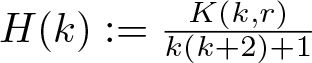 $H(k):= \frac{K(k,r)}{k(k+2)+1}$.
For  $k=2$, we have that
 \begin{equation*} H(k)=A_0(r)=\frac{1}{288} r^2 (17+2 \cosh(r)+\cosh(2 r)) \operatorname{csch}^2(\frac{r}{2}) \mathrm{sech}^4(\frac{r}{2}) \end{equation*}
and
 \begin{equation*}\lim_{k\to \infty} H(k)=A_1(r)=\frac{1}{2} r^2 \operatorname{csch}^2(r).\end{equation*}
Then we have
 \begin{equation*}H'(k)=-\frac{r^2 \left(-7+k-2 (3+k) \cosh(r)+(-3+k) \cosh^2(r)\right) \operatorname{csch}^2(r)}{2 (1+k)^3 (1+\cosh(r))},\end{equation*}
whose only stationary point is
 \begin{equation*}k=k_\circ=\frac{1}{8} (17+12 \cosh(r)+3 \cosh(2r)) \operatorname{csch}^4(\frac{r}{2}).\end{equation*}
In this case
 \begin{equation*}H''(k_\circ)= -\frac{32 r^2 \operatorname{csch}^4 r \sinh^{18}(\frac{r}{2})}{(5+2 \cosh(r)+\cosh(2 r))^3} \lt 0.\end{equation*}
Thus, 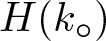 $H(k_\circ)$ is the maximum of
 $H$.
Let  $B_2=\tanh^{-1}\left[2 \sqrt{2 \left(-4+\sqrt{17}\right)}\right]$. Then
 \begin{equation*}A=\min_{r\in[0,r_0]} \{A_0, A_1\}=\min\{A_0(r_0), A_1(r_0)\}=\left\{
\begin{array}{ll}
A_0(r_0), & \hbox{if}\ r_0\le B_2 \\
A_1(r_0), & \hbox{for}\ r_0 \gt B_2.
\end{array}
\right.
\end{equation*}
Let us now prove that
 \begin{equation}
c(r_0)=\max_{0\le r\le r_0}c(r),
\end{equation}
where
 \begin{equation*}
c(r)=\frac{r}{2\sinh r}(1+2\cosh r).
\end{equation*}
Set  $s=\cosh r\geqslant1$. The sign of
 $c'(r)$ is the sign of
 \begin{equation*}
\Psi(s)=(1+2s)\sqrt{s^2-1}-(2+s)\operatorname{arccosh}s.
\end{equation*}
Since  $\Psi(1)=0$ and
 \begin{equation*}
\Psi'(s)=\frac{(7+2s)\sqrt{s^2-1}}{(2+s)^2}\geqslant0,
\end{equation*}
we have 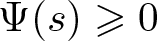 $\Psi(s)\geqslant0$ for
 $s\geqslant1$. Hence,
 $c$ is increasing, and (5.6) follows.
For 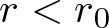 $r \lt r_0$, we now have that
 \begin{equation*}
I_1 + I_2 \geq A \|u\|^2_{W^{1,2}}-A(a_{0,0}^2 +4\sum_{i=1}^{4} a_{1,i}^2) -c_0(r)(a_{0,0}^2 +\sum_{i=1}^{4} a_{1,i}^2) -C_{10}(r_0)\varepsilon_0\|u\|^2_{W^{1,2}}.
\end{equation*}
Now, because of (3.3) and (3.8)
 \begin{equation*}-A(a_{0,0}^2 +4\sum_{i=1}^{4} a_{1,i}^2) -c_0(r)(a_{0,0}^2 +\sum_{i=1}^{4} a_{1,i}^2) -C_{10}(r_0)\varepsilon_0\|u\|^2_{W^{1,2}}\end{equation*}
 \begin{equation*}\geqslant -C_{11}(r_0)\varepsilon_0 \|u\|^2_{W^{1,2}},\end{equation*}
and thus for small enough  $\varepsilon_0$,
 \begin{equation*}
I_1 + I_2 \geq \frac{A}{2} \|u\|^2_{W^{1,2}}.
\end{equation*}
We conclude that if  $\|u\|_{W^{1,\infty}} \lt \varepsilon_0$, and if
 $\varepsilon_0$ is small enough, then
 \begin{equation*}
D(E)=\frac{\delta(E)}{P(\mathbb{B}_r)} = \frac{I_1 + I_2}{\omega_2} \geq C(r_0)\|u\|^2_{W^{1,2}},
\end{equation*}
where
 \begin{equation}C(r_0)=\frac{A}{2\omega_2}.\end{equation}
Here 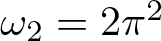 $\omega_2 = 2\pi^2$.
This finishes the proof of Theorem 2.1.
Remark 5.1. Croke’s inequality [Reference Croke2] provides a sharp isoperimetric inequality for compact Riemannian manifolds with non-positive sectional curvature. Specifically, if 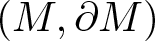 $(M, \partial M)$ is a compact
 $n$-dimensional Riemannian manifold (
 $n \geq 3$) of non-positive curvature such that every geodesic minimizes distance up to the boundary, then
 \begin{equation*}
\mathrm{Vol}(\partial M)^n \geq C(n) \, \mathrm{Vol}(M)^{n-1},
\end{equation*}
where the constant  $C(n)$ is given by
 \begin{equation*}
C(n) = \frac{\alpha(n-1)^{n-1}}{\alpha(n-2)^{n-2} \left( \int_0^{\pi/2} \cos(t)^{n/(n-2)} \sin(t)^{n-2} \, dt \right)^{n-2}},
\end{equation*}
and  $\alpha(n)$ denotes the volume of the unit
 $n$-sphere.
While this inequality is sharp when  $n = 4$, it is only achieved when the manifold is isometric to a flat ball. Therefore, this result does not resolve the isoperimetric problem for the Bergman metric, since the Bergman ball is not flat. The constant
 $C(n)$ is not sharp in the non-flat setting, and hence does not yield equality in the case of the Bergman geometry.
Data availability statement
Data sharing is not applicable to this article since no data sets were generated or analysed.
Funding statement
The author is partially supported by the Ministry of Education, Science and Innovation of Montenegro through the grant Mathematical Analysis, Optimization and Machine Learning.
Competing interests
The author declares that he has no conflict of interest.



