1 Introduction
The problem of applying a sudden rotation to an incompressible fluid from rest, known as spin-up, has been studied in different axisymmetric geometries for several decades. A review for the characterisation of linear and nonlinear instabilities was given in Duck & Foster (Reference Duck and Foster2001) and Park & Hyun (Reference Park and Hyun2008). Among the most frequently studied geometries are the spheres (with or without stratification), for their relevance in atmospheric flows (Greenspan & Howard Reference Greenspan and Howard1963; Clark et al. Reference Clark, Clark, Thomas and Nien-Hon1971), the toroid (Madden & Mullin Reference Madden and Mullin1994) and the circular cylinders without axial flow. This last geometry has been studied either as a combination of two parallel discs set apart at a given distance (see the pioneering work of Wedemeyer (Reference Wedemeyer1964)), or by assuming a small gap, which simulates the conditions of a disc (Krymov Reference Krymov1990).
In this work we analyse what happens to the Hagen–Poiseuille flow with a superimposed rigid rotation (henceforth RHPF) when this rotation is reduced at a given instant of time (spin-down). This particular problem has not been considered in the literature previously. RHPF is a very simple prototype of rotating flows with axial velocity, such as vortices in nature. The main difference between these latter open flows and RHPF is its confinement into the pipe. In addition, RHPF has been thoroughly studied in theoretical and numerical studies, but less experimental data are available, though it is one set-up that is reasonably easy to build and to control accurately.
Most studies compare the flow behaviour and its temporal evolution when a sudden rotation from rest is imposed or when the rotation is stopped suddenly in other different geometries (Bien & Penner Reference Bien and Penner1971; Cui Reference Cui2003; Ogawa & Murakami Reference Ogawa and Murakami2004; Hewitt et al. Reference Hewitt, Hazel, Clarke and Denier2011). The main objective of these works involves studying the regions where the instabilities appear (frequently in the boundary layer close to the rotation-subjected wall, or in the symmetry axis), and computing the time needed to observe an experimental change in the flow structure. Thus, with respect to the dynamic spin-down problem of a fluid confined in a given axisymmetric geometry, the case of a fluid filled torus subjected to spin-down has been analysed theoretically, numerically and experimentally (del Pino et al. Reference del Pino, Hewitt, Clarke, Mullin and Denier2008) as well as the different relations of the toroid’s initial and final rotation velocities, and the case of spin-over (change in swirl direction) has also been studied numerically and theoretically in Hewitt et al. (Reference Hewitt, Hazel, Clarke and Denier2011). The work of Kühnen et al. (Reference Kühnen, Holzner, Hof and Kuhlmann2013) is fundamentally different in that the flow is not driven by the system but by a metal sphere drawn through a toroidal tube instead. In addition, a circular cylinder (without axial flow) has also been analysed for the spin-down case (Weidman Reference Weidman1976; Mathis & Neitzel Reference Mathis and Neitzel1985; Dolzhanskii, Krymov & Manin Reference Dolzhanskii, Krymov and Manin1992), which also simulates the conditions of an infinite cylinder when a large distance separates its circular base and top (Krymov & Manin Reference Krymov and Manin1986). Out of these studies over the circular cylindrical geometry, the closest to the experiment proposed in this paper, can be found in Weidman (Reference Weidman1976) who generalises the criterion given by Wedemeyer (Reference Wedemeyer1964), in the sense that nonlinear instabilities appear more rapidly in the spin-up problem than in the spin-down one. When the cylinder is rotating without axial flow, centrifugal instabilities tend to dominate the spin-down process together with the endwall waves from the top and bottom lids. In this complicated scenario, numerical simulations have provided better understanding to characterise the flow dynamics giving a deeper physical insight into the instability mechanisms which arise in this type of flow (Lopez & Weidman Reference Lopez and Weidman1996). Moreover, in the case of a finite cylinder but with no axial velocity when subjected to sudden spin-down, two facts characterise the flow (Neitzel & Davis Reference Neitzel and Davis1981), namely: the process, which is nonlinear, constitutes an unstable problem due to the appearance of 3D structures even for highly viscous fluids. Furthermore, just to mention some review papers regarding the cylindrical geometry given in this work, the spin-down problem has also been studied in a cylinder with a thermal gradient so as to simulate the processes in the sun (Sakurai Reference Sakurai1969), as well as in the field of oceanography, see, for example Maxworthy & Browand (Reference Maxworthy and Browand1975).
RHPF is a model solution that describes the flow inside a pipe subjected to a pressure gradient, and whose external wall is rotating at a given angular velocity. Two non-dimensional parameters govern the problem: the Reynolds number,
 $Re$
, and the swirl parameter,
 $L$
(see definitions in the next section). The steady solution of this problem can be easily described with the parabolic velocity profile and the solid body rotation for the axial and azimuthal velocities, respectively. The radial velocity profile is null. Although the transition between convective and absolute instabilities for RHPF has already been studied numerically, and various mathematical criteria have been provided for the search of absolutely unstable eigenvalues (Fernandez-Feria & del Pino Reference Fernandez-Feria and del Pino2002; Suslov Reference Suslov2006), its numerical manifestation through direct simulations (Sanmiguel-Rojas & Fernandez-Feria Reference Sanmiguel-Rojas and Fernandez-Feria2005), the description of instability typologies (Heaton Reference Heaton2008) or even the unsuccessful attempt to find finite amplitude solutions (Barnes & Kerswell Reference Barnes and Kerswell2000), few studies have been able to experimentally characterise the onset of absolute instabilities in RHPF (Shrestha et al.
Reference Shrestha, Parras, del Pino, Sanmiguel-Rojas and Fernandez-Feria2013), where the mode (or azimuthal wavenumber)
 $n=-1$
is the most unstable one up to
 $Re\approx 320$
. In fact, the transition from convective to absolute instabilities in RHPF with the presence of an unstable vortex breakdown in the sudden expansion downstream of the rotating pipe using the same experimental set-up described in § 2 is also reported in Miranda-Barea et al. (Reference Miranda-Barea, Martínez-Arias, Parras, Burgos and del Pino2015). Regarding other experimental works, RHPF also exhibits the same behaviour of two parallel discs subjected to different rate rotation: slowly travelling modes are predicted to be the most dangerous within the convectively unstable region (Lingwood & Garrett Reference Lingwood and Garrett2011). Several methodologies have been applied to detect the onset of absolute instabilities in this last geometry (Lingwood Reference Lingwood1996, Reference Lingwood1997a
,Reference Lingwood
b
). In these works the author analyses the stability properties of boundary-layer flows caused by a differential rotation rate between the lower disc and the incompressible fluid in rigid-body rotation above. This configuration results in the known BEK system (Bödewadt, Ekman and von Kármán boundary layers).
Our main region of interest in this manuscript is the inlet region of the rotating pipe where the flow develops until it reaches the conditions of RHPF in the downstream region. The reason why the inlet region is relevant stems from the fact that direct visualisations allow us to detect the transition from convective to absolute instabilities, as we will explain in the following sections. The local, spatial stability analysis using a parallel flow for RHPF is described in Fernandez-Feria & del Pino (Reference Fernandez-Feria and del Pino2002), whose results are used to compare our experimental transitions from convectively to absolutely unstable RHPF in the (
 $Re$
,
 $L$
) plane. In fact, this parallel flow becomes our base flow in the downstream region of the rotating pipe: parabolic profile with solid-body rotation. Though the study of the parallel flow can be understood as a simplification of the real scenario, there are many examples in different geometries where this parallel approximation is still valid to find the most unstable modes versus non-parallel approximations, global stability analyses or the nonlinear convective/absolute instabilities (Delbende & Chomaz Reference Delbende and Chomaz1998b
). On the other hand, we remark on the relevance of four works concerning the analysis of the non-parallel RHPF. Pedley (Reference Pedley1969) analysed the viscous flow instabilities and proposed a criterion to establish the minimum dimensionless length required for RHPF to be fully developed, the entrance length being the greatest between the Reynolds number and the product of Reynolds number by the swirl parameter. This criterion, however, turns out to be rather conservative on account of the numeric and hydrodynamic analyses performed on the non-parallel flow by del Pino, Ortega-Casanova & Fernandez-Feria (Reference del Pino, Ortega-Casanova and Fernandez-Feria2003), who set the length necessary for RHPF to be fully developed between 35 % and 40 % of the length established by Pedley’s criterion. In addition, Imao, Zhang & Yamada (Reference Imao, Zhang and Yamada1989) found that rotation would perturb the flow in the developing region of RHPF, and an overshooting phenomenon in the axial velocity for
 $Re=500$
and
 $L=1.5$
was also studied, numerically and experimentally. Imao et al. (Reference Imao, Itoh, Yamada and Zhang1992) reported experimental evidence of a mode shift from
 $n=-1$
to
 $n=-2$
for
 $Re=500$
, which was also analysed in del Pino et al. (Reference del Pino, Ortega-Casanova and Fernandez-Feria2003). Finally, it is worth mentioning that no global stability analysis for RHPF has been reported yet.
As will be seen in the next sections, this experimental work reports an alternative procedure to provide a simple criterion with which to distinguish the transition from convective to absolute instabilities by direct observation. To the best of the authors’ knowledge, no previous studies have dealt with the spin-down problem taking into account the presence of axial flow in the velocity field, such as is done in the one presented here. Our study focuses mainly in the pipe inlet region as this is the part of the spatial domain where the onset of absolute instability is first observed. Thus, our analysis in the space–time domain represents an alternative experimental methodology to the one given in Shrestha et al. (Reference Shrestha, Parras, del Pino, Sanmiguel-Rojas and Fernandez-Feria2013). This work is organised as follows. First, the experimental set-up along with the dimensionless parameters and measurement techniques are briefly described in § 2. Subsequently, the visualisation results in the downstream and the inlet area of RHPF subjected to a partial stop or a sudden spin-down are accounted for and discussed properly in § 3. In this section, the wave packet fronts observed are characterised by means of spatiotemporal diagrams. Lastly, we remark the main novelty of our work and the conclusions drawn from this experimental study in § 4.
2 Experimental set-up
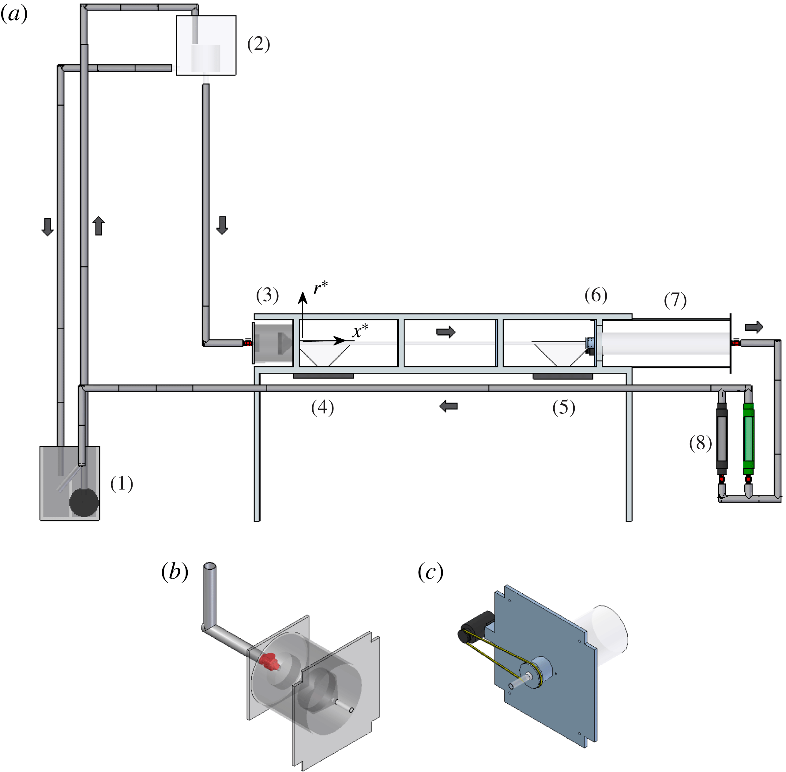
In this section we describe the experimental set-up to help the reader understand the parameters involved in the spin-down process. The arrangement which is shown in figure 1 slightly upgrades that used in Shrestha et al. (Reference Shrestha, Parras, del Pino, Sanmiguel-Rojas and Fernandez-Feria2013) to comply with the requirements of this research. The upgrading consists mainly in the installation of two devices: another flowmeter in parallel to the existing one, which allows greater Reynolds numbers,
 $Re$
, to be reached and one immersed pump which allows both increasing the flow rate and reducing the heating of the working fluid with time, thus ensuring that the kinematic viscosity is kept roughly constant. An aluminium structure holds up the experiment whose different parts are accurately aligned with a digital inclinometer within
 $\pm 0.1^{\circ }$
. The length and the diameter of the horizontal rotating pipe are
 $L_{p}=1960~\text{mm}$
and
 $d=19\pm 0.04~\text{mm}$
, respectively.
Schematic of the experimental set-up (a), and detail of the conditioning chamber (b) and the DC motor (c).

The hydraulic circuit can be described as follows. The water is pumped from a storage deposit (1) to a large head tank (2), which contains another smaller tank inside. When the flow fills up the smaller tank, it starts to fill the head tank which is connected to the storage deposit (1). Due to this design, a pressure drop along the pipe is kept fixed by the constant height between the small tank upstream (high level) and the inlet of the rotating pipe (low level). During each measurement one valve ensures the constant head loss in the hydraulic system. One diffuser, one honeycomb and one converging nozzle (3) set the flow in the inlet region without perturbations. The nozzle is aligned and connected to the rotating pipe with a specially machined aluminium piece which is fitted with one O ring sealing system and a precision bearing. The transparent perspex horizontal rotating pipe allows flow visualisations with two digital video cameras of 1 MP and 25 or 50 f.p.s. (frames per second). The flow visualisations and video recordings are performed in the (
 $r^{\ast }$
,
 $x^{\ast }$
) plane of the rotating pipe inlet region, henceforth referred to upstream (4) and downstream (5) regarding the spatial domain for
 $d\leqslant x^{\ast }\leqslant 15d$
and
 $82d\leqslant x^{\ast }\leqslant 90d$
, respectively. The procedure to highlight the flow patterns consists of projecting the light beam from the halogen lamps (4 or 5) through a thin rectangular hole practised in a dark paper. This results in white light sheets which strike the pipe vertically. To improve the visualisation and recording of the flow patterns, the fluid is seeded with 2 % of Kalliroscope© AQ1000, which is a suspension between 1 % and 2 % of reflective flakes with a typical size of
 $30~{\rm\mu}\text{m}\times 6~{\rm\mu}\text{m}\times 0.07~{\rm\mu}\text{m}$
, see Kalliroscope© Corporation for details (or see Savas Reference Savas1985). This additive has a relatively large reflective optical index
 $n_{op}=1.85$
, and its density is equal to
 ${\it\rho}=1.62~\text{g}~\text{cm}^{-3}$
.
The angular rotation is driven with a DC motor (6) which is connected to the pipe with a transmission belt in the downstream region of the rotating pipe. The motor is closed-loop controlled, and the velocity of the motor is known by means of an encoder. This feedback control is quite good to keep an error within 0.5 % between the desired and the current angular velocities. The water temperature is measured before and after each test to take into account the changes in the kinematic viscosity, the temperature variation being lower than
 $0.1\,^{\circ }\text{C}$
. Likewise, to avoid flow disturbances downstream, a sudden expansion (7) is connected to the end of the rotating pipe. Finally, one or two flowmeters (8) can be used depending on the flow rate employed before the flow moves to the initial storage tank (1). At least a set of three different tests were carried out for each experimental point.
The coordinate system employed comprises the cylindrical coordinates (
 $r^{\ast }$
,
 $x^{\ast }$
,
 ${\it\theta}$
), the superscript asterisk denoting dimensional variables, and setting the origin (
 $x^{\ast }=0$
) in the joint area between the convergent nozzle which is found in the conditioning chamber upstream of the rotating pipe, and the rotation subjected pipe. We include in this work the observation and characterisation of the various states occurring in the pipe inlet region of a circular cylinder when a non-parallel axial flow is developed after being subjected to rigid-body rotation. The final state depends on the combination of two parameters: the Reynolds number (
 $Re$
) and the swirl parameter (
 $L$
). The Reynolds number is defined with the expression
 $Re=U\cdot d/{\it\nu}=4\cdot Q/({\rm\pi}\cdot d\cdot {\it\nu})$
, where
 $U$
is the mean velocity,
 ${\it\nu}$
is the kinematic viscosity and
 $Q$
is the flow rate. The dimensionless parameter
 $L$
is defined as the inverse of Rossby number for a flow in an uniform section circular pipe, by
 $L={\it\Omega}\cdot d/(4\cdot U)$
,
 ${\it\Omega}$
being the angular velocity. The experiments were carried out with
 $Re$
ranging between 100 and 600. Therefore, the study of laminar pipe flow is performed for low-to-moderate
 $Re$
, i.e.
 $Re\leqslant 600$
. This upper limit is based on the criterion of the maximum pipe length reported by Pedley (Reference Pedley1969) and its numerically worked-out correction given by del Pino et al. (Reference del Pino, Ortega-Casanova and Fernandez-Feria2003). Thus, it can be stated that we have a fully developed RHPF downstream of the pipe, as we will demonstrate in the following section. Obviously, no turbulence has been observed for this range of
 $Re$
and the values of
 $L$
tested.
3 Results and discussion
3.1 Flow visualisations
3.1.1 Downstream region
First, we give some explanations regarding the spatial stability analysis in RHPF. The reader must note that the determination of local absolute instabilities by adopting the Briggs–Bers criterion (Briggs Reference Briggs1964; Bers Reference Bers1975) requires the so-called parallel-flow approximation (see figure 9 below where we present the neutral curves in solid and dashed lines given by Fernandez-Feria & del Pino Reference Fernandez-Feria and del Pino2002). Actually, we set a pair of values
 $Re$
,
 $L_{0}$
in the (
 $Re$
,
 $L$
)-plane to reach a given initial state before applying the spin-down. If RHPF is stable (S.), it will reach a steady base flow solution. However, if this flow has convective (C.I.) or absolute instabilities (A.I.), it will reach a limit cycle around the base flow solution, since a periodic unstable spiral (
 $n=-1$
or
 $n=-2$
) appears in the downstream region. In other words, we use the expression limit cycle to define the situation where RHPF becomes time-dependent because travelling waves appear in the downstream region while applying a critical rotation to the pipe flow
 $L_{0}$
greater than
 $L_{c}$
or
 $L_{a}$
, thus becoming convectively or absolutely unstable, respectively (see again figure 9). Shrestha et al. (Reference Shrestha, Parras, del Pino, Sanmiguel-Rojas and Fernandez-Feria2013) have reported that flow visualisations in the inlet region (
 $2d\leqslant x^{\ast }\leqslant 11d$
) have already provided a method to distinguish between stable and unstable solutions, and between C.I. and A.I., showing that the values of the measured frequencies and wavelengths in the downstream region are in good agreement with those obtained by a spatial, linear stability analysis with the parallel-flow approximation. This analysis works well when constant values of
 $Re$
and
 $L_{0}$
were tested experimentally, though it was impossible to determine the transition between C.I. and A.I. by direct observation in the downstream region.
In this new study we present a novel experimental methodology based on the spin-down process through direct observations in the upstream region (see supplementary material available online at http://dx.doi.org/10.1017/jfm.2016.122). However, we must ensure that the base flow is RHPF in the downstream region even after applying the spin-down, that is to say, when the flow changes from the pair
 $Re$
,
 $L_{0}$
to
 $Re$
,
 $L_{f}$
. To that end, we set a pair
 $Re$
,
 $L_{0}$
inside the absolutely unstable region and we will reduce the swirl parameter up to a certain value
 $L_{f}$
. The spatial and temporal axes are non-dimensionalised with the characteristic length
 $L_{c}=d/2=9.5~\text{mm}$
and characteristic time
 $t_{c}=L_{c}/W_{0}$
,
 $W_{0}=2U$
being the maximum axial velocity which depends on the Reynolds number tested. The non-dimensional variables
 $r=r^{\ast }/L_{c}$
,
 $x=x^{\ast }/L_{c}$
and
 ${\it\tau}=t/t_{c}$
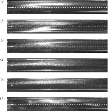
stem from these characteristic magnitudes defined above. Figure 2 shows snapshots in a (
 $r$
,
 $x$
) plane at different dimensionless times in the spin-down process, (a–f) corresponding to
 ${\it\tau}=0$
–50 with time steps equal to 10, for a constant Reynolds number,
 $Re=250$
. As the reader will note in all of the snapshots the flow moves from left to right (positive
 $x$
indicates positive flow rate, see figure 2).
Flow visualisations for
 $Re=250$
and
 $L_{0}=2$
and
 $L_{f}=1.0$
, at certain times
 ${\it\tau}=0$
(a), 10 (b), 20 (c), 30 (d), 40 (e) and 50 (f) in the spatial domain
 $164\leqslant x\leqslant 179$
.

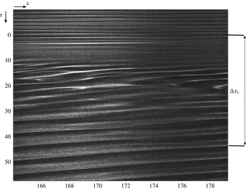
Figure 3 represents the spatiotemporal diagram which results from the flow visualisations presented in figure 2 in a cut of the symmetry axis (
 $r=0$
) in the downstream region. The flow starts with an initial and final swirl parameters
 $L_{0}=2$
and
 $L_{f}=1$
, respectively. Patterns appear periodically up to
 ${\it\tau}=0$
, when the spin-down has been applied, and they reappear at
 ${\it\tau}={\rm\Delta}{\it\tau}_{1}$
, being
 ${\rm\Delta}{\it\tau}_{1}\approx 45$
, approximately. Obviously, the slope in the spatiotemporal diagram changes from
 $L_{0}$
to
 $L_{f}$
as a consequence of the variation in the swirl parameter, and because the flow reaches a new oscillatory state too. Recall that the flow is convectively unstable in figure 3 for
 $L=L_{f}$
.
Spatiotemporal diagram for
 $Re=250$
and
 $L_{0}=2$
and
 $L_{f}=1.0$
.

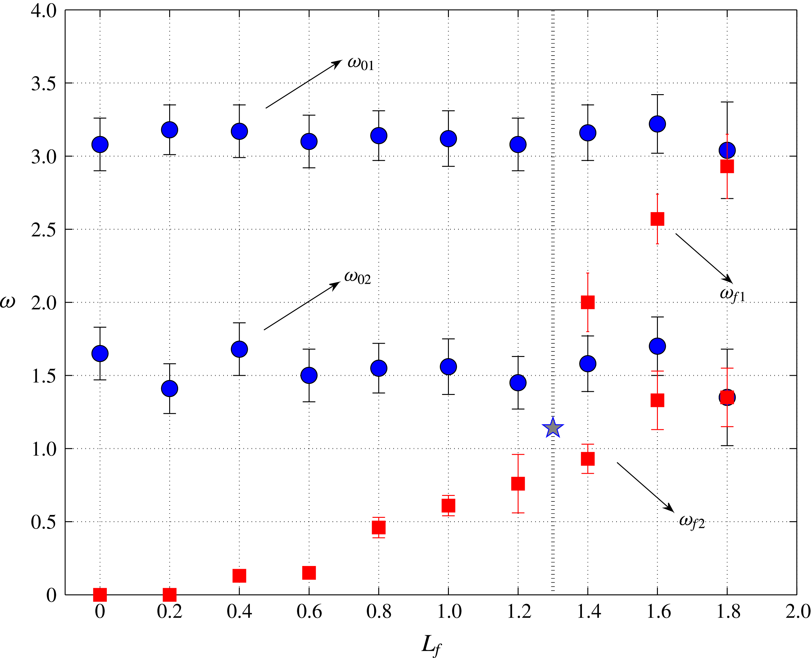
Dimensionless frequencies for
 $Re=250$
and
 $L_{0}=2$
(
 ${\it\omega}_{0}$
, blue circles) with different
 $L_{f}$
(
 ${\it\omega}_{f}$
, red squares). Only the highest frequencies of
 ${\it\omega}$
correspond to the predominant modes resulting from 1D FFT (marked with subscript 1). The star indicates the theoretical frequency for the transition from convectively to absolutely unstable flow given in Fernandez-Feria & del Pino (Reference Fernandez-Feria and del Pino2002).

On the other hand, we are able to compute dimensionless real frequencies,
 ${\it\omega}$
, from the spatiotemporal diagram presented in figure 3, being
 ${\it\omega}=\hat{{\it\omega}}R/W_{0}$
, where
 $\hat{{\it\omega}}$
is the dimensional frequency obtained by using one-dimensional (1D) fast Fourier transform (FFT). The results are shown in figure 4 for different reductions of the rotation speed, while keeping constant the Reynolds number,
 $Re=250$
, and the initial value of the swirl parameter,
 $L_{0}=2$
. We define
 ${\it\omega}_{0}$
(blue circles) as the frequencies which correspond to the initial swirl parameter
 $L_{0}$
(negative
 ${\it\tau}$
in figure 3), while
 ${\it\omega}_{f}$
(red squares) belong to the periodic patterns after applying the spin-down process (
 ${\it\tau}$
greater than
 ${\rm\Delta}{\it\tau}_{1}$
in figure 3). One explores a set of experiments under the same initial conditions (
 $Re$
,
 $L_{0}$
), so the frequencies at which the flow is oscillating are roughly constant,
 ${\it\omega}_{01}\approx 3.15$
, thus confirming the reliability of the results. The subscript 1 in
 ${\it\omega}_{01}$
and
 ${\it\omega}_{f1}$
defines the predominant frequencies at
 $L_{0}$
and
 $L_{f}$
, respectively. One must note that the experimental points
 ${\it\omega}_{01}$
and
 ${\it\omega}_{f1}$
tend to be equal as the reduction jump, defined as
 ${\rm\Delta}L=L_{0}-L_{f}$
, approaches zero (
 ${\rm\Delta}L\rightarrow 0$
), confirming again a good experimental procedure. In addition, the critical swirl parameter
 $L_{f}=L_{a}=1.3$
corresponds to the threshold between convective and absolute instabilities using the local, spatial stability analysis with a parallel-flow approximation for azimuthal wavenumber
 $n=-1$
(see again figure 9 below Fernandez-Feria & del Pino Reference Fernandez-Feria and del Pino2002). This stability analysis also provides the frequency for the onset of absolute instabilities. Therefore, the pair
 $(L_{a},{\it\omega}_{a})=(1.3,1.14)$
is also depicted in figure 4 with one star symbol. The theoretical prediction
 ${\it\omega}_{a}$
is in excellent agreement with the trend of the experimental points
 ${\it\omega}_{f1}$
. This fact confirms that the flow is RHPF in the downstream region after applying the spin-down process. In addition, other experimental peaks of (secondary) frequencies also appear while performing 1D FFT, and they are shown with subscript 2 (
 ${\it\omega}_{02}$
and
 ${\it\omega}_{f2}$
) in figure 4. It is worth mentioning that the values of
 ${\it\omega}_{02}$
are half the predominant frequencies
 ${\it\omega}_{02}={\it\omega}_{01}/2\approx 1.57$
. We observe the same behaviour after applying the spin-down process from
 $L_{0}$
to
 $L_{f}$
, so
 ${\it\omega}_{f2}\approx {\it\omega}_{f1}/2$
. Curiously, only peaks of (secondary) frequencies
 ${\it\omega}_{f2}$
are present for swirl parameters
 $L_{f}$
greater than
 $L_{a}$
.
Three main features stem from the analysis of figure 4: first, the experimental procedure is reliable because only small errors appear in the computation of the frequencies (
 ${\it\omega}_{0}$
,
 ${\it\omega}_{f}$
) and, second, the linear theory with a parallel approximation accounts quite well for the RHPF stability after applying the spin-down process. As mentioned in the introduction, this last characteristic is important as it was also highlighted in other flows such as two-dimensional wakes, see Delbende & Chomaz (Reference Delbende and Chomaz1998b
). Thirdly, we do believe that the appearance of second real frequency peaks, with a magnitude half the predominant ones, can only be related to the presence of other mode with
 $n=-2$
that interacts with the predominant one
 $n=-1$
within the absolutely unstable region. This mode shift from
 $n=-1$
to
 $n=-2$
will be presented in the last section.
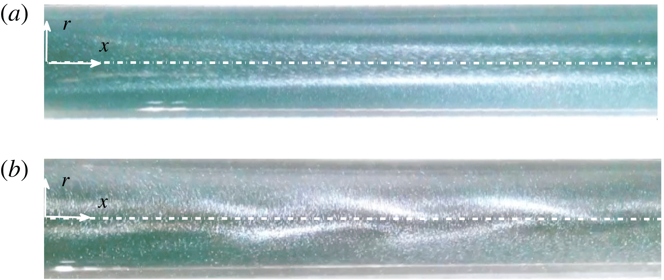
Images of convectively (a) and absolutely unstable flows (b) for
 $Re=500$
and
 $L=0.8$
and 1.5, respectively. The spatial domain corresponds to
 $2\leqslant x\leqslant 14$
.

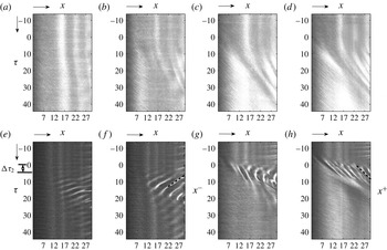
Spatiotemporal diagrams for
 $Re=250$
and originally unstable states: convectively
 $L_{0}=1$
(a–d) and absolutely
 $L_{0}=2$
(e–f). The reduction of the angular velocity is of the size: 30 % (a–e), 50 % (b–f), 80 % (c–g) and 100 % (d–h). We depict the time
 ${\rm\Delta}{\it\tau}_{2}$
and the negative and positive slopes (
 $x^{-}$
and
 $x^{+}$
, respectively) with dashed black lines.

3.1.2 Upstream region
In this section we describe the different states that were found experimentally in RHPF in the pipe inlet next to the conditioning chamber. The onset of absolute instabilities was experimentally characterised in Shrestha et al. (Reference Shrestha, Parras, del Pino, Sanmiguel-Rojas and Fernandez-Feria2013) by means of the appearance of a spiral structure in the pipe inlet region, such as observed in figure 5 in the spatial domain
 $2\leqslant x\leqslant 14$
. These snapshots for
 $Re=500$
allow a precise distinction between convectively (a) and absolutely (b) unstable flows for
 $L=0.8$
and
 $L=1.5$
, respectively, in RHPF following the criterion given in Shrestha et al. (Reference Shrestha, Parras, del Pino, Sanmiguel-Rojas and Fernandez-Feria2013): the flow upstream of the pipe is considered stable, so the propagation of travelling waves downstream with negative group velocity interact with the flow in the inlet region forming the characteristic spiral pattern. However, direct visualisations of the absolutely unstable flow and the subsequent appearance of spirals in the pipe inlet region are far from being sharp just in the transition area (see figure 2d in Shrestha et al. (Reference Shrestha, Parras, del Pino, Sanmiguel-Rojas and Fernandez-Feria2013)). For this reason, it was necessary to generate a spatiotemporal diagram in the inlet region so that the spiral structures there would become much clearer. This is shown in figure 6 for
 $Re=250$
and
 $L_{0}=1$
(a–d) or
 $L_{0}=2$
(e–h) in the spatial domain
 $2\leqslant x\leqslant 30$
. We now pay special attention on the values
 ${\it\tau}$
lower than zero which correspond to a constant initial value of the swirl parameter
 $L_{0}$
, while the features regarding the application of the spin-down process (positive
 ${\it\tau}$
) will be discussed below. Thereby, the onset of absolute instabilities was experimentally observed as a sequence of spirals in the pipe inlet region which, consequently, show up as different colour bands parallel to the temporal axis of the spatiotemporal diagram, the spatial domain being the symmetry axis,
 $r=0$
(see also figure 4c in Shrestha et al. (Reference Shrestha, Parras, del Pino, Sanmiguel-Rojas and Fernandez-Feria2013)). Thus, these parallel bands in figure 6(e–h) for negative values of
 ${\it\tau}$
reveal the presence of spiral patterns which correspond to the onset of absolute instabilities so the pair
 $L_{0}=2$
and
 $Re=250$
belongs to the absolutely unstable region. The same patterns are observed in these figures as a consequence of the same initial conditions. However, with swirl parameters close to the end of the convectively unstable flow, see figure 6(a–d) for
 $L_{0}=1$
when the critical value of the swirl parameter is
 $L_{a}\approx 1.3$
, we still observe a sequence of bands which might be taken as absolutely unstable cases. A plausible cause may be that the transition from convectively to absolutely unstable flows is gradual in RHPF in the sense that flow patterns do not change abruptly but rather slightly with increasing
 $Re$
or
 $L_{0}$
. In addition, the problem of visualisation-based direct observations in the transition area becomes harder and harder as
 $Re$
increases, so the spiral structure shown in figure 5(b) is not too clear. This shortcoming justifies this experimental visualisation-based alternative by spinning down the rotating pipe or spinning it down to rest has been developed in order to establish the transition from convective to absolute instabilities experimentally. Another inconvenience derived from direct visualisation is that there is no possibility to distinguish between
 $n=-1$
and
 $n=-2$
modes in a (
 $r,x$
) plane. We will be back to figure 6 after explaining in detail the video given as supplementary material.
For the characterisation of the flow states in the pipe inlet, namely, convectively and absolutely unstable flows, we resort to a new experimental method so as to distinguish between them. This new experimental procedure is based on the nature of the hydrodynamic instabilities (Huerre & Monkewitz Reference Huerre and Monkewitz1998): whereas the convective instabilities tend to disturb the flow downstream, the absolute ones affect all of the spatial domain, even the pipe inlet region where the flow is developing, and is supposedly stable. This is due to the fact that convectively unstable travelling waves tend to propagate more intensely downstream, i.e. the group velocity is positive (
 $c_{g}>0$
). However, absolute instabilities tend to destabilise the flow in the region where RHPF is developing, i.e. in the pipe inlet, thereby one could observe the change from the initial typical conical structure (figure 5
a) into the already-mentioned spiral structure (figure 5
b). The reason for this change in the flow structure is that the absolute-instabilities-produced wave packets tend to propagate more intensely both downstream and upstream, i.e. the group velocity is negative (
 $c_{g}<0$
). The transition takes place, in mathematical form, for the null group velocity and this is the experimental critical point when it comes to determining where the transition takes place.
On grounds of what has been previously explained, for the experimental analysis we set a given
 $Re$
and
 $L=L_{0}$
to establish the RHPF. Once the initial state has been established in the pipe, we reduce the angular velocity, its new value ranging from 1 % (infinitesimal variation) to 100 % (spin-down to rest or sudden stop). In fact, for a given reduction of the angular velocity, which depends on
 $Re$
and
 $L_{0}$
, we have been able to clearly identify the transition from convective to absolute instability. Further in the text we discuss the computation of the relative value of the angular velocity reduction required for an instability to take place but, first, it is essential to describe the temporal evolution of RHPF in the pipe inlet. The experimental methodology is based on the variation of the swirl parameter from an initial state, which can be convective or absolute, to a final state with one randomly-chosen swirl parameter,
 $L_{f}$
, lower than that initially adopted,
 $L_{0}$
. By following this experimental procedure, the video attached to this manuscript illustrates one temporal sequence in the (
 $r$
,
 $x$
) plane for
 $Re=250$
and initial convective state (
 $L_{0}=0.8$
) and absolute state (
 $L_{0}=2$
) with a 50 % reduction of the rotation speed for different times. The sequence of images show the temporal evolution of the perturbation-produced wave packet fronts in the pipe inlet region. Therefore, the criterion adopted to distinguish whether or not the wave packet fronts propagate towards to the inlet is the drastic variation observed in the perturbations which were originally convective or absolute. In convectively unstable flows, perturbations do not alter the structure of the inlet whatever reduction of the rotation speed is applied during the spin-down process, so the wave packet fronts only move downstream in the video for
 $L_{0}=0.8$
, confirming the nature of the perturbations given in Huerre & Monkewitz (Reference Huerre and Monkewitz1998). In addition, it is also clear in the video how the instability grows upstream towards to the pipe inlet region when
 $L_{0}=2$
. This change results as a consequence of the wave packet propagation upstream, thus confirming again the absolute nature of the instability. In some cases, the wave packet fronts disappear in the inlet region of the pipe where the convergent nozzle is placed, as its opacity does not lend itself to visualisation. As far as we know, this is the first experimental evidence of a temporal evolution of absolute instabilities in RHPF. Recall again that the flow moves to the right in the video, and in figures 5 and 6, as indicated above, providing the reference point for the distinction between upstream and downstream.
The advantage of the experimental method presented here with respect to that given in Shrestha et al. (Reference Shrestha, Parras, del Pino, Sanmiguel-Rojas and Fernandez-Feria2013) is that no spatiotemporal diagram is needed as one can distinguish whether the flow is convectively or absolutely unstable simply with a direct observation. However, the next step is to quantify the experimental measurements performed in order to validate the success of the experimental procedure reported in this paper.
As we indicated above, we repeat the same procedure to build spatiotemporal diagrams given in figure 3, but for the upstream region instead of the downstream region. Figure 6 displays the results for different reductions in the swirl parameter for
 $Re=250$
: convectively unstable states (a–d) and absolutely unstable states (e–h). The spatiotemporal diagrams in figures (a–d) correspond to an initial swirl parameter
 $L_{0}=1$
and reductions of 30 % (a), 50 % (b), 80 % (c) and 100 % (d), whereas the ones in figures (e–h) correspond to an initial swirl parameter
 $L_{0}=2$
, and the same values of the reduction given above. We will pay our attention on positive values of
 ${\it\tau}$
. The origin of the time axis corresponds to the beginning of the partial/total reduction of the swirl parameter within the timing errors of the mechanical response of the system.
In this work we go one step further studying the temporal evolution while varying the value of the swirl parameter as it may become an efficient experimental method to detect the onset of absolute instabilities. This process can be described as follows. While the transient process takes place as a result of a partial or total reduction of the swirl parameter applied to initial convectively unstable flows, a temporal evolution of the wave packet is observed, its transient front moving with positive velocity. However, when the reduction is applied to initial absolutely unstable flows, the wave packet front appears moving counterflow-wise (with negative velocity). Actually, we can confirm the presence of a wave packet travelling upstream until it is blocked by the inlet in our confined flow, see figure 6(e–f) for
 ${\it\tau}$
approximately greater than 5. The experimental results presented in figure 6(e–h) are also similar to the data reported by Chomaz (Reference Chomaz2003) in his numerical study for wakes in open flows while studying the fully nonlinear dynamics of this type of flows.
The experimental evidence presented in figure 6 depends on the level of reduction of the angular velocity which is also function of
 $Re$
and
 $L_{0}$
,
 ${\rm\Delta}L/L(\%)=f(Re,L_{0})$
. Thus, the characteristic velocity of the wave packet front (
 $c^{+/-}$
) can be computed with the quotient
 $x^{+/-}/t$
which corresponds to light bands in figure 6. One can observe that positive and negative upper scripts denote light bands from figure 6 with slopes greater or lower than zero. In other words, rays with positive slope show patterns flowing with positive flow rate (from left to right).
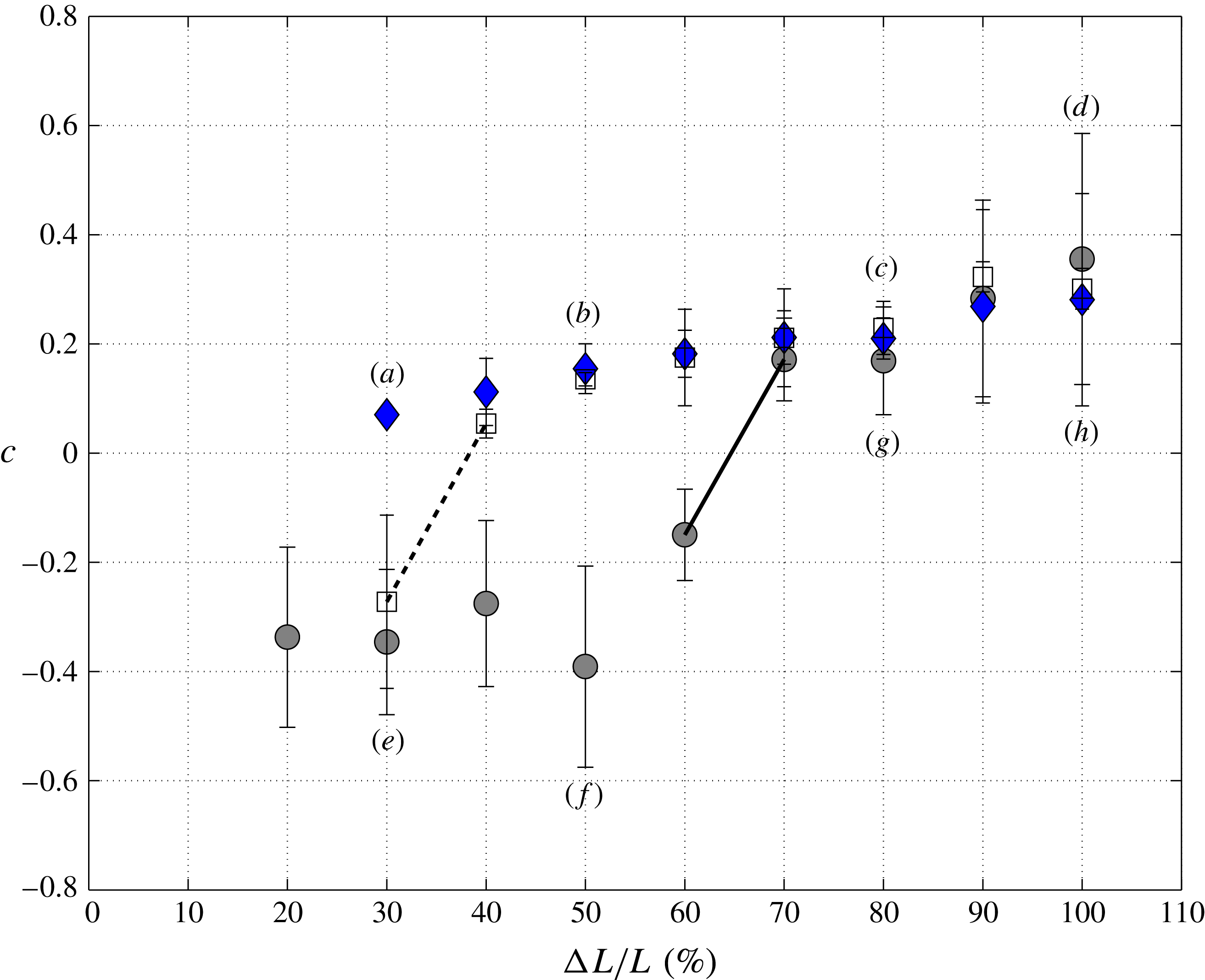
Evolution of the velocity of the wave packet front in terms of the reduction of the swirl velocity for cases which are originally convectively unstable (blue diamonds,
 $L_{0}=1$
) and absolutely unstable (grey circles,
 $L_{0}=2$
) together with the theoretical threshold from convective to absolute instabilities (white squares,
 $L_{0}=1.3$
). The labels (a–h) correspond to figure 6.

To quantify the velocity
 $c^{+/-}$
, different reference points have been chosen (between three or five rays, depending on the spatiotemporal diagram) and their mean values and standard deviation have been computed. In figure 7 the values of the velocity
 $c$
are plotted in terms of the decreasing rate of swirl for a constant Reynolds number,
 $Re=250$
, and for the same cases of swirl velocity reduction shown in figure 6, to which some extra cases have been added. It is observed that for the initial convectively unstable cases, depicted with diamonds (
 $L_{0}=1$
), the velocities are always positive (
 $c=c^{+}$
). However, in the initial absolutely unstable cases, which correspond to circles (
 $L_{0}=2$
), there exists a critical value of the swirl reduction, from which the flow visualisations start to give negative values (
 $c^{-}$
). In fact, the critical reduction of the swirl parameter, for which
 $c=0$
, is found to be near 65 %. There are values in the
 $x$
axis which are not plotted in figure 7, as for example those where the reduction is less than 20 % (convectively unstable,
 $L_{0}=1$
) or less than 10 % (absolutely unstable,
 $L_{0}=2$
). This lack of information stems from the fact that no characteristic
 $c^{+}$
or
 $c^{-}$
have been observed in the spatiotemporal diagram through direct flow visualisations. In other words, the flow does not present variations which can be identified visually for (infinitesimal) low reductions in the angular velocity, and then there is no experimental evidence of wave front movements. Therefore, in these particular cases, it is observed that the critical value
 ${\rm\Delta}L/L(\%)$
decreases almost to the region which cannot be observed experimentally. For values
 $L_{0}$
lower than the critical swirl parameter,
 $L_{0}=L_{a}=1.3$
, all the velocity values computed are positive (
 $c=c^{+}$
, i.e.
 $L_{0}=1$
), confirming the experimental methodology used in this work. We also depict one solid and one dashed line in figure 7 to highlight the jump from
 $c^{-}$
to
 $c^{+}$
for
 $L_{0}=2$
and 1.3, respectively.
It remains an open question why spin-down produces a change in the flow behaviour allowing us to detect by direct observations the change from convective or absolute instabilities. We do believe that a plausible answer could be related to the linear impulse response of the RHPF. On the one hand, a small a variation in the rotation causes the inlet flow to have a negative ray (see, e.g., figure 6
e or f), while on the other hand a significant reduction of the swirl parameter makes the flow behave as it were convective; compare, e.g., figure 6(d) and (h). In our view the aspect ratio in the reduction of the rotation speed to visualise the change in the flow during the spin-down process (from negative to positive as we increase the reduction ratio of the swirl parameter) is conditioned by the initial values of the two parameters that govern this problem:
 $Re$
and
 $L_{0}$
. The further this pair of values inside the absolutely unstable region is from the neutral curve of the convectively unstable region in the (
 $L,Re$
) plane, the greater the amount of reduction of the swirl parameter is required. The flow behaves in a different manner starting with (
 $L_{0},Re$
) from the A.I. region and finishing in the A.I. region with (
 $L_{f}$
,
 $Re$
) or starting in the A.I. region and finishing on the C.I. region. If we apply a linear response while decreasing the swirl parameter, we need at least a 20 % reduction to observe the effect of the spin-down through flow visualisations. This amount of reduction of the angular velocity should be lower in case of a numerical study. Thus, once we force a reduction of the angular velocity, this jump is convected from the wall side to the axis in the radial direction. To attain the new final state the flow needs a certain period of time, so at the axis of the pipe it remains absolutely unstable with the same characteristics as the starting swirl number
 $L_{0}$
. We do know that one vortex responds to any perturbation by generating waves to readapt the flow. In this case, the waves travelling upwards through the axis of the pipe are quicker than those generated in the wall through a sudden reduction of the angular velocity. Depending on how strong the reduction rate is, those waves propagating from the wall in radial direction are stronger or weaker than the absolute instabilities. These unstable waves travel upwards finding a stable flow which reduces their energy in the entrance of the pipe. That is the reason why the flow needs a given strength of the reduction rate for the perturbation to be clearly distinguishable through flow visualisations in the entrance of the rotating pipe, and this value cannot be predicted theoretically by easy means: only the competition between absolute instabilities in RHPF and centrifugal modes due to the spin-down process could clarify this point. Finally, it is also worth mentioning that a small reduction of the swirl parameter during the spin-down process could be seen as an impulsive response of RHPF for large time. This is also discussed using the Batchelor vortex in Delbende & Chomaz (Reference Delbende and Chomaz1998a
), where they describe the numerical procedure to determine the change from convective to absolute instabilities by using the complex streamwise wavenumber and the complex frequency observed along each spatiotemporal ray
 $v_{g}=x/t$
for large time. Unfortunately, there is no possibility to compute the resulting growth rate given in Delbende & Chomaz (Reference Delbende and Chomaz1998a
) through flow visualisations.
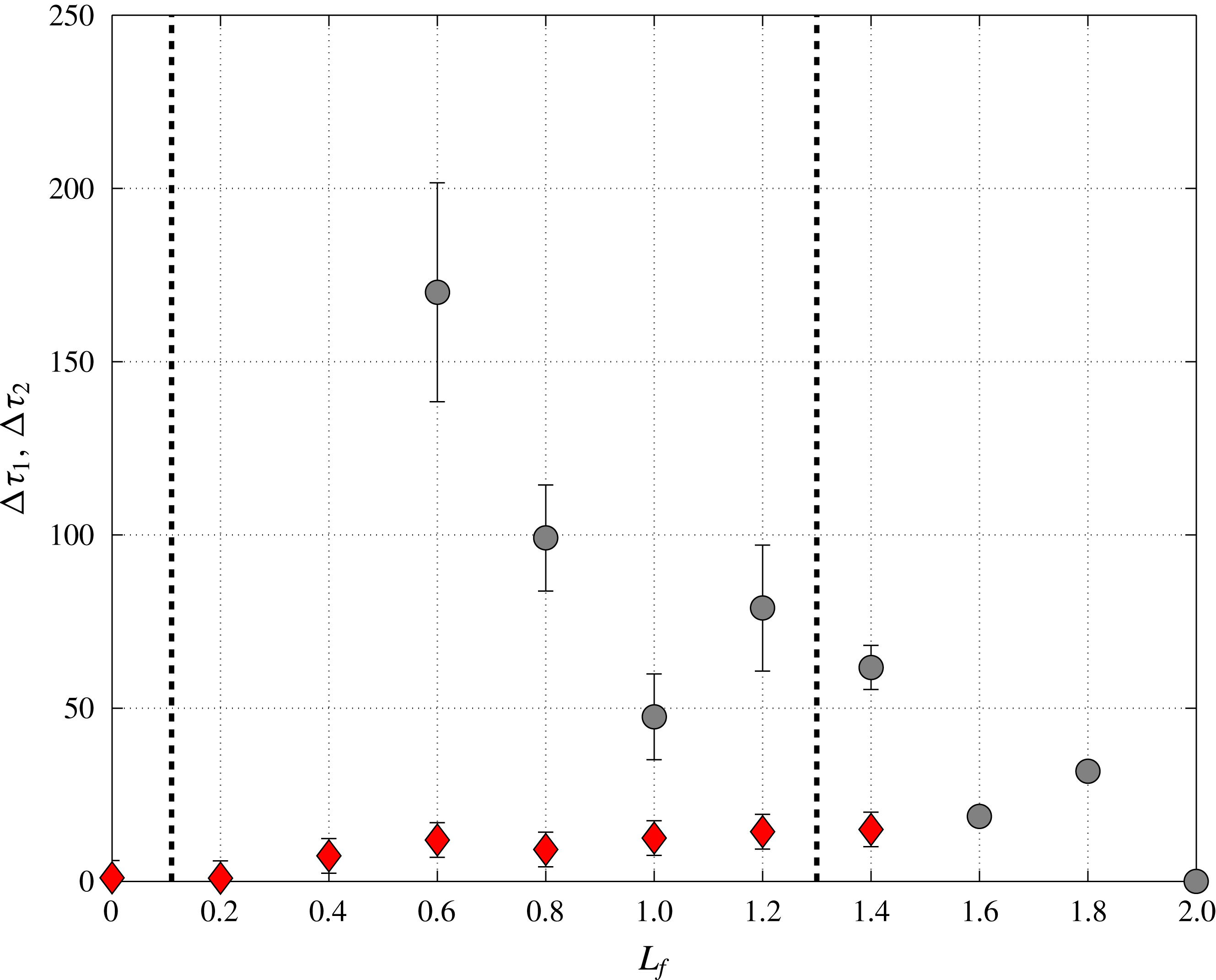
Dimensionless time
 ${\rm\Delta}{\it\tau}_{1}$
for the spin-down process in the downstream region (grey circles, see figure 3) and
 ${\rm\Delta}{\it\tau}_{2}$
corresponding to the upstream region (red diamonds, see figure 6) for different values of the final values of the swirl parameter
 $L_{f}$
, the initial state being
 $Re=250$
and
 $L_{0}=2$
. In dashed lines, it is depicted the critical values
 $L_{c}=0.11$
and
 $L_{a}=1.3$
given in Fernandez-Feria & del Pino (Reference Fernandez-Feria and del Pino2002).

3.2 Time evolution of the flow
We are dealing with a complex problem where the base flow varies both in space and time, and it reaches a fully developed steady state only at long distances and large times. Once we have confirmed the experimental procedure to detect the onset of absolute instabilities in the inlet region of the pipe, we focus on the spin-down process in terms of the time required to attain the final state. This keypoint plays an important role to discard the interaction of the transient flow produced in the downstream region with that generated in the upstream region. That is to say, there is no influence on the flow formation in the downstream region when it is varying from
 $L_{0}$
to
 $L_{f}$
and the wave fronts are propagating upstream. To that end, we analyse again figures 3 and 6 for the case
 $Re=250$
and
 $L_{0}=2$
. We compute two different times when we apply a spin-down process up to constant value
 $L_{f}$
,
 ${\rm\Delta}{\it\tau}_{1}$
(grey circles) and
 ${\rm\Delta}{\it\tau}_{2}$
(red diamonds). Both times are based in spatiotemporal diagrams. We define
 ${\rm\Delta}{\it\tau}_{1}$
as the time to reach a new state in the downstream region or the time required by the flow to form again periodic patterns (transient period shown in figure 2), while
 ${\rm\Delta}{\it\tau}_{2}$
, which has the origin at
 ${\it\tau}=0$
, is the time required to observe the onset of perturbations (or rays) to compute
 $c^{+}$
or
 $c^{-}$
in the upstream region (see figure 6). The results of applying these definitions to different cases are shown in figure 8 in which we also depict the data regarding the theoretical swirl parameter at which transition from stable to convectively unstable flow,
 $L_{c}=0.11$
, together with the transition between convectively and absolutely unstable flows,
 $L_{a}=1.3$
, using a parallel approximation (see Fernandez-Feria & del Pino Reference Fernandez-Feria and del Pino2002). We can confirm that there are two different time scales which correspond to the time evolution of the RHPF from
 $L_{0}$
to
 $L_{f}$
and the wave front propagation up to the inlet region, both being unrelated, so the spin-down process in the downstream region of the rotating pipe has a weak influence on the wave propagation in the upstream region because there is no connection between them. The flow converges to a new steady state in the downstream region for times larger than appearance of instabilities in the upstream region of the rotating pipe. As shown in figure 8,
 ${\rm\Delta}{\it\tau}_{1}$
can be estimated on a theoretical basis for the Ekman-layer formation time because it is found to be proportional to the inverse of
 ${\rm\Delta}L$
when
 $L_{f}$
is close to
 $L_{0}$
(see Weidman Reference Weidman1976). In addition, we can consider that time response of the base flow is slow enough for a classical stability analysis to remain valid, confirming that the parallel and local analysis developed in Fernandez-Feria & del Pino (Reference Fernandez-Feria and del Pino2002) is still applicable in the downstream region. This stems from the fact that as
 $L_{f}$
approaches
 $L_{c}$
(remember that
 $L_{c}$
is marking the critical value from stable to convectively unstable flow),
 ${\rm\Delta}{\it\tau}_{1}$
tends to infinity because the stable base flow would not present further perturbations downstream. To conclude, the time
 ${\rm\Delta}{\it\tau}_{2}$
to attain the new state for the final pair (
 $Re$
,
 $L_{f}$
) is much lower than the time
 ${\rm\Delta}{\it\tau}_{1}$
, so the typical timescale in terms of the wave propagation in the region upstream of the rotating pipe is found to be two orders of magnitude lower than the typical timescale of the base flow variation in the downstream region when RHPF varies from
 $L_{0}$
to
 $L_{f}$
. Therefore, RHPF is mainly controlled by the modes contained in the initial state for the pair (
 $Re$
,
 $L_{0}$
) during the spin-down process.
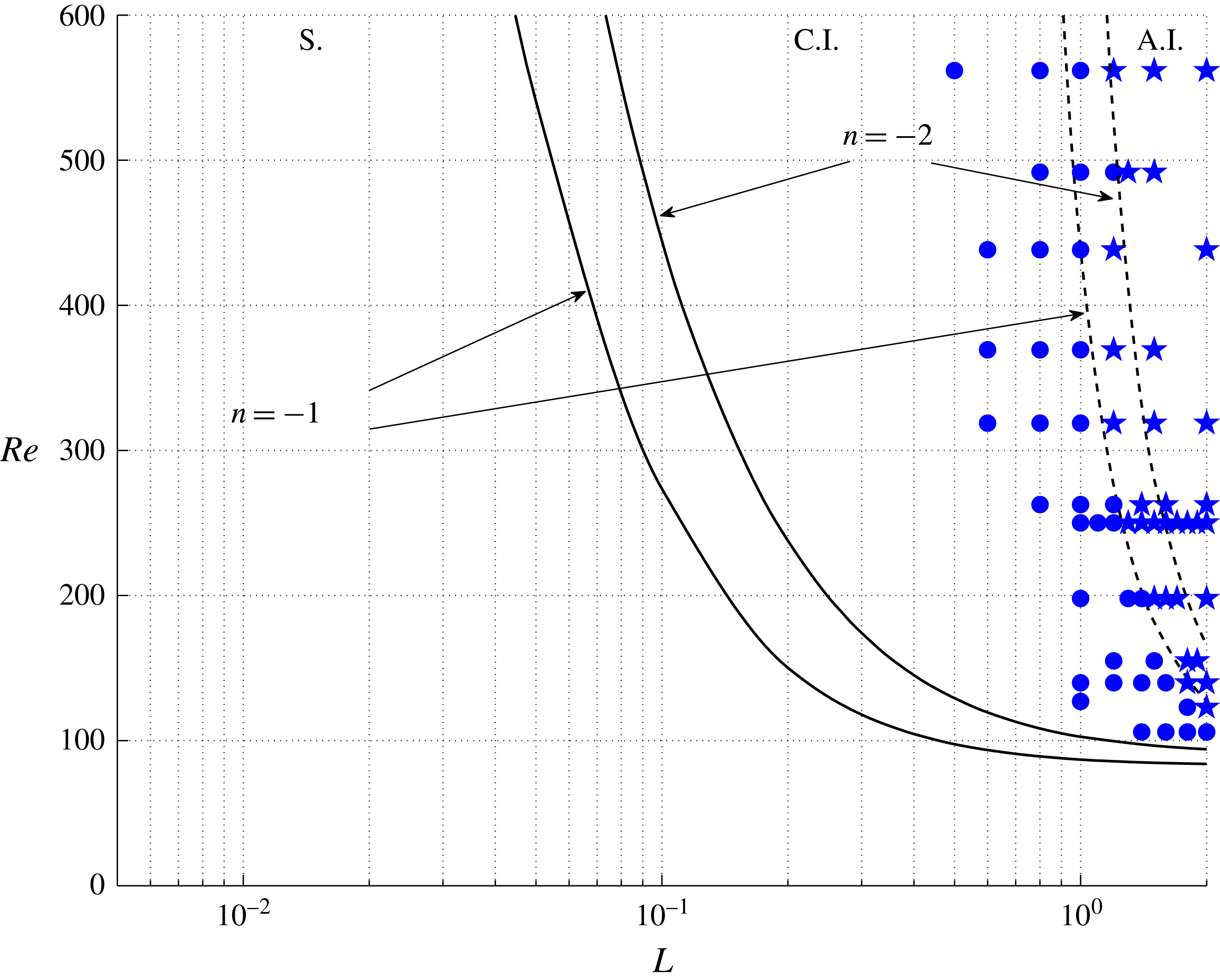
Plot of the experimental states in the (
 $Re$
–
 $L$
)-plane: stable (S.), convective (C.I., circles) and absolute instabilities (A.I., stars). In the same graphic the theoretical curves obtained by Fernandez-Feria & del Pino (Reference Fernandez-Feria and del Pino2002) are introduced for azimuthal wavenumbers
 $n=-1$
and
 $n=-2$
, one (solid line) depicting the transition from the stable flow (S.) to the convectively unstable flow and the other (dashed line) depicting the transition from the latter to the absolutely unstable flow.

3.3 Results in the
 $Re$
–
$L$
plane


All the experimental states characterised with the (experimental) methodology presented in this paper are summarised in figure 9. In this plot it is observed that the experimentally obtained results close to the transition between C.I. and A.I. are in good agreement with the theoretical data reported in Fernandez-Feria & del Pino (Reference Fernandez-Feria and del Pino2002) for the most unstable mode (dashed line for the onset of and A.I.). Therefore, in view of the results shown in figure 9, there exist regions where the theoretical curves coincide with the experimental data for
 $n=-1$
or
 $n=-2$
. The same experimental scenario was reported in Imao et al. (Reference Imao, Itoh, Yamada and Zhang1992). Numerically del Pino et al. (Reference del Pino, Ortega-Casanova and Fernandez-Feria2003) also performed a non-parallel stability analysis in the developing region of the pipe, where both unstable modes were found simultaneously for
 $Re=500$
and swirl parameters ranging from
 $L_{0}=0.5$
to 1.5. In our case, there is a smooth transition from
 $n=-1$
to
 $n=-2$
from
 $Re=300$
to 500. Finally, it must be also remarked that the analysis of the region where the flow is stable (S.) has been discarded as it is beyond the scope of this work, whose main objective is to provide a simple criterion to detect the onset of absolute instabilities.
4 Conclusions
A new experimental characterisation of RHPF has been performed in the inlet region of a circular pipe between convectively and absolutely unstable flows when a spin-down or a spin-down to rest are produced. The onset of absolute instabilities was characterised by observing different structures in the developing region, i.e. a change from the initial typical conical structure to the spiral structure, with wave packet fronts appearing in this area, or otherwise by a spatiotemporal diagram, see Shrestha et al. (Reference Shrestha, Parras, del Pino, Sanmiguel-Rojas and Fernandez-Feria2013). However, a new experimental methodology is proposed here to distinguish between the two unstable experimental states through direct visualisation of the flow. This allows us to distinguish easily the flow state by varying the swirl parameter from a given value to the partial or sudden stop, visualising the effect of wave packets propagation in the inlet spatial domain. It has been checked that in initial convectively unstable flows, the wave packet fronts provoked by the instability never perturb the flow in the inlet region of the rotating pipe, whereas in the threshold of absolute instability, the front of the transient wave packet propagates to the pipe inlet region, and succeeds in destabilising it. The reason for this is that the wave packets produced by absolute instabilities tend to propagate more intensely both downstream and upstream due to the temporal response of the RHPF during the spin-down process. Through the knowledge of the transition from the convective instabilities to the absolute ones, and its divergence with respect to the theoretical curve given in Fernandez-Feria & del Pino (Reference Fernandez-Feria and del Pino2002) for
 $n=-1$
, we have been able to add a new characteristic to RHPF: the mode shift to
 $n=-2$
which is set around
 $Re=300{-}500$
, finding an excellent agreement with the experimental observations given in Imao et al. (Reference Imao, Itoh, Yamada and Zhang1992) and the corresponding non-parallel stability analysis reported in del Pino et al. (Reference del Pino, Ortega-Casanova and Fernandez-Feria2003). Finally, the authors highlight that it is still an open question whether the spin-down is also a reliable tool for the onset of absolute instabilities in other flow fields subjected to rotation. In addition, further research could be done regarding the other problem that stems from that presented in this experimental work: it should be interesting to explore how RHPF behaves as the swirl parameter is constant and the Reynolds number is partially or totally reduced.
Acknowledgements
The authors are very grateful for the comments of the anonymous referees that have improved the original version of the manuscript. The authors would like to thank S. Pinazo for his technical support and drawings of the experimental set-up. They would also like to acknowledge the fruitful proofreading kindly accomplished by their colleague I. Davison, a man from Coventry. This research has been partially funded by Proyecto de Excelencia de la Junta de Andalucía, grant number P11-TEP-7776.
Supplementary movie
Supplementary movie is available at http://dx.doi.org/10.1017/jfm.2016.122.