NOMENCLATURE
-
 ${\sigma _{\rm{x}}}$
-
stress in warp direction
-
${\sigma _y}$
-
stress in weft direction
-
${\varepsilon _x}$
-
strain in warp direction
-
${\varepsilon _y}$
-
strain in weft direction
-
${E_x}$
-
elastic modulus in warp direction
-
${E_y}$
-
elastic modulus in weft direction
-
${\upsilon _{yx}}$
-
Poisson’s ratio in warp direction
-
${\upsilon _{xy}}$
-
Poisson’s ratio in warp direction
-
${x_1},...,{x_N}$
-
coordinates of nodes
-
${y_1},...,{y_N}$
-
interpolated values at data locations
-
$\Re $
-
set of real numbers
-
${\alpha _j}$
-
expansion coefficients
-
$g(x)$
-
set of any radial basis functions
-
$F(x)$
-
RBF interpolant
- AE
-
average error
- ME
-
maximum error
- RMSE
-
root-mean-square error
- N
-
number of samples
-
$Y$
-
real values
- c
-
average value
-
$H$
-
transfer matrix


1.0 INTRODUCTION
The world’s first airship dates back to 1784, when hydrogen was used to provide buoyancy and the propulsion propeller was hand powered(Reference Stockbridge, Ceruti and Marzocca1). The development of airships entered its heyday in the 1920s. Nevertheless, the research into and operation of airships stagnated during 1930–1937 due to several fires and crashes as well as the rise of conventional aircraft. In recent years, the airship has attracted renewed attention due to the benefits of helium use and the rapid development of new energy sources, materials science and control techniques. A non-rigid airship is a cost-effective alternative to satellites in Earth orbit for sightseeing, aerial photography, communications and weapon transport. Many countries have plans to develop airships, resulting in a significant increase in expected usage.(Reference Alam and Pant2-Reference Wang4) For a non-rigid airship, the envelope, which is located outside the ballonet, is an essential structure that creates the aircraft’s external shape as well as providing balance.(Reference Stockbridge, Ceruti and Marzocca5,Reference Mayer6) Plain-weave fabrics are the materials most commonly used on non-rigid airships because they are light, flexible and durable, characteristics that are critical as the material bears almost all the weight of the envelope.(Reference Bin-Tai, Li-Ying, Pei-Gang and Xiang-bao7) It is thus critical when designing the envelope to study the stress–strain characteristics of the material. To describe its mechanical properties, the envelope material is regarded as elastic, nonlinear elastic(Reference Ambroziak8), viscoelastic(Reference Argyris, St. Doltsinis and da Silva9) or viscoplastic(Reference Klosowski, Zagubien and Woznica10) in many analysis models. The choice of the model is conditioned by the type of coated fabrics, but is always disputable. In 1997, based on the micromechanical behaviour of a representative unit cell, Nayfed proposed a non-linear constitutive model for plain-weave fabrics(Reference Nayfeh and Kress11). In 2007, Nedjar presented a fully three-dimensional constitutive model for anisotropic viscoelasticity that is suitable for a macroscopic description of fibre-reinforced composites under finite strains(Reference Nedjar12). In 2017, Meng obtained several invariant values reflecting the characteristics of the envelope material according to invariant theory(Reference Meng and Lv13). In 1992, Severn(Reference Maheri and Severn14) compared a number of experimental results with mass added to a flexible structure using classical added mass theory for rigid-body vibration. It was found that classical added mass theory is only applicable to bodies with a single degree of freedom.
A non-rigid airship with different stress ratios in the warp and weft directions exhibits a complex force condition. To date, biaxial tensile testing has been the preferred method to study the mechanical properties of plain-weave fabrics.(Reference Lili and Liye15) The MSAJ standard(16) is the only existing and widely accepted standard for biaxial testing of woven fabrics. The American Standard ASCE–1852 (1996)(17) also recommends the MSAJ standard. All the work described below is based on the MSAJ standard. In 2012, Li introduced the method of the MSAJ standard to calculate the mechanical behaviour of Ferrari1302 laminate fabrics(Reference Li18), finding that the membrane exhibited complex mechanical properties depending on the geometric size, sample, test conditions, test system, load ratio, load history and different data analysis methods applied. In 2015, Ambroziak tested the mechanical properties of Précontraint 1202S coated fabric using biaxial tensile testing at different load ratios(Reference Ambroziak19), successfully identifying the material parameters based on biaxial and uniaxial tensile tests. In 2017, Chen studied the detailed mechanical behaviour and determined the proper elastic parameters for URETEK3216LV plain-weave fabrics in specific stress states(Reference Chen, Chen and Wang20). The results showed typical stress–strain curves consisting of three distinct regions during loading: a crimp region, a nonlinear transition region and a yarn extension region, being consistent with those of the constitutive yarns.
The MSAJ standard approximates the stress–strain relationship of plain-weave fabrics using a plane orthotropic model, and the mechanical performance parameters are obtained by employing the least-squares method. Because of the complicated structural relationship in plain-weave fabrics, the stress–strain relationship under biaxial tension becomes highly nonlinear(Reference Peirce21-Reference Tan and Barnes23). However, the MSAJ standard is not suitable for describing such nonlinear relationships, only enabling a simple assessment of the overall mechanical properties of the material test piece. Compared with the MSAJ standard, approximate methods can reflect the stress–strain relationship more accurately and directly. Bridgens used spline functions to define the response surfaces of coated woven fabrics(Reference Bridgens and Gosling24). Chen used elastic parameter response surfaces to reveal the mechanic behaviour of URETEK3216LV plain-weave fabrics(Reference Ambroziak19). For nonlinear models, a curved surface enables a better representation of the experimental material characteristics(Reference Galliot and Luchsinger25).
UN-5100 is a plain-weave composite with reasonable consistency, low helium permeability, thin density and appropriate strength. As a common skin material for stratospheric airships, it is necessary to study its material characteristics experimentally. Currently, research on the properties of materials used in stratospheric airships is primarily based on biaxial tensile testing, but the results of that analysis method are not accurate; For example, the elastic constant measured according to the MSAJ standard will describe the nonlinear characteristics using a linear method. The primary purpose of this study is thus to select a test and analysis method that can describe the material properties more accurately to meet the practical engineering requirements of the application. In this work, the stress–strain relationship was tested in different stress conditions. Using DIC technology and Isight software, stress–strain curves were corrected and more accurate experimental curves were obtained. By comparing the slope of the curves, the MSAJ standard, and the RBF model, various conclusions on the mechanical properties of the flexible airship material are obtained and may play an essential role in the design of such envelopes.
2.0 THEORY
2.1 Elastic parameters based on least-squares method
In the MSAJ standard, the mechanical performance parameters are obtained based on the least-squares method. As the thickness of plain-weave materials is minimal, it is generally considered that their mechanical properties are orthotropic elastic and thus that the corresponding stress–strain relationship can be approximated using an orthotropic plane model:
 \begin{equation}\left\{ {\begin{array}{*{20}{c}}{{\varepsilon _x}}\\[3pt]{{\varepsilon _y}}\end{array}} \right\} = \left[ {\begin{array}{*{20}{c}}{\frac{1}{{{E_x}}}}&{ - \frac{{{\nu _{xy}}}}{{{E_y}}}}\\[3pt]{ - \frac{{{\nu _{{\rm{yx}}}}}}{{{E_x}}}}&{\frac{1}{{{E_y}}}}\end{array}} \right]\left\{ {\begin{array}{*{20}{c}}{{\sigma _x}}\\[3pt]{{\sigma _y}}\end{array}} \right\}\end{equation}
where
 $\varepsilon $
is the strain,
 $\sigma $
is the stress, E is the elastic modulus,
 $\upsilon $
is the Poisson’s ratio, and the subscripts x and y denote the warp and weft directions, respectively. The above formula can be simplified to
 \begin{equation}{E_{{\rm{11}}}} = \frac{1}{{{E_x}}},\ {E_{{\rm{22}}}} = \frac{1}{{{E_y}}},\,{E_{{\rm{12}}}} = - \frac{{{\upsilon _{xy}}}}{{{E_y}}},\ {E_{{\rm{21}}}} = - \frac{{{\upsilon _{yx}}}}{{{E_x}}}\end{equation}
For orthotropic elastic materials, the Poisson’s ratio and elastic modulus are constrained by the Maxwell relationship:
 \begin{equation}\frac{{{\upsilon _{xy}}}}{{{E_y}}} = \frac{{{\upsilon _{yx}}}}{{{E_x}}}\end{equation}
From Equations (2) and (3), it can be determined that
 ${E_{{\rm{21}}}} = {E_{{\rm{12}}}}$
. Under different stress ratio loads, the sum of the squares of the strain difference can be obtained as
 \begin{equation}{\rm{S = }}\sum {\left[ {{{({E_{{\rm{11}}}}{\sigma _{xi}} + {E_{12}}{\sigma _{yi}} - {\varepsilon _{xi}})}^2}} \right]} + \sum {\left[ {{{({E_{{\rm{12}}}}{\sigma _{xi}} + {E_{22}}{\sigma _{yi}} - {\varepsilon _{yi}})}^2}} \right]} \end{equation}
where i represents the experimental data obtained at the i-th stress ratio. Using the principle of the minimum sum of squares of strain residuals, the derivative of the unknown variables is equal to 0:
 \begin{equation}\frac{{\partial {\rm{S}}}}{{\partial {E_{{\rm{11}}}}}} = \frac{{\partial {\rm{S}}}}{{\partial {E_{{\rm{12}}}}}} = \frac{{\partial {\rm{S}}}}{{\partial {E_{22}}}} = 0\end{equation}
Combining Equations (4) and (5) yields
 \begin{equation}\left[ {\begin{array}{c@{\quad}c@{\quad}c}{\sum {\sigma _{xi}^2} }&{\sum {{\sigma _{xi}}{\sigma _{yi}}} }&0\\[3pt]{\sum {{\sigma _{xi}}{\sigma _{yi}}} }&{\sum {\!\left( {\sigma _{xi}^2 + \sigma _{yi}^2} \right)} }&{\sum {{\sigma _{xi}}{\sigma _{yi}}} }\\[4pt]0&{\sum {{\sigma _{xi}}{\sigma _{yi}}} }&{\sum {\sigma _{yi}^2} }\end{array}} \right]\left\{ {\begin{array}{*{20}{c}}{{E_{11}}}\\[3pt]{{E_{12}}}\\[3pt]{{E_{22}}}\end{array}} \right\} = \left\{ {\begin{array}{c}{\sum {{\sigma _{xi}}{\varepsilon _{xi}}} }\\[3pt]{\sum {({\sigma _{yi}}{\varepsilon _{xi}} + {\sigma _{xi}}{\varepsilon _{yi}}} )}\\[3pt]{\sum {{\sigma _{yi}}{\varepsilon _{yi}}} }\end{array}} \right\}\end{equation}
From Equations (2) and (6), the Poisson’s ratio (
 ${\upsilon _{yx}},{\upsilon _{xy}}$
) and elastic modulus (
 ${E_x},{E_y}$
) can be obtained.
According to this theoretical background, the method for calculating the elastic modulus and Poisson’s ratio can now be established in principle, by applying the following fitting methods. There are some limitations when using the least-squares method in response surface modelling, as the algorithm cannot deal with some nonlinear effects. When the relationship between the independent and dependent variables of the prototype to be modelled is not simple linear or quasi-linear, the prediction performance will be significantly reduced.
2.2 RBF model in Isight
The RBF model in Isight follows the method of Hardy(Reference Hardy26) described by Kansa(Reference Kansa27). Let
 ${x_1},...,{x_N} \in \Omega \subset {\Re ^N}$
be a given set of nodes. Let
 ${g_i}(x) = g(\| {x - {x_j}} \|) \in \Re $
,
 $j = 1,2,...,N$
be a set of any radial basis functions. Here,
 $\| {x - {x_j}} \|$
is the Euclidian distance given by
 ${\left( {x - {x_j}} \right)^T}\left( {x - {x_j}} \right)$
. We are given the interpolation values
 ${y_1},...,{y_N} \subset \Re $
at data locations
 ${x_1},...,{x_N} \in \Omega \subset {\Re ^N}$
.
By solving the system of N + 1 linear equations with N + 1 unknown expansion coefficients
 ${\alpha _j}$
:
 \begin{equation}\sum\limits_{j = 1}^N {{\alpha _j}} {g_j}({x_i}) + {\alpha _{N + 1}} = {y_i},\ \ i = 1,...,N\end{equation}
 \begin{equation}\ \sum\limits_{j = 1}^N {{\alpha _j}} = 0\end{equation}
the RBF interpolant is obtained as
 \begin{equation}F(x) = \sum\limits_{j = 1}^N {{\alpha _j}} {g_j}(x) + {\alpha _{N + 1}}\end{equation}
Introducing the notation:
 $p = \left[ {\begin{array}{*{20}{c}}1\\ \vdots \\1\end{array}} \right] \in {\Re ^N}$
,
 $G = \left( {\begin{array}{*{20}{c}}{{g_1}({x_1})}& \cdots &{{g_N}({x_1})}\\ \vdots & \ddots & \vdots \\{{g_N}({x_1})}& \cdots &{{g_N}({x_N})}\end{array}} \right) \in {\Re ^{N \times N}}$
,
 $H = \left[ {\begin{array}{*{20}{c}}G&p\\{{p^T}}&0\end{array}} \right] \in {\Re ^{(N + 1) \times (N + 1)}}$
,
 $\alpha = {({\alpha _1},...,{\alpha _{N + 1}})^T}$
and
 $y = {({y_1},...,{y_N},0)^T} \in {\Re ^{N \times N}}$
. The system of Equations (7) and (8) can be rewritten in matrix form as
 \begin{equation}H\alpha = y\end{equation}
The interpolation expansion coefficients are then given by
 \begin{equation}\alpha = {H^{ - 1}}y\end{equation}
One can then easily find the derivatives of the interpolant at any node
 ${x_i}$
,
 $i = 1,2,...,N$
.
Isight uses a function with variable power splines and a radial basis that can be tuned to approximate a large number of other functions:
 \begin{equation}g(x) = {\| {x - {x_j}} \|^c}\end{equation}
where c is a shape function variable between 0.2 and 3.
3.0 EXPERIMENTAL PROGRAM
3.1 Experimental materials and preparation
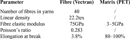
The UN-5100 used in this study is a type of plain-weave material previously applied in stratospheric airships. The properties of the warp and weft yarns are the same, and it exhibits low air permeability, strong environmental corrosion resistance, high strength and low density. The fibre used in UN-5100 is Vectran, with polyethene terephthalate (PET) for the thermal bonding and helium barrier layers. The material properties of UN-5100 are presented in Table 1.
Parameters of UN-5100 material

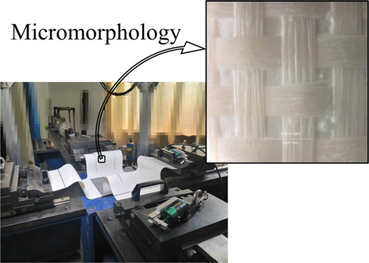
According to the manufacturer, the uniaxial tensile strength of UN-5100 is 568/540cm/N (at room temperature) in the warp and weft direction, respectively. Its micromorphology and material properties are shown in Fig. 1.
The micromorphology of UN-5100 material.

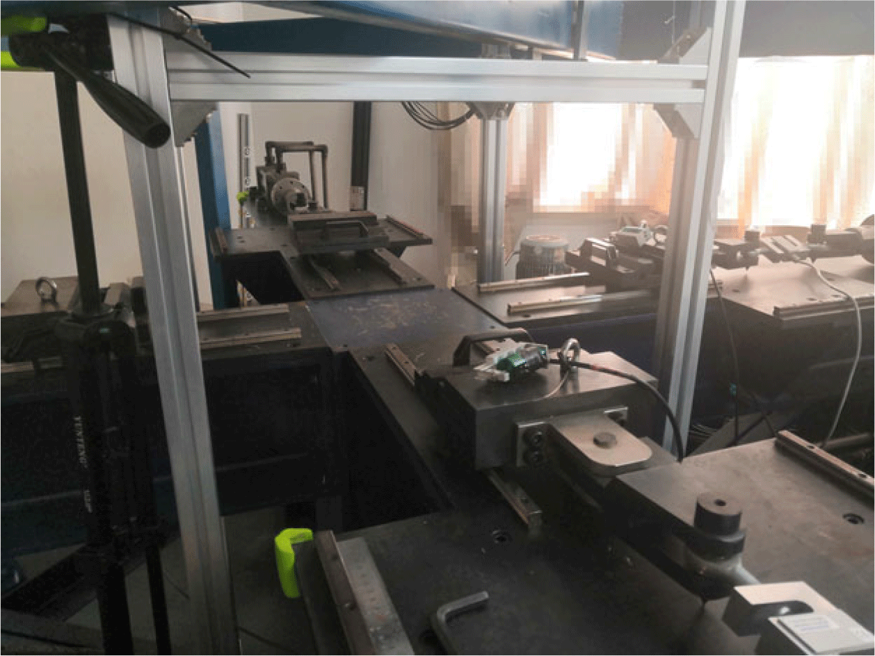
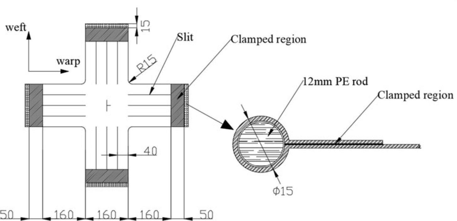
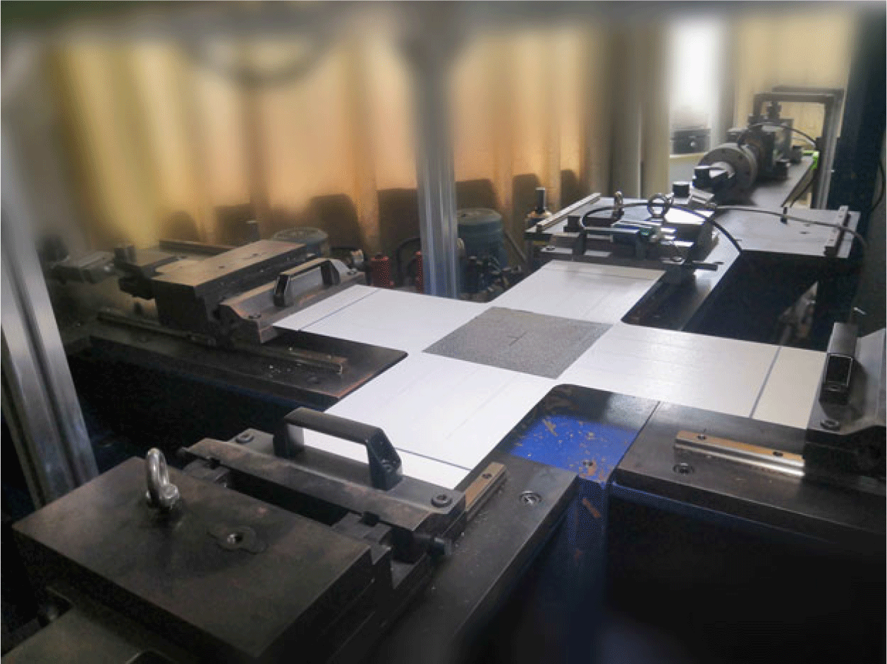
Biaxial testing was carried out using a self-developed biaxial tensile testing machine (SJTU-I), shown in Fig. 2. The strain measurement range of the test machine is 0–20%, the standard tensile rate of the fixture is 2–4mm/min, and the real-time control is 1–5μs. On the power device, a precise servohydraulic cylinder is used, with precise flow control being realised using a proportional valve and overflow valve. Moreover, using force sensor closed-loop feedback and a proportional–integral–differential (PID) controller, a load with any proportion in two directions can be obtained. The biaxial specimen parameters according to standard ISO1421-1998 are shown in Fig. 3. PE rods were fixed on the extension arms to apply longitudinal and latitudinal stress to the sample. The stress through the specimen was kept as moderate as possible under the action of the slits. Digital image correlation (DIC) technology is used instead of extensometers to obtain higher-precision strains. DIC is a non-contact full-field measurement method, which offers the advantages of a wide strain range, high precision, simple equipment, low requirement regarding the test environment and smooth operation.
SJTU-I biaxial tensile testing machine.

Biaxial specimen (units: millimetres)

3.2 Test procedure
The experiment was carried out at humidity of 60
 $ \pm $
4.0% and temperature of 23
 $ \pm $
2.0°C. To remove residual strains and avoid high initial levels of creep, pre-stress of 200N was applied in the warp and weft direction, respectively, as shown in Fig. 4. This method also offers the advantage of preventing the specimen from being slack in its initial state. The application of this initial strain means that the tested stress–strain curves will not pass through the origin, which is compensated for in the data analysis.
The initial state of the specimen.

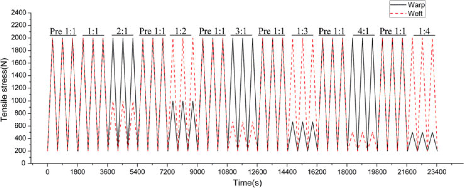
The stress loading was carried out according to the following test protocol, as shown in Fig. 5.
In envelope materials under typical stress states, the ratio between the warp and weft stress ranges from 1:2 to 2:1, but may reach 4:1 in some areas. Therefore, seven loading ratios of 1:1, 1:2, 2:1, 1:3, 3:1, 1:4 and 4:1 were selected. In Fig. 5, ‘Pre 1:1’ indicates the pre-loading with a stress ratio of 1:1. In contrast to the pre-stress, the purpose of this pre-loading is to avoid the influence of residual deformation before and after loading at different stress ratios.
The test protocol.

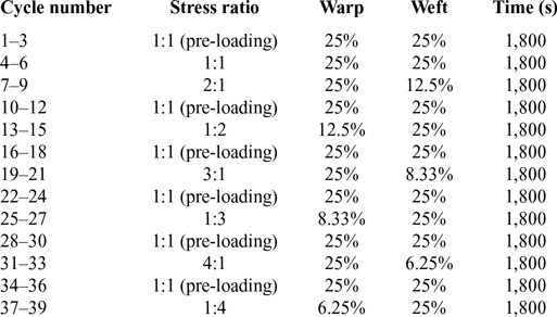
According to the results of uniaxial testing, 20–25% of the uniaxial strength is generally accepted as the maximum value in biaxial tensile loading tests. According to the code for the structural design of airships (FAA-P-8110-2(28)), the safety factor for strength is ≥4. Considering the difference between the warp and weft strength values, the lowest value of 1/4 is broadly employed. Table 2 presents the ratio of the maximum test loading value to the ultimate strength in the warp and weft directions.
Loading history of biaxial tensile test

4.0 RESULTS AND ANALYSIS
4.1 Cyclic stress–strain behaviour of UN-5100 material
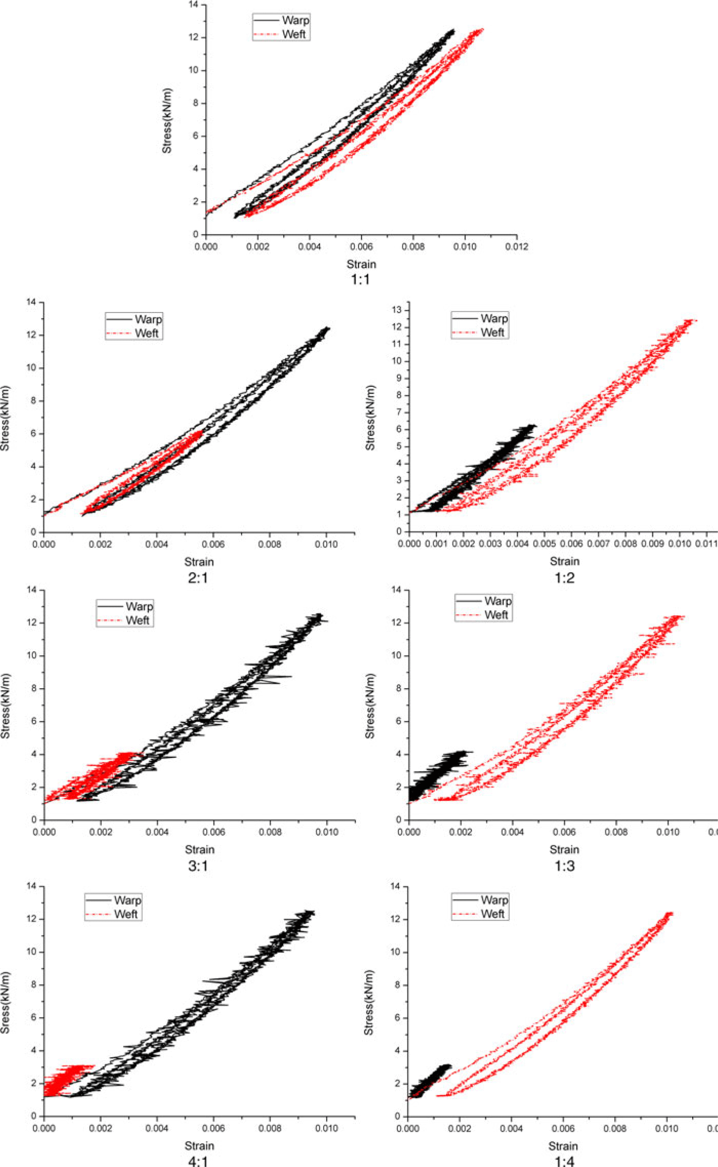
Seven loading ratios were tested, each being cycled three times. Figure 6 shows the stress–strain curves of the specimen at different ratios, where the strain is the machine’s measurement for the entire specimen. From this figure, it is seen that the stress–strain curve stabilises in the third cycle. Accordingly, subsequent analysis was based on the results for the third cycle.
Cyclic curves of stress and strain at each stress ratio.

4.2 Analysis
Taking advantage of DIC technology, the strain at the centre of the specimen can be accurately deduced from the third cycle at the different ratios. Note that there is an initial stress in the specimen at the beginning of the experiment, resulting in an error between the obtained and actual stress–strain curves. It is assumed that, when the stress is 0, the strain is also 0. Consequently, using the approximate model in Isight software(Reference Yu-yang and Xin29), the polynomial curves can be constructed to fit the experimental results. Finally, the error value at different ratios can be obtained and corrected.
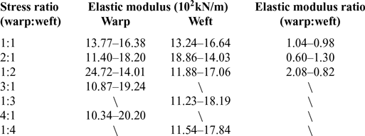
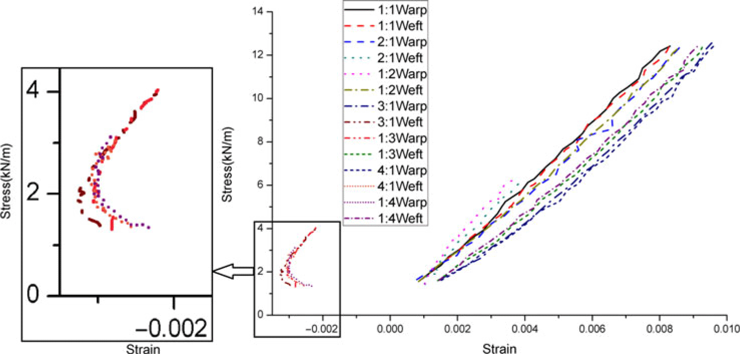
As seen from Fig. 7, the strain is negative in the direction of lower stress when applying the higher stress ratios (3:1, 1:3, 4:1 and 1:4). This indicates that, when under a condition of high stress ratio, the specimen will exhibit necking in the low-stress direction. Also, when the specimen is in the necking stage, the stress–strain curve remains relatively constant. This demonstrates that, in the case of biaxial stress, once at a high stress ratio that causes necking in one direction, the stress–strain relationship in the other direction remains the same. Given that the stress–strain curve is nonlinear, the theory of plane anisotropy cannot be applied, because the plane anisotropy model describes a linear relationship. It can be determined from Equation (1) that the stress–strain relationship of a plain-weave material is linear. In engineering, in order to characterise the mechanical properties of materials, the concepts of elastic properties and the Poisson’s ratio are employed. Therefore, the principle of plane anisotropy is generally applied to describe the stress–strain relationship of skin materials. However, the structural layer of the envelope material is composed of warp and weft yarns, and the interference between them complicates the material’s stress–strain characteristics, resulting in a local nonlinear phenomenon, as seen in Fig. 7. Failure to consider such phenomena could affect the structural safety of the airship. The slope of the stress–strain curve can be used to obtain the elastic modulus in each direction, which is presented in Table 3.
Ranges and ratios of the elastic modulus under different stress ratios

The final stress–strain curves.

According to the results presented in Table 1, when under biaxial tension, the elastic modulus of the stratospheric airship envelope material is greatly affected by the stress and the stress ratio. Under a high stress ratio, the stress–strain curve of the material changes significantly and exhibits visible nonlinear characteristics. Therefore, the elastic modulus and Poisson’s ratio cannot be used to describe the stress–strain relationship of the envelope material in some regions with high stress ratio.
4.3 Results based on MSAJ standard
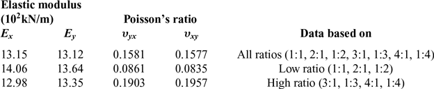
When the elastic modulus is introduced into the plane anisotropic model to describe the stress–strain relationship of a material, the stress–strain model is simplified to a linear model. As a result, the elastic modulus and other parameters must be changed regularly to capture the nonlinear relationship of the actual stress and strain, and sometimes the elastic modulus cannot explain the stress–strain relationship of a material (e.g. when the slope angle of the stress–strain curve is π/2). Additionally, the elastic modulus method cannot yield the elastic parameters for a single stress ratio, but only two or more stress ratios. Following the least-squares method described above, the elastic modulus and Poisson’s ratio of the specimen were calculated, and the results are presented in Table 4. The elastic parameters under the conditions of high and low stress ratio are also provided.
Elastic constants of biaxial tension based on MSAJ standard

According to the results of the least-squares method, the elastic properties of the UN-5100 material are fundamentally the same at different stress ratios. However, the properties of the material depend on the stress and the stress ratio; For example, as presented in Fig. 7, when under a condition of high stress ratio, the stress–strain curve exhibits apparent nonlinearity and its relationship is not suitable for description using the elastic modulus and Poisson’s ratio. Therefore, the least-squares method is not accurate for predicting the elastic modulus of stratospheric airship envelope materials.
4.4 Stress–strain constitutive relationship based on RBF model
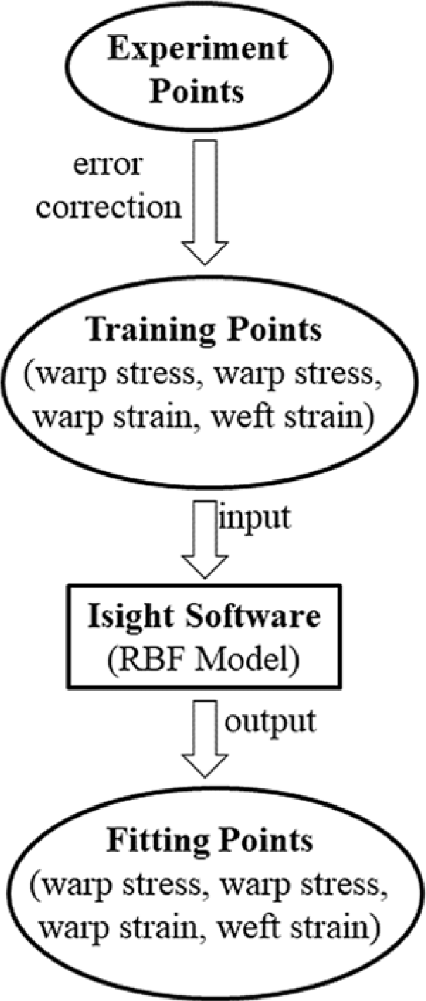
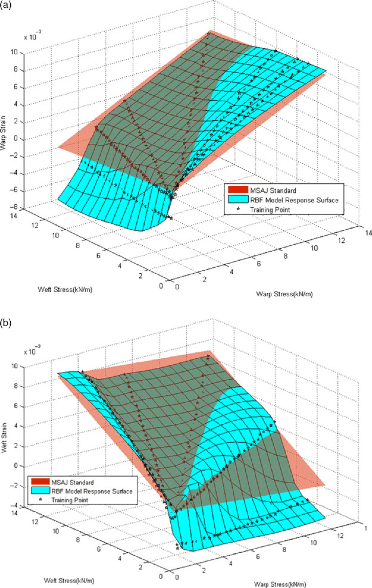
The RBF is a powerful tool to approximate large amounts of scattered data(Reference Hardy30). Since the mesh-free approximation problem is converted to the solution of a linear system(Reference Fasshauer31), the RBF approximation is also efficient for high-dimensional spaces(Reference Li, Deng, Zhang, Yan and Wang32). In engineering applications, the variation of the stress and the stress ratio of a stratospheric airship envelope is very complicated. In the simulation, the least-squares method is not suitable for accurately predicting the material properties of the skin, whereas the RBF model can provide a more accurate stress–strain constitutive relationship based on the biaxial tensile test data. Isight software provides the RBF approximation model, and the response surface can be obtained by inputting experimental data. The simulation process flow is shown in Fig. 8.
Simulation process flow of RBF in Isight software.

The stress–strain constitutive relationship.

After Isight software produces the response surface of the stress–strain constitutive model, the warp and weft directions, as depicted in Fig. 9, can be obtained using MATLAB software. While the pentagrams represent the training points, the transparent surface represents the stress–strain relationship calculated based on the MSAJ standard.
 \begin{equation}\ \ \ \ AE = \frac{1}{N}\sum\limits_{i = 1}^N {(\left| {{Y_i} - F({x_i})} \right|)} \end{equation}
 \begin{equation}\,ME = \max \left\{ {\left| {{Y_i} - F({x_i})} \right|} \right\}\end{equation}
 \begin{equation}\ RMSE = \sqrt {\frac{1}{N}{{\sum\limits_{i = 1}^N} {({Y_i} - F({x_i}))} ^2}} \end{equation}
 \begin{equation}R - Square = 1 - \frac{{{{\sum\limits_{i = 1}^N} {({Y_i} - F({x_i}))} ^2}}}{{\sum\limits_{i = 1}^N {{{({Y_i} - \bar Y)}^2}} }}\qquad\end{equation}
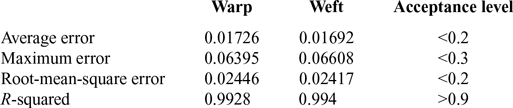
where AE represents the average error, ME represents maximum error, RMSE represents the root-mean-square error, N is the number of samples,
 ${Y_i}(i = 1,...,N)$
are real values,
 $\bar Y$
is the average value of
 ${Y_i}(i = 1,...,N)$
, and
 $F({x_i})(i = 1,...,N)$
are interpolation values. It can be recognised that the accuracy of the model meets the acceptance level requirements.
Using the approximate model established above, the strain in the warp and weft directions can be obtained for different stress ratios. This is a benefit of predicting the deformation of the stratospheric airship envelope under biaxial tensile stress. Compared with the least-squares method, it offers the advantage of higher accuracy and is more suitable for engineering applications. Its disadvantage is that it requires a lot of experimental data and the simulation is more complicated than the least-squares method.
The error analysis for the RBF model

5.0 CONCLUSION
This study describes a biaxial tensile experiment on UN-5100 material, which is used for the envelope of stratospheric airships. An approximate modelling method is used to correct the experimental error, thus generating a more accurate stress–strain curve. A stress–strain constitutive model for UN-5100 material is established by using the RBF approach, which is more adaptable to engineering applications. The following conclusions can be drawn from the work presented herein:
-
1. Under biaxial tension, the elastic parameters of UN-5100 material are greatly affected by the stress and the stress ratio, making the elastic constant unsuitable for describing the deformation of the material because the elastic modulus is continually changing. Also, the stress–strain curve is nonlinear, and the necking phenomenon will develop. Therefore, the theory of plane anisotropy is not well suited for UN-5100 material, strictly speaking. A new theoretical model is needed to describe the constitutive model of stratospheric airship envelopes.
-
2. The least-squares method is suitable for simple predictions of the elastic properties of UN-5100, but at high stress ratios, the accuracy of the biaxial tensile is far lower than engineering standards.
-
3. Comparison of Tables 4 and 5 reveals that the benefit of the approximate method is its ability to describe the stress–strain relationship of skin materials under biaxial tension more accurately. Indeed, the error of the approximate method in Table 4 is minimal. Meanwhile, the MSAJ standard using the least-squares method has its limitations, as the strain is negative in the direction of less stress at higher stress ratios (3:1, 1:3, 4:1 and 1:4), and it can only obtain the overall mechanical properties of envelope materials. Compared with the least-squares method, the approximate model is more suitable for predicting the deformation of UN-5100 under biaxial tensile stress.
These conclusions can be extended to other plain-weave composite materials used on stratospheric airships, or other airship materials that satisfy the plane anisotropy, thus having potential in the field of engineering applications.
ACKNOWLEDGEMENTS
This work was supported by the National Science Foundation of China (grant no. 61733017), National Natural Science Foundation of China (grant no. 51906141) and Shanghai Science Foundation of China (grant no. 18ZR1419000).