1. Introduction
The transition to a low-carbon economy poses a great challenge to investors and entrepreneurs: to avoid a climate crisis and follow a path towards the targets set by the 2015 Paris Agreement, low-carbon infrastructure investment needs to be scaled up substantially beyond the projected business as usual levels (cf. Kreibiehl et al. Reference Kreibiehl, Yong Jung, Battiston, Carvajal, Clapp, Dasgupta, Dube, Jachnik, Morita, Samargandi, Williams and Shukla2022). Ambitious policy-making and financial markets are required to set the necessary incentives and efficiently redirect capital flows from emission-intensive and towards low-carbon investment projects (Campiglio (Reference Campiglio2016)). Investment projections made through scenario analysis (e.g. IEA) and integrated assessment modeling (e.g. IPCC) are conducted with little or no consideration of interactions with financial markets and intermediaries (Farmer et al. (Reference Farmer, Hepburn, Mealy and Teytelboym2015); Battiston et al. (Reference Battiston, Monasterolo, Riahi and van Ruijven2021)).
However, financial markets and intermediaries ultimately determine the cost of capital for investment projects. They hence impact overall profitability and the likelihood that the investment project is actually realized. If financial markets perceive a project to be risky (e.g. due to a high leverage ratio), potential investors and creditors will demand compensation in the form of risk premiums that have to be paid on top of risk-free interest rates. Risk premiums increase capital costs and reduce the returns for the project owner such that the project might not be realized. It is well-known that financial market frictions can slow down capital accumulation (cf. Stiglitz and Weiss (Reference Stiglitz and Weiss1981); Azariadis and Kaas (Reference Azariadis and Kaas2016)) which suppresses output and productivity (Bah and Fang (Reference Bah and Fang2016)). The concept has however not been applied to the context of climate policy-induced transition. In this paper, we study the interaction of financial frictions and climate policy during the policy-induced transition to a low-carbon economy and look at their implication for the effectiveness of climate policy. Climate policies that are designed without understanding the impact of financial frictions on the transition dynamics may fail to meet the intended emission reductions.
Three considerations suggest that financial frictions, faced by firms in nonfinancial sectors, may be particularly relevant to the low-carbon transition. First, the low-carbon transition necessitates a substantial accumulation of capital in the low-carbon sector, whereas the capital stock in the emission-intensive sector will be reduced. The larger the reallocation of investment streams and external finance during the transition the larger the frictions that counteract this reallocation.
Second, the low-carbon sectors that need to accumulate capital start from relatively low levels. When incumbent fossil firms are reluctant to switch to cleaner technologies (cf. Beltramello et al. (Reference Beltramello, Haie-Fayle and Pilat2013)) and continue to rely on their established business models, emission-reducing innovations may need to find their way to the market via freshly founded low-carbon companies. These newcomers are on average smaller than their fossil competitors (Kempa et al. (Reference Kempa, Moslener and Schenker2021), Table 2, supplementary information) and lacking retained earnings to finance investment.Footnote 1 With fewer internal finance available, reliance on external finance drives up leverage ratios and financial risk of the projects. Financial markets price these risks at higher premiums. Furthermore, the relative burden of search and transaction costs associated with the acquisition of external finance is higher for small companies, which are found to be more financially constrained and more unsatisfied with collateral requirements and costs of obtaining external finance (European Central Bank (2020); European Investment Bank (2021)).Footnote 2 The relevance of constrained internal finance increases with the velocity of the transition. Retained earnings only develop over time. The more this transition is rushed, the larger the ratio of external finance to internal finance, i.e. the higher the financial risks that need to be taken to facilitate the transition.
Third, structural differences in the financial characteristics of low-carbon and emission-intensive firms suggest that risk premiums paid by low-carbon companies are more sensitive towards changes in leverage. We identify two potential financial asymmetries that could generate disproportional impacts of financial frictions:
Uncertainty of entrepreneurial success. Low-carbon companies that rely on novel technologies and business models are exposed to additional uncertainties when learning curves, technological limits, and regulation are less known compared to those of conventional companies (Kempa et al. (Reference Kempa, Moslener and Schenker2021)). In cases where these uncertainties translate to higher risk of bankruptcy, lenders will charge larger risk premiums to cover expected losses.
Bankruptcy costs. Low-carbon companies introduce new technologies and thus tend to have a higher innovative capacity than market incumbents on average and thus a higher share of intangible assets. Similarly, they exhibit smaller shares of property, plant, and equipment in total assets.Footnote 3 Intangibles assets are, however, more likely to lose value in case of bankruptcy (Wang et al. (Reference Wang, Forbes, Fenech and Vaz2018); François (Reference François2019)). Risk premiums reflect this relatively larger risk for the clean sectors.
To the best of our knowledge, the constraints that the above arguments put on the ability of nonfinancial firms to acquire finance have not been studied in the context of a sectoral transition. More attention has been paid to the ability of the financial sector to supply finance. Spiganti and Comerford (Reference Spiganti and Comerford2017) and Carattini et al. (Reference Carattini, Heutel and Melkadze2021) show that the sudden introduction of climate policy creates stranded assets that undermine debt capacities of financially constrained investors which constricts the supply of finance to low carbon projects. These studies build on a fast-growing literature on (environmental) dynamic stochastic general equilibrium (E-DSGE) models that study the impact of environmental as well as climate policies (cf. Fischer and Springborn (Reference Fischer and Springborn2011); Heutel (Reference Heutel2012); Argentiero et al. (Reference Argentiero, Bollino, Micheli and Zopounidis2018); Niu et al. (Reference Niu, Yao, Shao, Li and Wang2018)). In contrast to this work, these studies focus on steady state analysis (but see Donadelli et al. (Reference Donadelli, Grüning and Hitzemann2019) for a study of transition risk). All of these E-DSGE studies abstract from financing conditions.
The implications of financial asymmetries between low-carbon and emission-intensive firms are explored in Haas and Kempa (Reference Haas and Kempa2020). The authors use a principal agent model to show how information asymmetries between lenders and potential borrowers that invest in risky renewable energy projects instead of risk-free fossil projects can lead to credit rationing. The authors derive sharp analytical results but do not explore the implications quantitatively. Diluiso et al. (Reference Diluiso, Annicchiarico, Kalkuhl and Minx2020) and Benmir & Josselin, Reference Benmir and Josselin2021) employ E-DSGE models with financial frictions, emissions, and clean and dirty sectors. They implement financial frictions in the banking sector following Gertler and Karadi (Reference Gertler and Karadi2011) and focus the analysis on financial stability, monetary policy, and stranded assets. However, the implications of financial frictions in the nonfinancial production sector on the effect of climate policy have not been studied so far.
In this paper, we addresses the question to what extent financial frictions within nonfinancial sectors undermine the intended effects of climate policy. We specifically consider the joint effects of financial frictions and emission taxes on capital accumulation, and ask what the implications of a delayed and thus rushed climate policy are when financial frictions are present. Finally, we investigate if sectoral responses to macroeconomic shocks are different in the presence of frictions and asymmetries and what the consequences are for the emission intensity of the economy.
The model presented in this paper builds on the financial accelerator approach from Bernanke et al. (Reference Bernanke, Gertler and Gilchrist1999) augmented with sector heterogeneity, emissions, and climate policy. In contrast to the financial frictions mechanism from Gertler and Karadi (Reference Gertler and Karadi2011), this approach offers a natural way to differentiate financial asymmetries between sectors.Footnote 4 Low-carbon and emission-intensive firms are modeled by two groups of intermediate goods producers, clean and dirty, that utilize capital and labor to produce intermediate goods. Emissions are modeled similarly to Fischer and Springborn (Reference Fischer and Springborn2011), i.e. proportional to the output in the dirty sector. Damages from climate change are not modeled.Footnote 5 The economy is subject to an exogenously set emissions tax. We calibrate the model of the Euro area in 2017, accounting for the financial asymmetries outlined above.
We demonstrate the adverse effect of financial frictions and financial asymmetries on the transitional dynamics initiated by a permanent increase in emission taxes. Specifically, we model an emissions tax implemented in 2017, intended to steer the Euro Area towards the achievement of its 2030 mitigation target. We show how frictions undermine the steering effect of the tax, slow down the transition, and increase its costs. If policy makers do not account for the effect of frictions when designing emissions taxes, climate targets will be missed. Our analysis suggests that climate policy ignorant of financial frictions can lead to the Euro Area missing its 2030 climate target by 11 percentage points. That is, relative to 1990, emissions in 2030 are only reduced by 44% instead of the envisaged 55%. We further show how the relevance of financial frictions increases with the delay of climate policy implementation. In 2017, the required emissions tax rate to achieve the 2030 target in an economy subject to financial frictions is 24% above the required tax rate in an economy without financial frictions. If climate policy were to be delayed until for instance 2025, this difference would increase to 37%. Finally, we show how financial frictions in combinations with financial asymmetries impact the transmission mechanism of financial wealth and uncertainty shocks. We discover a risk and a volume effect whose relative strength drives the emission intensity of the economy in the aftermath of shocks.
Our contribution to the literature is threefold. First, we implement financial frictions with the nonfinancial production sector in an E-DSGE model with an emission intense dirty sector and a less emitting clean sector. Second, we employ the financial frictions mechanism from Bernanke et al. (Reference Bernanke, Gertler and Gilchrist1999) which provides more entry points for financial asymmetries than currently used mechanism from Gertler and Karadi (Reference Gertler and Karadi2011). Third, we use company-level data to quantify financial asymmetries between clean and dirty companies and their influence on sectoral performance.
The remainder of this paper is organized as follows: Section 2 introduces the model structure. Section 3 elaborates on the calibration approach and discuss the model fit. Model simulations are evaluated in Section 4. Section 5 concludes the paper.
2. Model Economy
We start by introducing the benchmark model with financial frictions. We provide all equations in the main text but delegate lengthy technical derivations to appendices. The model economy is populated by households, capital goods producers, intermediate good entrepreneurs belonging to either the clean or the dirty sector, a representative capital mutual funds (CMF) for each sector and final goods producers. Households choose consumption, allocate funds to one period deposits with the CMFs, and supply labor to the intermediate goods producing firms managed and owned by entrepreneurs. The entrepreneurs and their firms belong to either the clean or the dirty sector with a sector-specific production technology. We denote sector-affiliated variables and parameters with index
 $i\in \{c,d\}$
where
 $c$
and
 $d$
correspond with the clean and dirty sector, respectively. Rather than classifying entrepreneurs as clean or dirty according to business sectors, we classify them according to their relative emission intensity within their business sector. Intermediates from the same business sectors thus will be part of both, the clean and the dirty sector.Footnote
6
Entrepreneurs own capital stocks, borrow money from CMFs, and sell the output of their companies as intermediate goods to final goods producers. Final goods are used for consumption and investment. Capital goods producers purchase investment goods and old depreciated capital to transform it into new capital to sell to entrepreneurs. In this benchmark economy, financial frictions arise from potential entrepreneurial defaults and associated bankruptcy costs. In order to cover expected nonperforming loans, CMFs will charge risk premiums when extending funds to entrepreneurs. To isolate their effect, we construct an otherwise equivalent frictionless economy, which we describe at the end of this section.
2.1 Households
The economy is populated with infinitely many utility maximizing households. We adopt the large family assumption where each household contains a large and constant number of workers, dirty and clean entrepreneurs such that also the income from entrepreneurial activities belongs to the household ultimately (cf. Christiano et al. (Reference Christiano, Motto and Rostagno2014); Gertler and Karadi (Reference Gertler and Karadi2011)). The representative household maximizes its intertemporal utility by choosing consumption
 $C_{t}$
, labor supply
 $L_{t}$
, and one-period deposits
 $D_{t+1}$
Footnote
7
at the CMF. Bank deposits are risk-free assets paying an ex post real return
 $R_{t+1}$
. The households’ lifetime utility is
 \begin{equation*} U_{t}=\sum _{t=0}^{\infty }\beta ^{t} u\left ( C_{t},L_{t}\right ) \ \mbox {with}\ u(C_t,L_t)=\log \left ( C_{t}\right ) +\log \left ( 1-L_{t}\right ) \end{equation*}
where
 $\beta$
is the discount factor. Consumption and savings are financed by labor income
 $w_{t}L_{t}$
, interest-bearing deposits from the previous period
 $R_{t}D_{t}$
, lump-sum tax transfers
 $T_{t}$
, and net transfers from entrepreneurs
 $M_{t}$
. This yields the following budget constraint:
 \begin{equation*} C_{t}+D_{t+1}=w_{t}L_{t}+R_{t}D_{t}+T_{t}+M_{t} \end{equation*}
with
 \begin{equation*} M_{t}=C_{dt}+C_{ct}-M_{d}-M_{c} \end{equation*}
Net transfers from entrepreneurs
 $M_{t}$
consist of entrepreneurial wealth from the clean sector
 $C_{ct}$
and dirty sector
 $C_{dt}$
and seed finance to entrepreneurs in both sectors,
 $M_{c}$
and
 $M_{d}$
. The exact characteristics of transfer payments are provided in Section 2.3.
2.2 Final goods production
A representative, perfectly competitive final goods producer combines intermediate dirty goods
 $Y_{dt}$
and intermediate clean goods
 $Y_{ct}$
into a final good
 $Y_{t}$
used for consumption and investment. The final goods producer purchases the intermediate output from the dirty and clean sector at prices
 $p_{dt}$
and
 $p_{ct}$
, respectively. The price of the final good is normalized to one. Production uses standard constant elasticity of substitution technology:
 \begin{equation*} Y_{t}=z_{At}A\left [ \phi Y_{dt}^{1-\varepsilon }+\left ( 1-\phi \right ) Y_{ct}^{1-\varepsilon }\right ] ^{\frac {1}{1-\varepsilon }} \end{equation*}
where
 $A$
is constant total factor productivity,
 $z_{At}$
is a shock process,
 $\phi$
is a share parameter, and
 $\varepsilon$
is the inverse of the elasticity of substitution between dirty and clean intermediate goods.
2.3 Entrepreneurs and intermediate goods production
Intermediate goods are produced by identical, perfectly competitive firms belonging to either the dirty sector
 $d$
or the clean sector
 $c$
. Dirty and clean firms are owned and managed by entrepreneurs
 $j$
that are heterogeneous with respect to the levels of their net worth. Bank loans (external finance) and entrepreneurial net worth (internal finance) are the two sources of funds that firms use to finance operations. Entrepreneurial net worth positions thus change with retained earnings. At the end of period
 $t-1$
, entrepreneur
 $j$
is characterized by his level of net worth
 $N_{it}^{j}$
where
 $i\in \{d,c \}$
denotes sector affiliation.Footnote
8
Entrepreneurs maximize period
 $t$
profits in two steps: they first decide the amount of capital to purchase, before learning the true productivity of their technology. Second, they decide the level of labor, which is chosen as the optimal complement to the capital once the entrepreneurs have learned their productivity.
To determine optimal capital acquisition in the first step, entrepreneurs decide on the loan volume
 $B_{it}^{j}$
obtained from the CMF to combine it with their net worth
 $N_{it}^{j}$
and the amount of capital
 $K_{it}^{j}$
to buy at market price
 $Q_{it-1}$
at the end of period
 $t-1$
.Footnote
9
 \begin{equation} Q_{it-1}K_{it}^{j}=B_{it}^{j}+N_{it}^{j} \end{equation}
The first-order conditions that determine the choice of
 $B_{it}^j$
are detailed in a financial contract between entrepreneurs and CMF as described in Section 2.4 below. At the beginning of period
 $t$
, entrepreneurs learn their idiosyncratic productivity
 $\omega _{it}^{j}$
and hence their effective capital stock
 $\bar{K}_{it}^{j}=\omega _{it}^{j}K_{it}^{j}$
. The productivity shocks
 $\omega _{it}^{j}$
are unit mean and log-normally i.i.d. variables with standard deviation
 $z_{\sigma t}\sigma _{i}$
. The stochasticity of effective capital captures the volatility of entrepreneurial success, e.g. due to market trends or the adoption of technological standards. The standard deviation
 $z_{\sigma t}\sigma _{i}$
is subject to a risk shock
 $z_{\sigma t}$
, capturing that the riskiness of entrepreneurs’ production changes over time (Christiano et al. (Reference Christiano, Motto and Rostagno2014)). The dynamics of the risk shock are characterized below. The probability density function of
 $\omega _{it}^{j}$
is denoted by
 $f( \omega _{it}^{j})$
and the cumulative distribution function by
 $F( \omega _{it}^{j})$
.
In the second step, once they have learned the level of their effective capital stock
 $\bar{K}_{it}^{j}$
, entrepreneurs decide how much labor
 $L_{it}^{j}$
to hire as the second input to their intermediate goods technology
 $Y_{it}^{j}$
.
 \begin{equation} Y_{it}^{j}=A_{i}\left ( \bar{K}_{it}^{j}\right ) ^{\alpha _{i}}\left ( L_{it}^{j}\right ) ^{1-\alpha _{i}} \end{equation}
The constant
 $A_{i}$
expresses sectoral productivity, output elasticities of capital, and labor are denoted by
 $\alpha _i$
and
 $( 1-\alpha _{i})$
, respectively. Entrepreneurs can only access the production technology of their sector and pay
 $w_{t}$
for each unit of labor employed. The production of
 $Y_{it}^{j}$
is associated with
 $\xi _{i}Y_{it}^{j}$
emissions of greenhouse gases. Parameter
 $\xi _{i}$
denotes the emission intensity of the production technology within sector
 $i$
. Intermediate goods are sold to final goods producers at price
 $p_{it}$
. Emissions are taxed
 $\tau _{it}^{E}$
. Entrepreneurs sell their depreciated capital stock
 $ ( 1-\delta ) \bar{K}_{it}^{j}$
back to capital goods producers at price
 $\bar{Q}_{it}$
. The depreciation rate is denoted by
 $\delta$
. Ultimately, the gross return on capital to entrepreneur
 $j$
is composed of revenues from selling intermediate goods to final goods producers, the depreciated capital stock to capital goods producers, less taxes and wages:
 \begin{equation} \Pi _{it}^{j}=\left ( p_{it}-\xi _{i}\tau _{it}^{E}\right ) Y_{it}^{j}-w_{t}L_{it}^{j}+\bar{Q}_{it}\left ( 1-\delta \right ) \bar{K}_{it}^{j} \end{equation}
At this point, entrepreneurs’ effective capital stocks
 $\bar{K}_{it}^{j}$
are fixed (first step profit maximization) and the maximization of the gross return on capital with respect to labor (second step profit maximization) yields
 \begin{equation} w_{t}=\left ( p_{it}-\xi _{i}\tau _{it}^{E}\right ) \frac{\partial Y_{it}^{j}}{\partial L_{it}^{j}} \end{equation}
such that entrepreneurial gross returns on capital can be expressed asFootnote 10
 \begin{equation*} \Pi _{it}^{j}=R_{it}^{k}Q_{it-1}\omega _{it}^{j}K_{it}^{j} \end{equation*}
where
 $R_{it}^{k}$
is the average gross rate of return on capital across sector
 $i$
entrepreneurs in
 $t$
and defined as
 \begin{equation*} R_{it}^{k} = \frac {\left ( p_{it}-\xi _{i}\tau _{it}^{E}\right ) \alpha _{i} \left ( A_{i}^{\frac {1}{1-\alpha _{i}}}\left ( 1-\alpha _{i}\right ) \frac {p_{it}-\xi _{i}\tau _{it}^{E}}{w_{it}} \right )^{\frac {1-\alpha _{i}}{\alpha _{i}}} +\left ( 1-\delta \right ) \bar {Q}_{it}}{Q_{it-1}} \end{equation*}
The first term of the sum is the marginal product of capital in the production function of sector
 $i$
entrepreneurs, relative to the gross price for which they purchased capital. The second term represents the value appreciation or depreciation of capital. Entrepreneurs obtain external finance in the form of one-period loans from the CMF where a standard debt contract stipulates a loan amount
 $B_{it}^{j}$
and interest rate
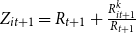
 $Z_{it}^{j}$
to be repaid by borrowers after the disposal of intermediate goods and depreciated capital stocks. The financial contract is derived in Appendix B. Entrepreneurs only repay the loan when they can, i.e. they have non-negative equity after debt repayment. This implies a minimum productivity level
 $\bar{\omega }_{it}^{j}$
that entrepreneurs need in order to repay their debt. This cutoff productivity or bankruptcy threshold is defined as follows:
 \begin{equation} R_{it}^{k}Q_{it-1}\bar{\omega }_{it}^{j}K_{it}^{j}=Z_{it}^{j}B_{it}^{j} \end{equation}
If
 $\omega _{it}^{j}\gt \bar{\omega }_{it}^{j}$
, the entrepreneur repays the lender
 $Z_{it}^{j}B_{it}^{j}$
and keeps the equity
 $(\omega _{it}^{j}-\bar{\omega }_{it}^{j})R_{it}^{k}Q_{it-1}K_{it}^{j}$
. The entrepreneur defaults for values
 $\omega _{it}^{j}\lt \bar{\omega }_{it}^{j}$
in which case the CMF claims the entrepreneur’s assets and the entrepreneur end up with
 $V_{it}^j=0$
.Footnote
11
Bankruptcy is costly (Hotchkiss et al. (Reference Hotchkiss, John, Thorburn and Mooradian2008), cf.) and CMFs have to incur bankruptcy cost
 $\mu _i$
when claiming a defaulting entrepreneur’s assets. We assume bankruptcy costs are proportional to gross return on capital and the CMF can claim
 $ ( 1-\mu _{i} ) \omega _{it}^{j}R_{it}^{k}Q_{it-1}K_{it}^{j}$
. Therefore, before knowing the precise size of the productivity shock
 $\omega _{it}^{j}$
, the expected individual entrepreneurial equity is given by
 \begin{equation*} E_{t-1}\left [V_{it}^{j}\right ] = E_{t-1}\left [z_{Vt}\left ( R_{it}^{k}Q_{it-1}\int _{\bar {\omega }_{it}^{j}}^{\infty }\omega _{it}dF\left ( \bar {\omega }_{it}^{j}\right ) K_{it}^{j}-Z_{it}^{j}B_{it}^{j}\left [ 1-F\left (\bar {\omega }_{it}^{j}\right ) \right ] \right ) \right ] \end{equation*}
Similar to Christiano et al. (Reference Christiano, Motto and Rostagno2014), we introduce a financial wealth shock
 $z_{Vt}$
to entrepreneurial equity positions which effects entrepreneurs indiscriminately of sector affiliation. Shock dynamics are characterized in Section 2.7. Substituting equation (5) allows to eliminate
 $Z_{it}^{j}B_{it}^{j}$
.
 \begin{eqnarray} E_{t-1}\left [V_{it}^{j}\right ]&=&E_{t-1}\left [ z_{Vt}R_{it}^{k}l_{it}^{j}N_{it}^{j}\left [ 1-\Gamma \left ( \bar{\omega }_{it}^{j}\right ) \right ] \right ] \end{eqnarray}
Here,
 $l_{it}^{j}$
denotes leverage and is defined as the purchase value of entrepreneurial capital stock divided by current net worth
 \begin{equation} l_{it}^{j}=\frac{Q_{it-1}K_{it}^{j}}{N_{it}^{j}} \end{equation}
and
 $\Gamma ( \bar{\omega }_{it}^{j} ) =\int _{0}^{\bar{\omega }_{it}^{j}}\omega _{it}dF ({\omega }_{it}^{j} ) +\bar{\omega }_{it}^{j} [ 1-F ( \bar{\omega }_{it}^{j} ) ]$
represents the gross share of profits going to the lender such that the share of average entrepreneurial earnings that remains with the entrepreneur corresponds to
 $1-\Gamma ( \bar{\omega }_{it}^{j} )$
.Footnote
12
For the discussion of simulation results, we consider a more intuitive measure of leverage, the debt-to-assets ratio which we refer to as leverage ratio and define it as
 \begin{equation*} lr_{it}^{j}=\frac {B_{it}^{j}}{Q_{it-1}K_{it}^{j}}=1-\frac {1}{l_{it}^{j}} \end{equation*}
After loan repayment, end-of-period
 $t$
entrepreneurial net worth
 $N_{it+1}^{j}$
is determined. At any
 $t$
, a share
 $1-\nu _{i}$
of entrepreneurs liquidate their firms and become working members of their household. Each period, a sufficient amount of workers become entrepreneurs such that the number of entrepreneurs is constant. Upon firm liquidation, entrepreneurs transfer their wealth in the form of consumption
 $C_{it}$
to households as part of their “large family.” Households in turn provide seed finance
 $M_{i}$
to entrepreneurs in every period. These assumptions reflect that entrepreneurs enter and exit the economy, frequently invest their individual wealth and always rely on external finance to some extent. A share
 $\nu _{i}$
of entrepreneurs continue operating their businesses such that individual entrepreneurial net worth
 $N_{it+1}^{j}$
of the remaining and new entrepreneurs is given by
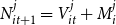 $N_{it+1}^{j}=V_{it}^{j}+M_{i}^{j}$
. Aggregate net worth is given by
 $N_{it+1}=\nu _{i}V_{it}+M_{i}$
and Appendix C shows that this corresponds to:
 \begin{align} N_{it+1}=\nu _{i}z_{Vt}\left [ \left ( R_{it}^{k}Q_{it-1}K_{it}-\left \{ R_{t}+\frac{\mu _{i}G\left ( \bar{\omega }_{it}\right ) R_{it}^{k}Q_{it-1}K_{it}}{Q_{it-1}K_{it}-N_{it}}\right \} \left ( Q_{it-1}K_{it}-N_{it}\right ) \right ) \right ] +M_{i} \end{align}
The net worth is then used together with fresh loans
 $B_{it+1}^{j}$
to purchase next periods capital stock
 $K_{it+1}^{j}$
and then move on to the next period.
2.4 Financial intermediation
The loans required by entrepreneurs in order to purchase capital are provided by households through perfectly competitive CMFs. We model this by a representative CMF who, at the end of period
 $t$
, takes deposits
 $D_{t+1}$
at interest rate
 $R_{t+1}$
from households and extends one-period loans
 $B_{it+1}^{j}$
to entrepreneur
 $j$
belonging to sector
 $i$
according to an optimal financial contract. The contract is characterized by loan volume
 $B_{it+1}^{j}$
and a gross nondefault loan rate
 $Z_{it+1}^{j}$
. The loans are retired at the end of the subsequent period. Perfect competition and the assumption of free entry gives rise to the following zero-profit condition for the representative CMF.
 \begin{equation*} \left [ 1-F\left ( \bar {\omega }_{it+1}^{j}\right ) \right ] Z_{it+1}^{j}B_{it+1}^{j}+\left ( 1-\mu _{i}\right ) R_{it+1}^{k}Q_{it}\int _{0}^{\bar {\omega }_{it+1}^{j}}\omega _{it+1}dF\left ( \omega _{it+1}^{j}\right ) K_{it+1}^{j}=R_{t+1} B_{it+1}^{j} \end{equation*}
The left-hand side represents the expected return on the loan provided to entrepreneur
 $j$
. The first term on the left-hand side corresponds to the payment received from nondefaulting entrepreneur
 $j$
and the second term corresponds to the payment received in case of default net of bankruptcy costs. The right-hand side is equivalent to the opportunity cost of funds. There are two opposing effects of changing entrepreneurial interest rates with respect to the zero-profit condition: Increasing
 $Z_{it+1}^j$
yields higher nondefault payments from the entrepreneurs who can repay their debt but also rises the default probability which reduces the amount of entrepreneurs that are able to repay loans and vice versa. Substituting equation (5) allows to express the zero- profit condition in terms of
 $B_{i,t}^{j}$
and
 $\bar{\omega }_{i,t}^{j}$
:
 \begin{equation*} \left ( \left [ 1-F\left ( \bar {\omega }_{it+1}^{j}\right ) \right ] \bar {\omega }_{it+1}^{j}+\left ( 1-\mu _{i}\right ) \int _{0}^{\bar {\omega }_{it+1}^{j}}\omega _{it+1}dF\left ( \omega _{it+1}^{j}\right ) \right ) R_{it+1}^{k}Q_{it}K_{it+1}^{j}=R_{t+1}B_{it+1}^{j} \end{equation*}
Substituting (1) and (7) and rearranging allows
 \begin{equation} \left [ \Gamma \left ( \bar{\omega }_{it+1}^{j}\right ) -\mu _{i}G\left ( \bar{\omega }_{it+1}^{j}\right ) \right ] R_{it+1}^{k}l_{it+1}^{j}= R_{t+1}\left ( l_{it+1}^{j}-1\right ) \end{equation}
where, if
 $\Gamma ( \bar{\omega }_{it+1}^{j} )$
represents the gross share of entrepreneurial profits going to the lender as above, the net share of profits going to the lender equals
 $\Gamma ( \bar{\omega }_{it+1}^{j} ) -\mu _{i}G ( \bar{\omega }_{it+1}^{j} )$
and
 $G ( \bar{\omega }_{it+1}^{j} ) =\int _{0}^{\bar{\omega }_{it+1}^{j}}\omega dF ( \omega _{it+1} )$
. The combinations of
 $ ( \bar{\omega }_{it+1}^{j},l_{it+1}^{j} )$
that are implied by the zero- profit condition define a range of contingent standard debt contracts of which the entrepreneur will choose the one that maximizes expected return from equation (6). This optimization is the first step in the profit maximization of entrepreneurs. The solution is derived in Appendix B and consists of the optimality condition
 \begin{equation} 0=\frac{R_{it+1}^{k}}{ R_{t+1}}\left [ 1-\Gamma \left ( \bar{\omega }_{it+1}\right ) \right ] +\frac{\Gamma ^{\prime }\left ( \bar{\omega }_{it+1}\right ) }{\Gamma ^{\prime }\left ( \bar{\omega }_{it+1}\right ) -\mu _{i}G^{\prime }\left ( \bar{\omega }_{it+1}\right ) }\left ( \left [ \Gamma \left ( \bar{\omega }_{it+1}\right ) -\mu _{i}G\left ( \bar{\omega }_{it+1}\right ) \right ] \frac{R_{it+1}^{k}}{ R_{t+1}}-1\right ) \end{equation}
and the aggregated zero-profit condition for CMFs:
 \begin{equation} \left [ \Gamma \left ( \bar{\omega }_{it+1}\right ) -\mu _{i}G\left ( \bar{\omega }_{it+1}\right ) \right ] R_{it+1}^{k}l_{it+1}= R_{t+1}\left ( l_{it+1}-1\right ) \end{equation}
The term
 $\frac{R_{it+1}^{k}}{ R_{t+1}}$
in equation (10) describes the return a unit of capital has to generate, discounted by the interest rate demanded by households. If above one, it can be thought of as an external finance premium the entrepreneur has to pay on top of the risk-free rate.Footnote
13
Note that
 $j$
-specific variables vanished from equations (10) and (11), i.e. all entrepreneurs within a sector will choose a financial contract which allows them to sustain the same optimal leverage ratio (yielding identical cutoff productivities
 $\bar{\omega }_{it+1}$
), irrespective of their heterogeneous net worth positions. Entrepreneurs with minor net worth positions will thus borrow less than entrepreneurs with larger net worth positions such that leverage ratios are identical. It is the external financing premium that harmonizes optimal leverage ratios across individual entrepreneurs.Footnote
14
Entrepreneurs within a sector operate perfectly competitive firms and exhibit identical expected efficiencies (the financial contract is concluded prior to the realization of the next productivity shock).Footnote
15
Appendix B shows that equation (11) can be condensed to:
 \begin{equation} \frac{R_{it+1}^k}{R_{t+1}}=s_i(l_{it+1}) \end{equation}
with
 $s_i'(l_{it+1})\geq 0$
. It is now obvious that increasing leverage rises external finance premiums charged by CMFs. The severity of the increment is mainly driven by the financial characteristics of entrepreneurs (uncertainty
 $\sigma _i$
and bankruptcy cost
 $\mu _i$
) which are parameters to the function
 $s(\!\cdot\!)$
.
2.5 Capital goods producers
Within each sector, there are perfectly competitive capital goods producers that buy the old, depreciated capital stock of intermediate goods producers
 $ ( 1-\delta ) K_{it}$
at real price
 $\bar{Q}_{it}$
. They then combine it with investment goods
 $I_{it}$
and produce capital stock for production processes in the next period
 $K_{it+1}$
sold to entrepreneurs at price
 $Q_{it}$
. Capital goods producers’ profits are
 \begin{equation*} \Pi _{it}^{I}=Q_{it}K_{it+1}-I_{it}-\frac {\chi }{2}\left ( \frac {I_{it}}{K_{it}}-\delta \right ) ^{2}K_{it}-\bar {Q}_{it}\left ( 1-\delta \right ) K_{it} \end{equation*}
where
 $p_{t}$
is the price of the numeraire and normalized to one,
 $\chi$
determines investment adjustment costs. Capital evolves according to:
 \begin{equation*} K_{it+1}=\left ( 1-\delta \right ) K_{it}+I_{it} \end{equation*}
The capital goods producers’ profit maximization yields the following levels for capital pricesFootnote 16 :
 \begin{eqnarray*} Q_{it} &=&\left (1+\chi \left ( \frac{I_{it}}{K_{it}}-\delta \right ) \right ) \\[5pt] \bar{Q}_{it} &=&Q_{it}-\frac{1}{1-\delta }\left [ \frac{\chi }{2}\left ( \frac{I_{it}}{K_{it}}-\delta \right ) ^{2}-\chi \left ( \frac{I_{it}}{K_{it}}-\delta \right ) \frac{I_{it}}{K_{it}}\right ] \end{eqnarray*}
2.6 Government
In this model, the government sets the level of taxes in order to reach an exogenous climate target. This exogenous target reflects for the short-term time horizon that we model, the feedback of greenhouse gas emissions and climate change impacts will not be decisive for climate policy due to the delays and inertia of the climate system and the limited influence of emissions from the Euro Area on global greenhouse gas concentration. Acknowledging that emissions are proportional to dirty intermediate output, the tax
 $\tau _{t}^{E}$
can be interpreted as a price on emissions. The government ensures a balanced budget each period, i.e. all tax revenues are rebated in a lump-sum transfer
 $T_t$
to households:
 \begin{equation*} T_{t}=\tau _{t}^{E}(\xi _{c}Y_{ct}+\xi _{d}Y_{dt}) \end{equation*}
2.7 Shocks
We consider three structural shocks: a shock to total factor productivity
 $z_{At}$
, the risk shock
 $z_{\sigma t}$
, and a shock to entrepreneurial net worth positions
 $z_{Vt}$
. Shocks are modeled as log deviations from steady-state values in the form of univariate first-order autoregressive processes:
 \begin{equation*} \log x_{t}=\rho _{x}\log x_{t-1}+\varepsilon _{xt} \end{equation*}
where
 $x_{t}$
is the innovation,
 $\rho _{x }\in (0,1)$
measures persistence of the shock and
 $\varepsilon _{xt}$
is normally distributed, zero-mean white noise with standard deviation
 $\sigma _{x}$
. We follow the standard assumption that statistical innovations of shocks are learned by agents at the time the innovation materializes.
2.8 Market clearing
The aggregate resource constraint is given by the goods market clearing.
 \begin{align} Y_{t} &= C_{t}+I_{ct}+I_{dt}\nonumber \\ &\quad +\mu _{c}G\left ( \bar{\omega }_{ct}\right ) R_{ct}^{k}Q_{ct-1}K_{ct} +\mu _{d}G\left ( \bar{\omega }_{dt}\right ) R_{dt}^{k}Q_{dt-1}K_{dt} \end{align}
 \begin{align} &+\frac{\chi }{2}\left ( \frac{I_{ct}}{K_{ct}}-\delta \right ) ^{2}K_{ct}+\frac{\chi }{2}\left ( \frac{I_{dt}}{K_{dt}}-\delta \right ) ^{2}K_{dt} \end{align}
Line (13) corresponds to the bankruptcy costs of the two sectors and line (14) to the investment adjustment costs. Labor and debt market clearing imply
 \begin{eqnarray*} L_{t} &=&L_{ct}+L_{dt} \\[5pt] D_{t+1} &=& B_{ct+1}+ B_{dt+1} \end{eqnarray*}
2.9 Frictionless economy
When simulating the behavior of the benchmark economy in response to shocks, we compare the results to the behavior of the frictionless economy. Frictions are eliminated by setting
 $\mu _i=0$
, ensuring that banks can learn entrepreneurs’ idiosyncratic productivity without any cost. Without the existence of bankruptcy costs, CMFs charge no risk premiums on top of the risk-free rate and
 $R^k_i= R_{t+1}$
. Rearrange equation (8) in steady state to see that mainly transfers from households determine entrepreneurial net worth.
 \begin{equation*} N_i=\frac {M_i}{1-vz_{vt}R} \end{equation*}
Given minuscule transfers, entrepreneurs have close to zero net worth. But in the absence of risk premiums, entrepreneurs can disregard net worth and take highly leveraged positions with high bankruptcy probabilities. CMFs can recover the full value of assets from defaulted entrepreneurs and are thus able to perfectly diversify entrepreneurial idiosyncratic risk by charging high-interest rates. The frictionless economy exhibits high-interest rates, high bankruptcy probabilities, minuscule net worth positions, and leverage ratios close to one. Without the small fraction of entrepreneurs for which
 $\omega ^j_i\gt \bar{\omega }^j_i$
and who accumulate net worth, seed finance
 $M_i$
would be the only source of funding for entrepreneurs. Despite the substantial difference in financial variables, the frictionless economy generates a steady state with nonfinancial variables close to the benchmark economy.
3. Calibration and Fit
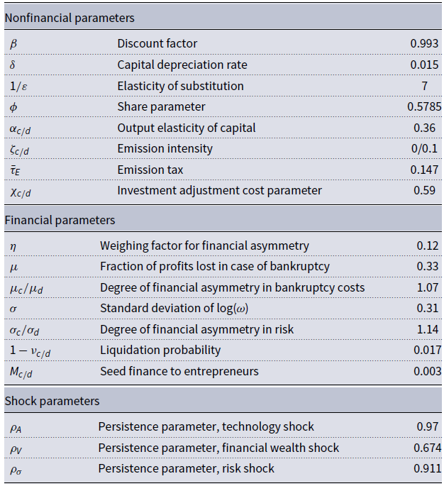
For the numerical analyses, we calibrate the model to the Euro area in 2017. Standard parameters are taken from studies with similar model structure (in particular (Christiano et al. (Reference Christiano, Motto and Rostagno2010); Donadelli et al. (Reference Donadelli, Grüning and Hitzemann2019)), parameters that are specific to the Euro Area are calibrated using data from the AMECO database (European Commission (2021a)), Eurostat (European Commission (2021b)), and the European Central Bank (European Central Bank (2020)). Section 3.1 discusses nonfinancial parameters. In Section 3.2, we apply the calibration approach of Su (Reference Su2019) and use firm-level data from EIKON (Refinitiv (2020)) to estimate financial parameters which reflect the financial asymmetries between the clean and dirty sector. All parameter values are reported in Table 1. Section 3.3 evaluates the fit of the model economy in comparison with its empirical counterparts.
Calibrated parameters (time unit of model: quarter)

3.1 Non-financial parameters
The quarterly household discount factor
 $\beta$
is set to 0.993 and is within conventional ranges (cf. Smets and Wouters (Reference Smets and Wouters2003); Christiano et al. (Reference Christiano, Motto and Rostagno2010)). Data from the AMECO database suggest a quarterly depreciation rate
 $\delta$
of 1.46%. We set the elasticity of substitution between clean and dirty goods
 $1/\epsilon$
to 7 which is at the high end of the range of Acemoglu et al. (Reference Acemoglu, Aghion, Bursztyn and Hemous2012). The high value reflects our sector definition where both sectors produce similar intermediate goods. We set the share parameter
 $\phi$
to 0.5725 such that the fraction of clean intermediate goods in total intermediate goods production fits the data discussed in Section 3.3. The output elasticity of capital
 $\alpha _{i}$
is adopted from Christiano et al. (Reference Christiano, Motto and Rostagno2010). We follow Donadelli et al. (Reference Donadelli, Grüning and Hitzemann2019) and set the emission intensity for the clean sector to zero and to 0.1 for the dirty sector. Steady-state emission taxes are calibrated to generate tax revenues equal to 2.4% of GDP (i.e.
 $\bar{\tau }_E$
= 0.147) which corresponds to the data discussed in Section 3.3. Parameter
 $\chi _{c/d}$
governs the severeness of investment adjustment costs. We use the value from Christensen and Dib (Reference Christensen and Dib2008). Persistence parameters
 $\rho _A$
,
 $\rho _V$
, and
 $\rho _\sigma$
that guide the impact of shocks on the economy are taken from Christiano et al. (Reference Christiano, Motto and Rostagno2010).
3.2 Financial parameters
The relevance of frictions increases along with three financial characteristics: liquidation probability (
 $1-\nu _i$
), bankruptcy cost (
 $\mu _i$
), and uncertainty about entrepreneurial success (
 $\sigma _i$
). For the liquidation probability
 $1-\nu$
, we use the death rates of entrepreneurs in the Euro Area as a proxy, for which the European Commission (2021b) reports a value of 1.7% for 2017. We assume the same liquidation probability for both sectors, i.e.
 $\nu _i=\nu$
. Bankruptcy cost
 $\mu$
and uncertainty about entrepreneurial success
 $\sigma$
are however distinct in both sectors. We first derive economy-wide aggregate values of
 $\mu$
and
 $\sigma$
for the Euro Area from data. We then use the calibration approach from Su (Reference Su2019) to approximate the degree of financial asymmetry in bankruptcy costs and uncertainty. We calculate the degree of financial asymmetry in bankruptcy costs as
 $\mu _c/\mu _d$
and likewise
 $\sigma _c/\sigma _d$
for success uncertainty. In the following paragraphs, we discuss the estimation and calibration for
 $\mu$
and
 $\mu _i$
. The same procedure was followed to calibrate
 $\sigma$
and
 $\sigma _i$
.
The aggregate share of profits lost in bankruptcy
 $\mu$
is approximated by one minus the recovery rate. Recovery rates measure the percentage of a loan recovered by secured creditors through judicial reorganization, liquidation, or debt enforcement. The World Bank (2021a) reports estimates for the countries in the Euro Area. We use a weighted average over countries where weighing factors are gross issues of debt securities per country extracted from the European Central Bank (Securities Issues Statistics (SEC) (2020)) and then average over the years 2013−2017. Uncertainty
 $\sigma$
is set to 0.33 such that the model mirrors the macroeconomic characteristics discussed in Section 3.3, especially debt-to-equity ratios and external finance premiums.
We assume that economy-wide aggregate values for financial parameters
 $\mu$
and
 $\sigma$
relate to sector-specific values in the following way: aggregate values are the averages of sector level values weighted by the market share of the sectors. Formally, when
 $\eta =Y_c/(Y_c+Y_d)$
represents the clean market share then aggregates are defined as follows.
 \begin{equation} \mu = \eta \mu _c+(1-\eta )\mu _d \end{equation}
To our knowledge, there exists no data set which applies our sector definition and reports data on financial parameters bankruptcy cost
 $\mu _i$
and success uncertainty
 $\sigma _i$
aggregated over sectors. We follow the calibration approach from Su (Reference Su2019) where we invert the equations governing the financial part of the model, fix endogenous observable variables to their empirical values obtained from Refinitiv (2020), and then quantify
 $\mu _i$
and
 $\sigma _i$
. We assume that the data represents a steady state and hence omit time indices for the remainder of the section.
Following Su (Reference Su2019), we construct a system of four equations. For the first equation, we rearrange (5):Footnote 17
 \begin{equation} \frac{Z_{i}}{R}=\bar{\omega }_{i}\frac{R_{i}^{k}}{R}\frac{l_{i}}{l_{i}-1} \end{equation}
The second and third equations are equations (10) and (11) from Section 2.4. Equation (23) from Appendix D is the fourth equation:
 \begin{equation} F\left ( \bar{\omega _i}\right ) =\Phi \left [ \frac{\log \bar{\omega _i}+\frac{\sigma _{xi}^{2}}{2}}{\sigma _{xi}}\right ] \end{equation}
This equation expresses default probability where
 $\Phi$
is the cumulative distribution function of the standard normal distribution. In the system (10), (11), (16), and (17), we fix leverage
 $l_{i}$
, default probability
 $F (\bar{\omega }_{i} )$
, and credit spread
 $Z_{i}/R$
to empirical values. This allows us to quantify four (now) endogenously determined variables: cutoff productivity
 $\bar{\omega }_{i}$
, risk premium
 $R_{i}^{k}/R$
, bankruptcy cost
 $\mu _i$
, and success uncertainty
 $\sigma _i$
. We use these estimates to calculate the degree of financial asymmetry
 ${\mu _c}/\mu _d$
as described above. We then use the degrees of financial asymmetry
 ${\mu _c}/\mu _d$
and equation (15) to compute
 $\mu _c$
and
 $\mu _d$
relative to the aggregate value for bankruptcy cost
 $\mu$
(and likewise for
 $\sigma _i$
):
 \begin{eqnarray*} \mu _d &=& \frac{\mu }{\eta \frac{\mu _c}{\mu _d}+(1-\eta )} \\[5pt] \mu _c &=& \frac{\mu \frac{\mu _c}{\mu _d}}{\eta \frac{\mu _c}{\mu _d}+(1-\eta )} \end{eqnarray*}
To gather the estimates for leverage
 $l_i$
, spreads
 $Z_i/R$
, and default probabilities
 $F(\bar{\omega }_i)$
, we consult the data base EIKON ((Refinitiv (2020)), data sets: equities, fixed income) and construct a data set for firms in the Euro Area over the period 2013−2017. We restrict the data set to nonfinancial firms and collect emissions data to allocate firms to the clean and dirty sectors. Emission intensities are calculated as estimated
 $\text{CO}_2$
equivalent emissions divided by total revenue. Since the availability of historical emissions data is limited in EIKON, we use emissions data from 2019. A company whose emission intensity is below the median emission intensity of all companies within the same industry (following The Refinitiv Business Classification) is considered part of the clean sector and otherwise the dirty sector. We cluster companies into industries in order to avoid a comparison of industries with each other but to compare firms within the same industry instead. This is in line with the sector definition in Section 2, and guarantees that firms are allocated to the clean and dirty sector within each industry. Without clustering, all firms from a relatively emission intense industry (e.g. transportation) are allocated to the dirty sector and firms from a less emission intense industry (e.g. IT services) to the clean sector. Resulting differences in financial parameters are then more likely due to industry-specific characteristics instead of environmental performance. In line with Su (Reference Su2019), financial leverage is calculated as total long-term debt divided by total equity. Sectoral leverage
 $l_i$
is calculated by taking the median leverage per sector per year and then averaging over time. Bond spreads serve as a proxy for interest rate spreads of bank loans. Spreads are calculated as the difference in coupon rates of corporate bonds with a 2-, 5- or 10-year maturity and German government bonds of equal maturity. We calculate the median spread per sector of all bond issuances within a month per sector, average over time, and calculate quarterly spreads. Corporate default probabilities are obtained from the StarMine Combined Credit Risk Model (through EIKON) which indicates the probability that the company will go bankrupt, or default on its debt obligations over the next 1-year period. We take median probabilities of all firms within a sector per year, average over time, and calculate quarterly probabilities.
The resulting degree of financial asymmetries is reported in Table 1. Bankruptcy costs and success uncertainty in the clean sector are 107% and 113% of their counterparts in the dirty sector. Final values for
 $\mu _i$
and
 $\sigma _i$
are reported in Table 2 (rows 6 and 7). We choose an infinitesimal small value for the transfer of funds from households to entrepreneurs
 $M_{i}$
as to not generate an additional significant source of net worth.
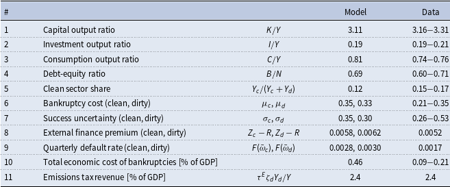
Steady state moments

Ranges represent minimum and maximum values in the years from 2013−2017 or ranges found in the literature. Data sources by rows: 1−3: European Commission (2021a); 4−5, 11: European Commission (2021b); 6: World Bank (2021a, Doing Business); 7: Bernanke et al. (Reference Bernanke, Gertler and Gilchrist1999), Christiano et al. (Reference Christiano, Motto and Rostagno2010), Christiano et al. (Reference Christiano, Motto and Rostagno2014); 8: Jordà et al. (Reference Jordà, Knoll, Kuvshinov, Schularick and Taylor2019);Footnote 18 9: Creditreform Wirtschaftsforschung (2019); 10: European Commission (2021a), World Bank (2021a, Doing Business), European Central Bank (2020, Securities Issues Statistics (SEC)).
3.3 Model fit
Table 2 reports key macroeconomic indicators in the steady state of the model and corresponding empirical values. The reported variables are mostly in line with the data.
Data for the GDP shares of capital, investment, and consumption are obtained from AMECO (European Commission (2021a)) for the years 2013−2017 (rows 1−3). Estimates for leverage (row 4) are obtained through Eurostat’s reports on financial balance sheets of nonfinancial corporations (European Commission (2021b)). We calculate leverage as the sum of loans and debt securities divided by equity and investment fund shares for the years 2013−2017. The relative size of the clean sector (row 5) is compared to the share of renewable energy in total energy supply. With data from the SHARES tool (European Commission (2021b)), we calculate the share of renewable energy in total energy supply for the years 2013−2017 to range from 15.3% to 17.3%. Acknowledging that the energy sector is one sector where decarbonization is relatively advanced, we use this estimate as an upper bound and calibrate our model such that it produces a share of clean intermediate goods in total intermediate goods equal to 12%. Rows 6 and 7 report estimates for financial parameters bankruptcy cost and uncertainty. Given moderate financial asymmetries, sectoral values are relatively close to macroeconomic aggregates reported in Table 1 and are well within the range of conventional literature estimates (e.g. Bernanke et al. (Reference Bernanke, Gertler and Gilchrist1999) and Christiano et al. (Reference Christiano, Motto and Rostagno2010)). The steady-state external finance premiums (row 8) for the clean an dirty sector are similar to the rates reported in Jordà et al. (Reference Jordà, Knoll, Kuvshinov, Schularick and Taylor2019). In comparison to the 2018 estimate from Creditreform Wirtschaftsforschung (2019), the model overestimates default rates (row 9). We consider this a reasonable fit as the model estimate is in the same order of magnitude, we only have data on 2018 and our model area is not perfectly aligned with the countries in Creditreform Wirtschaftsforschung (2019). With data from European Commission (2021a), World Bank (2021a, Doing Business) and European Central Bank (2020, Securities Issues Statistics (SEC)), we calculate the percentage of final goods lost due to bankruptcy as one minus recovery rate, multiplied by debt issues and default rates, divided by GDP (row 10). The model is calibrated such that it generates tax revenues (row 11) in line with the revenue from environmental taxes in the Euro Area as reported in European Commission (2021b).
3.4 Sensitivity
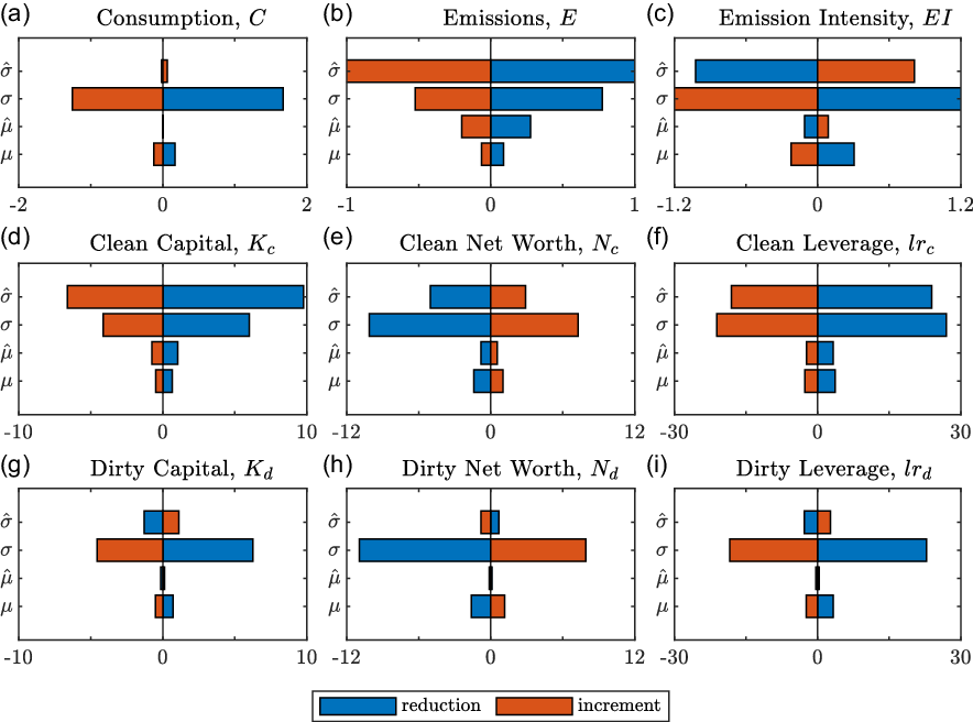
Figure 1 shows the sensitivity of key model variables in the steady state to changes in aggregate uncertainty
 $\sigma$
and aggregate bankruptcy cost
 $\mu$
as well as the degrees of asymmetry for both parameters,
 ${\mu _c}/{\mu _d}$
and
 ${\sigma _c}/{\sigma _d}$
. The equilibrium is moderately robust to changes in financial parameters. Figure 1 shows that macroeconomic variables (row 1) only slightly react. For instance, an increase of uncertainty
 $\sigma$
within both sectors by 25% reduces steady-state consumption by less than 2%. Sector-specific variables (rows 2 and 3) are however more sensitive. Financial variables (e.g. leverage, net worth) exhibit a higher sensitivity than nonfinancial variables (e.g. capital, labor (not shown)). All model variables exhibit a larger sensitivity to changes in uncertainty compared to changes in bankruptcy costs (
 $\sigma$
,
 ${\sigma _c}/{\sigma _d}$
vs.
 $\mu$
,
 ${\mu _c}/{\mu _d}$
). The steady state reacts more sensitively to reductions of parameter values than to increments. This suggests that the impact of frictions and asymmetries on the economy follows some concave functional relation, an observation that is reiterated in the dynamic sensitivity analysis in Section 4.2. In general, the clean sector is more sensitive to changes in financial asymmetries compared to the dirty sector (
 ${\sigma _c}/{\sigma _d}$
,
 ${\mu _c}/{\mu _d}$
, row 2 vs. row 3). This is intuitive. Following the definition of financial asymmetries from Section 3.2, a changing degree of asymmetry alters the financing conditions for the clean sector relative to the dirty sector. It directly impacts the clean sector’s competitiveness. However, due to the small size of the clean sector in the total economy, this has negligible ramifications for the dirty sector. Even if the market share of the clean sector doubles, dirty output would decline by less than 14%. For the dirty sector, the implications of changes to aggregate uncertainty and bankruptcy costs are much larger than the effects of changes to financial asymmetries (
 $\sigma$
and
 $\mu$
vs.
 ${\sigma _c}/{\sigma _d}$
and
 ${\mu _c}/{\mu _d}$
, row 3).
Steady-state sensitivity of sectoral variables with respect to key financial parameters bankruptcy cost
 $\mu$
, uncertainty
 $\sigma$
, and their asymmetric distribution among sectors
 $\mu _c/\mu _d$
and
 $\sigma _c/\sigma _d$
. Plots show the effect of increments (orange) and reductions (blue) of parameter values by 25%. Abscissas show the percentage change of variables in steady state.

In general, parameters that drive the degree of financial frictions and financial asymmetries have a small to modest influence on the equilibrium values especially for nonfinancial variables. This is intuitive because financial frictions matter for accumulation, adjustment, and transition dynamics such that given some disturbance, net worth positions adjust slower over time.
4. Simulations
In this section, we explore the interaction of climate policy with financial frictions and financial asymmetries. Specifically, we assess how frictions and asymmetries affect the sectoral responses to sudden increases of carbon pricing (permanent shock to emission tax
 $\tau _E$
), volatility in entrepreneurs’ financial wealth (temporary shock to net worth
 $N_{it}$
), and increased volatility in their idiosyncratic productivity (temporary shock to the standard deviation
 $\sigma _{it}$
of the productivity shock
 $\omega _{it}$
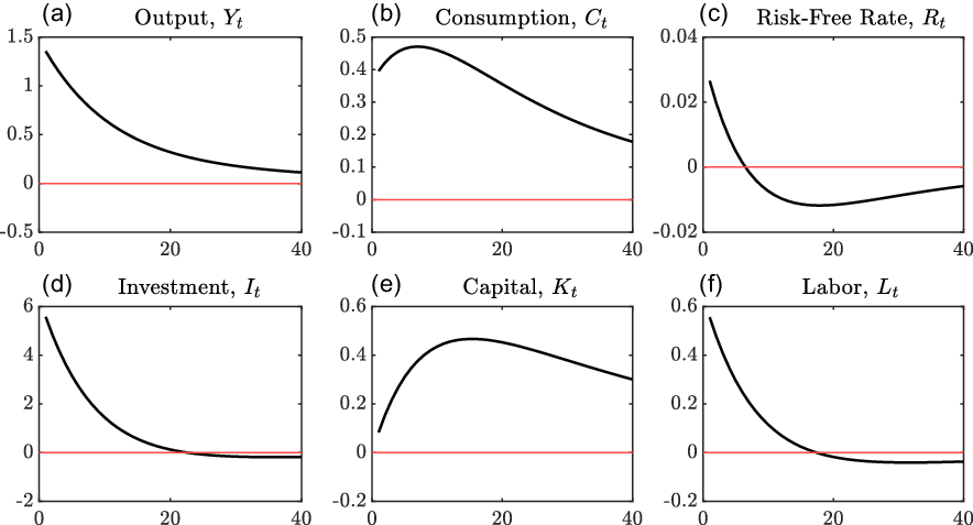
). But first, we start by simulating a standard productivity shock (modeled by temporary positive increase of total factor productivity) as it may occur from a breakthrough innovation to demonstrate the benchmark model dynamics in the absence of climate policy. Figure 2 shows impulse responses for key model variables.
Technology shock (1 SD) to the benchmark economy. Impulse response functions show quarterly percentage deviation from steady state. Graphs for investment and capital report aggregated responses.

The positive productivity shock has a direct, positive effect on output (panel (a)), fading over time. The initial increase in output is larger than the productivity shock (which is 1%) due to secondary effects. When total factor productivity rises, demands for labor and intermediate goods increase. Accordingly, wage rates and prices for intermediate goods and subsequently entrepreneurial returns increase (not shown). This lets entrepreneurs increase their borrowing thus exerting upward pressure on interest rates (c). Investment peaks (d) as entrepreneurs utilize the freshly acquired funds to expand capital stocks (e). Given the increased productivity, final goods producers will generate more output (a) until the shock fades and the economy returns to its steady state. Similar dynamics are found in many DSGE and E-DSGE models (cf. Christiano et al. (Reference Christiano, Motto and Rostagno2010); Annicchiarico and Di Dio (Reference Annicchiarico and Di Dio2015).
4.1 Transition dynamics
We now turn to the implication of financial frictions and financial asymmetries on the transition dynamics from a “dirty” to a “cleaner” economy. This transition is initiated by raising the carbon tax. We take as an exemplary scenario the ambition of the European Union 2030 Climate Target Plan: a reduction of domestic greenhouse gas emissions by at least 55% by 2030 compared to 1990. Relative to 2017 levels, that translates to a reduction by 45%.Footnote 19
Our research interest is whether and by how much frictions and asymmetries slow down and delay the transition and increase its cost in terms of lost consumption. We simulate the economy from 2017 to 2030, with a sudden, permanent emissions tax increment in 2017 calibrated to reduce emissions by 45% in 2030 in a counterfactual frictionless economy. We then study the behavior of our benchmark economy with financial frictions exposed to the same tax in order to identify the implications of inattention to frictions of policy makers when designing carbon taxes.
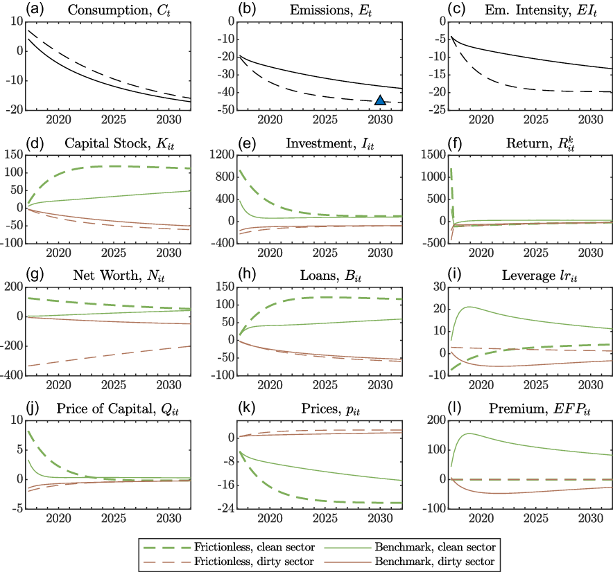
We find that financial frictions and financial asymmetries significantly delay the transition. More precisely, the EU will miss its 2030 climate target by approximately 11 percentage points if the implications of financial frictions are not considered when determining a carbon tax (Figure 3b). Instead of 55%, EU would only achieve emission reductions of 44% in 2030. If frictions were considered when determining the necessary tax rate to reach the climate target, the emissions tax implemented in 2017 would have to increase by 24% (Figure 5) to achieve the EU policy target. Delaying the implementation of climate policy to 2020 or even 2025 exacerbates both findings: the EU climate target is missed by 12 and 15 percentage points, respectively, and the necessary tax rates increase to 29% and 37%, respectively. We furthermore find that financial frictions generate financial transition risk in the clean sector which increases with the policy delay. In addition to its decelerating effects, frictions increase the social cost of the transition. We find that frictions can lead to a maximum reduction of per period consumption of approximately 4 percentage points.Footnote 20 Inertia and resulting costs are caused by the less pronounced redirection of investment flows between sectors and higher frictional losses.
Transition of the Euro Area economy from 2017 to 2030 under the impact of increased emission taxes. Graphs report percentage deviation relative to the 2017 economy. The triangle in panel (b) represents the 2030 climate target.

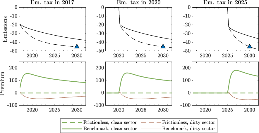
The effect of delayed climate policy. Graphs show percentage deviations from the economy in 2017. Column one is a reproduction from Figure 3. Columns two and three display the impact of an emissions tax implemented in 2020 and 2025, respectively. Triangles indicate the Euro Area 2030 climate target. In all three scenarios, the policy is not anticipated by agents.

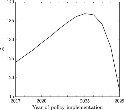
The ratio of required tax rates (benchmark economy to frictionless economy) subject to the year of policy implementation.

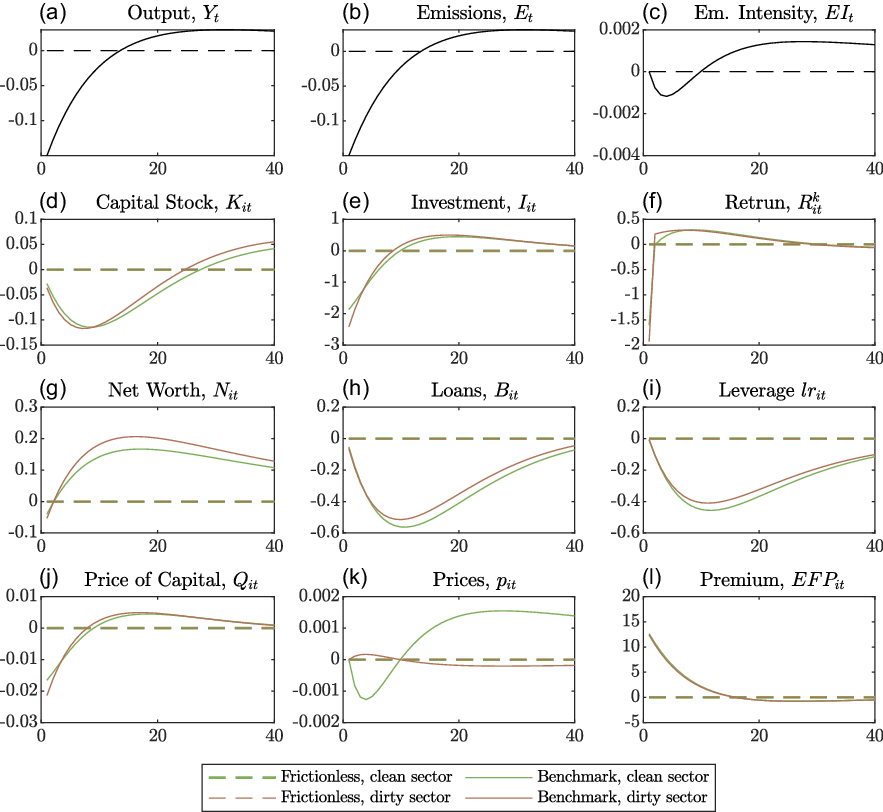
Figure 3 shows the effect of the increment in emissions taxes for benchmark and counterfactual scenarios. In 2017, a new emissions tax (approximately nine times the current tax level) is implemented. The counterfactual frictionless and the benchmark economy share the basic transmission mechanism of the permanent policy change: a higher emissions tax rate raises the marginal costs of production for the dirty sector, lowers the return on investment (f) and devalues dirty capital goods (j), which leads to corresponding adjustments in investment and capital stock (e, d), including divestment by capital goods producers (e), and consequently production of dirty goods is reduced. A loss of relative competitiveness of the dirty sector versus the clean sector exacerbates this effect. The clean sector expands production and gains market share. The clean sector’s relative competitive advantage caused by the higher emissions tax manifests in increasing prices of clean capital goods (j) and return on investment (f). Clean sector entrepreneurs adjust investment accordingly, financed primarily by increasing borrowing (h). As clean intermediate goods production grows, it crowds out dirty intermediate goods and changes the composition of the economy leading to lower emission intensities and lower per period emissions. Furthermore, carbon pricing triggers an immediate revaluation of entrepreneurial net worth
 $N_i$
(g). When the unexpected policy change hits the economy at the beginning of the period, returns on dirty investment decrease. However, entrepreneurs are stuck with the loans and capital stocks acquired during the previous period. With everything else fixed, the unexpected decline in profitability thus precipitates in a reduction of dirty net worth vice versa for the clean sector.
Even though the responses to the policy change is qualitatively similar for the frictionless and the benchmark economy, their quantitative implications are different. We first consider the frictionless economy (dashed and dotted lines in Figure 3) and then discuss major deviations in the benchmark economy. In the counterfactual frictionless economy, net worth positions adjust immediately and substantially after the policy change.Footnote 21 The absence of external finance premiums allows the clean sector to substantially expand borrowing, rapidly accumulate capital and scale up production. In the frictionless economy, investment adjustment costs are the only mechanism inhibiting an instant reallocation of capital from the dirty to the clean sector. The tax increment provides a sufficient steering effect to incentivize clean capital accumulation at scale such that the 2030 climate target is met.
When we account for financial frictions in the benchmark economy, the steering effect of the tax increment is dampened by frictional losses in addition to investment adjustment costs. With financial frictions, clean entrepreneurs increase investment (e) by less because borrowing is constrained by their net worth. In contrast to the frictionless economy, entrepreneurs have to build up sizable net worth positions (g) to limit the chance of bankruptcy and thus keep external finance premiums low. Entrepreneurs therefore maintain leverage ratios below 40% and utilize a combination of retained earnings and debt to finance their capital goods acquisitions. In the benchmark economy, the policy change causes a qualitatively similar immediate revaluation of net worth positions as in the frictionless economy, but on a smaller magnitude (approximately 5% more/less for clean/dirty entrepreneurs, barely visible in (g)). Net worth is accumulated through retained earnings from entrepreneurs with
 $\omega ^j_{it}\gt \bar{\omega }_{it}$
. This process requires time such that entrepreneurs rely on debt (h) when financing the scaling up of investment expenditures. Higher leverage (i) induces CMFs to charge higher premiums (l) to cover for the increased probability of bankruptcy. The higher premium reduces clean entrepreneurs’ ability to scale up investment (e), decelerates the accumulation of clean capital (d), and slows the transition (b).
Financial frictions slow the transition to such an extent that emissions in 2030 relative to 2017 are 9 percentage points above emissions in the frictionless scenario (b). Relative to 1990, emissions are 11 percentage points above the policy target in the friction economy. This implies that the European Union would miss its 2030 climate target, achieving emission reductions of approximately 44% instead of the envisaged 55%. Even though post-transition emissions of frictionless and benchmark economy eventually converge (not shown), cumulative emissions are higher in the delayed transition of the friction economy. Policy makers are well advised to consider the effect of financial frictions when designing climate policy, otherwise we see a risk that climate targets will not be met. Scenario analysis and climate policy assessments that include financial market frictions will therefore be particularly valuable to policy makers.
The precise impact of financial frictions on carbon budgets depends on their severity, the degree of financial asymmetry between the sectors, and the time available for the transition. In the following, we demonstrate how each of these criteria impacts transitional dynamics.
4.2 Policy delay, financial risk, and sensitivity
Time takes on a decisive role when debt is constrained by the borrowers’ net worth, which can only slowly be extended. With sufficient time, entrepreneurs could accumulate enough net worth to keep leverage ratios and external finance premiums low. Shortening the time horizon for the transition hence raises the relevance of financial frictions. If the implementation of climate policy is delayed and thus less time is available to realize the 2030 climate target, clean entrepreneurs have less time to increase their net worth positions through retained earnings. Therefore, they have to resort to debt financing to a greater extent. This further raises external finance premiums and limits the economic incentive for clean investment originating from the policy change. The transition is thus slowed down and emissions remain at higher levels for a longer transition period. Figure 4 visualizes the impact of delayed climate policy implementation on emissions and premiums. The first column of plots replicates the policy base case from the previous paragraph. Columns two and three show the response of the economy to a carbon tax increment implemented in 2020 and 2025, respectively. Tax rates are set such that the 2030 climate target is always met in the frictionless case. The gap in 2030 between the benchmark and the frictionless economy increases with the delay of the policy change. If implemented in 2017, frictions decelerate the response to the policy change such that emissions in 2030 are 9 percentage points higher compared to the frictionless economy. Delaying the policy change to 2020 and 2025 increases this difference to 10 and 12 percentage points, respectively. Translating the gap in emission reduction to the base year 1990 yields 11 percentage points for a policy change in 2017, and 12 and 15 percentage points for 2020 and 2025, respectively.
When the implementation of policy change is delayed, the carbon tax rates that provide the necessary steering effect have to be larger. Even in the frictionless scenario, the investment incentive from the tax must compensate for higher investment adjustment costs. In the benchmark economy, the tax has to compensate for larger frictional losses associated with a rapid transition in addition to higher investment adjustment costs. Due to the importance of retained earnings and net worth positions, the required compensation increases with the velocity of the transition.Footnote 22
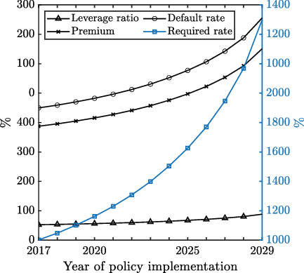
Figure 5 helps to disentangle the contribution of adjustment costs and frictional losses. We show the ratio of the required tax rates of the friction economy over the frictionless economy. If the policy change is implemented in 2017, the tax rate to reach the 2030 climate target in the friction economy is approximately 24% higher than the required rate in the frictionless economy. This divergence increases until 2025 where the required rate in the friction economy is approximately 37% higher. Any additional delay beyond 2025 causes required rates to converge. This is due to the fact that delaying the transition to the last years before 2030 alters the response of the economy fundamentally. Once the transition period is too short to restructure the economy and reallocate investment at scale and reasonable cost, it is less costly to achieve the reductions in emissions primarily by down-sizing the economy. In that case, no additional capital stock needs to be accumulated and frictions lose relevance. Hence, required tax rates for both scenarios converge.
Note that, in the benchmark economy, higher taxes increase financial transition risk in the clean sector. The more pressure policy makers apply to the economy, the larger the implications for leverage, default rates and risk premiums in the clean sector. At higher levels of the carbon tax, clean entrepreneurs find it profitable to finance investments through higher leverage ratios, pay larger premiums, and accept a higher likelihood of default. Figure 6 shows the response of the three financial indicators for clean entrepreneurs to the required tax rates (we show the maximum value across all time periods). When climate policy is implemented immediately (in 2017), the maximum values for leverage ratios, default rates, and risk premiums increase by 26%, 225%, and 194% relative to the pre-transition state. If climate policy is delayed until 2020 (but raised to the required rate), these values increase to 28%, 241%, and 208%, respectively. Implementing the required rate in 2025 implies maximum values of 34%, 289%, and 249%, respectively. The necessarily increased ambition in climate policy after a delay thus generates a “clean transition risk” for investments in the clean sector, which increases the social costs of the low-carbon transition due to higher default probabilities and hence a larger number of costly bankruptcies. Within the framework of our model, the default costs are fully recovered by financial intermediaries by charging a higher risk premium. However, policy makers may also be concerned about consequences of bankruptcy such as involuntary loss of employment and livelihood.
Required rates, leverage ratios, external finance premiums, and default rates for the benchmark economy. For the latter three financial indicators, only the maximum deviation from the pre-transition state is plotted (approx. 2 years after policy implementation).

Larger entrepreneurial leverage ratios undermine their capacity to cope well with business cycle dynamics or adverse shocks and might potentially endanger transition dynamics. With a clean sector that is vulnerable to financial transition risks, climate policy may benefit from sector specific policies to shield the clean sector, e.g. by derisking lending to the sector using instruments like loan guarantees (Steckel and Jakob (Reference Steckel and Jakob2018)). “Clean transition risk” also provides an additional reason to implement climate policy sooner rather than later, adding to the urgencies created, for example, by irreversibilities in climate change impacts, or by the limited feasible speed in rolling out new technologies.
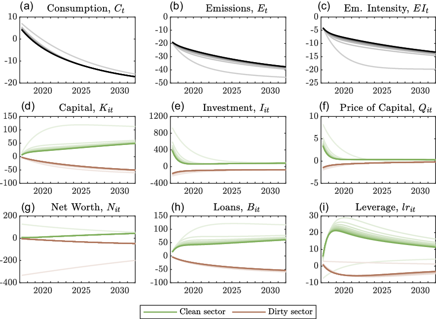
The speed of the transition triggered by a carbon price increase has turned out to be sensitive to financing conditions. Our base calibrations include two culprits that complicate financing the transition: first, the existence of financial frictions make any reallocation of capital involving external financing more costly. Second, financial asymmetries between the clean and dirty sector (in uncertainty and bankruptcy costs) generate relatively larger external finance premiums for the green sector. In this section, we disentangle the influence of these two (frictions and asymmetries) on the transition path of variables in a dynamic setting. For this, we vary both the degree of financial frictions and asymmetries. We find that the degree of financial frictions is a stronger determinant of transition dynamics. The counterfactual frictionless economy turns out to be an outlier. Even compared to the scenario with very small frictions, transition paths are substantially different. In line with the results from the static sensitivity analysis in Section 3.4, we find that the post-transition steady state equilibrium is robust to changes in frictions and asymmetries.
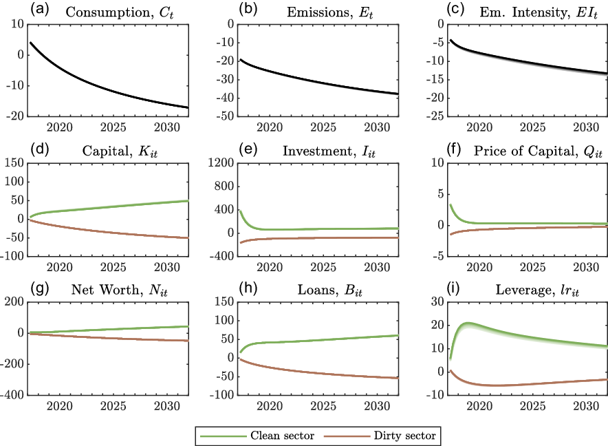
Figures 7 and 8 show parameter variations of financial frictions and financial asymmetries, respectively, where we reduce the degree of the frictions (
 $\mu$
) and the asymmetries (
 ${\mu _c}/{\mu _d}$
,
 ${\sigma _c}/{\sigma _d}$
) in steps of 10%. Paler shades of curves indicate lower frictions or less financial asymmetry. The frictionless economy (palest shade) is an extreme case in terms of invoked dynamics (Figure 7). Even a small increment in bankruptcy costs from 0 to
 $\mu =0.033$
(10% of the benchmark estimate from Table 1) dampens the intermediate effect of the emissions tax considerably reducing mitigation in 2030 by approximately 7 percentage points (b).Footnote
23
The strong reaction is caused by the fact that the slightest introduction of bankruptcy cost allocates an additional role to net worth such that it is not only used to finance capital internally but also limits the cost of external finance. Furthermore, time becomes an essential resource for entrepreneurs (net worth accumulation feeds from retained earnings) further stretching the transition period.
Sensitivity of the transition with respect to the degree of frictions in the economy. Graphs report percentage deviation relative to the 2017 economy where colors fade with decreasing
 $\mu \in [0,0.33]$
in steps of 10%. Darkest lines correspond to the benchmark calibration, whereas palest lines to the frictionless economy where
 $\mu =0$
.

Sensitivity of the transition with respect to the degree of financial asymmetry between sectors. Graphs report percentage deviation relative to the 2017 economy where colors fade with decreasing
 ${\mu _c}/{\mu _d}$
in steps of 10%. Darkest lines correspond to the benchmark calibration, whereas palest lines to the economy where
 ${\mu _c}/{\mu _d}=1$
.

Without financial asymmetries and in equilibrium (Figure 8), clean entrepreneurs maintain larger debt positions as compared to the benchmark economy. Their external finance premium is less sensitive towards leverage which makes the latter less costly. Therefore, given higher steady-state levels of leverage, the relative increment of debt (h) and leverage (i) in response to the policy change is less pronounced than in the benchmark economy. If financial asymmetries are eliminated, absolute increments however are more pronounced (not shown) such that dirty sector production is crowded out faster. The difference in emission reductions (b) between the benchmark economy and the economy without financial asymmetries amounts to 0.37 percentage points. Although the elimination of financial asymmetries increases the speed of the transition, their effect is of a different order of magnitude compared to the impact of frictions in general (Figure 7).
4.3 Temporary fluctuations
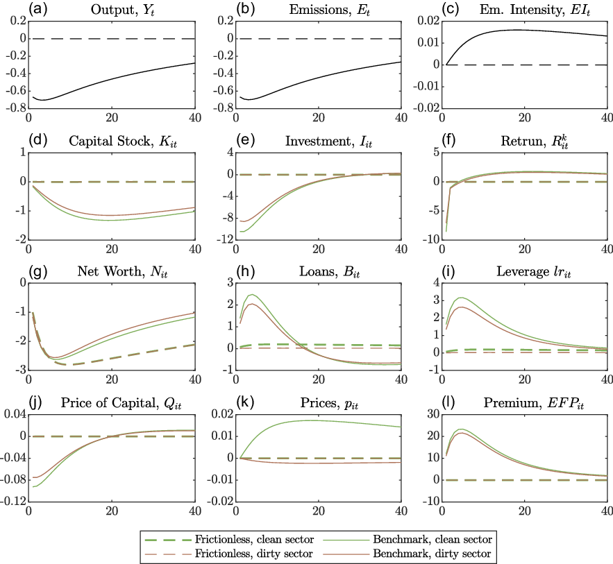
Sections 4.1 and 4.2 showed how the ability to borrow for entrepreneurs affects capital accumulation in climate policy scenarios. Macroeconomic fluctuations which affect financing conditions will thus affect capital accumulation in clean and dirty sector. In this section, we study the effect of short-run temporary disturbances on the performance of the clean and dirty sector. Specifically, we look at the dynamics generated by shocks to entrepreneurial net worth and uncertainty in the presence of financial frictions and asymmetries. We then show how the same shocks applied to both sectors affect clean and dirty sectors with different intensity thus altering their market shares (we use emission intensity as an indicator).
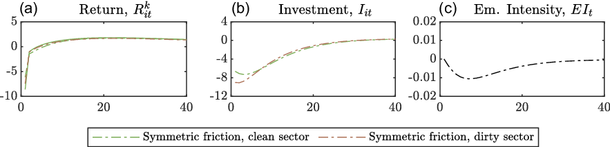
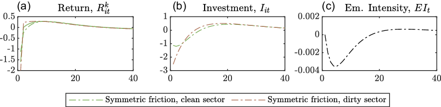
We attribute the different sectoral responses to their exposure to a risk effect and a volume effect. Both effects are rooted in the financial contract, which is sensitive to the financial frictions and financial characteristics of the lender. With respect to emission intensity, the consequences of the shocks depend on the susceptibility of the sectors to the effects as well as their relative strength.
The risk effect captures the change of the external finance premium with leverage. The strength of the risk effect is determined by the function
 $s_i(\!\cdot\!)$
in equation (12) which depends on uncertainty
 $\sigma _i$
and bankruptcy cost
 $\mu _i$
as parameters. Given a certain leverage, larger uncertainty
 $\sigma _i$
translates to a larger probability of default. Likewise, higher bankruptcy costs
 $\mu _i$
translate to a larger economic loss in case of default. Therefore, entrepreneurs that are subject to stronger financial frictions (via higher
 $\sigma _i$
and/or
 $\mu _i$
) face external finance premiums that are more sensitive to changes in leverage.
The volume effect is determined by the volume of the loan portfolio of an entrepreneur to which the external finance premium applies. As the external finance premium homogeneously applies to each unit of debt, changes in the premium have a stronger impact on entrepreneurs with larger volumes of debt outstanding.
In our setting, both effects partly counteract each other with respect to the distribution of sectoral market shares and hence emission intensity of the total economy. Due to the financial asymmetry in the benchmark calibration,
 $s'_c(\!\cdot\!)\gt s'_d(\!\cdot\!)$
and clean entrepreneurs are more susceptible to the risk effect. In equilibrium, the total debt volume of entrepreneurs in the dirty sector is more than eight times the volume of debt for clean sector entrepreneurs, making dirty entrepreneurs more susceptible to the volume effect.
We find that of the two shocks considered, the risk effect exhibits the larger persistence, and hence economically adverse shocks tilt the economy towards a higher emission intensity (Figures 9c and 11c). However, we do not find that these effects have a strong influence on the total emission intensity of the economy.
Financial wealth shock (1 SD). Impulse response functions show quarterly percentage deviation from steady state.

4.3.1 Financial wealth shock
As seen above, the role of entrepreneurial net worth positions and accumulation is crucial for the duration and cost of the transition. For publicly traded companies, their net worth is priced at exchanges through transactions between market participants. The valuation of net worth positions is thus subject to volatility induced by e.g. irrational behavior or imperfect information among traders. We study the impact of such volatility in the form of shocks to net worth positions to investigate if and how they impact clean sector performance and therefore the transition. Specifically, we consider a temporary negative and symmetric shock on clean and dirty entrepreneurial net worth positions. We show that such a financial wealth shock has strong implications for the economy. With financial asymmetries and thus risk and volume effects at work, sectoral responses are differentiated but the overall change in emission intensity is small.
We utilize impulse response function analysis to study the impact of a temporary symmetric negative shock
 $z_{Vt}$
of one standard deviation to entrepreneurial net worth positions in both sectors. Results in Figure 9 show how net worth positions decrease by 1% (g) upon impact and continue to decline as the shock fades. Since net worth positions are small and the shock is multiplicative, ramifications in the frictionless economy are negligible. The loss of up to 3% of net worth positions is compensated by slightly increasing debt (h) with infinitesimal effects on leverage.
In the friction economy, entrepreneurs substitute part of the foregone internal finance with debt (h) increasing their leverage ratios (i) at the cost of higher finance premiums (l) as CMFs will charge higher interest rates to cover for the increased bankruptcy probability. This in turn cripples prices of capital as well as entrepreneurial returns (j,f) and investment (e), producing lower capital stocks (d) and a contraction of output (a) and emissions (b). The financial wealth shock eliminates the same share of net worth from entrepreneurs in both sectors but the volume and risk effect produce differentiated sectoral responses. In our setting, the risk effect dominates the volume effect and the clean sector is at a disadvantage. Clean entrepreneurial returns and sector investment are reduced relatively more (e,f) creating a bias towards the dirty sector such that emission intensity (c) rises temporarily.
Figure 10 shows the response of the economy when both sectors exhibit identical financial characteristics and hence the risk effect impacts both sectors identically. Here, only the volume effect determines differentiated sectoral responses. Returns for dirty entrepreneurs decline more (f), slowing investment (e) and leading to a larger reduction in capital stock and the composition of the economy changes in favor of the clean sector. Comparing panels (c) in Figures 9 and 10, it becomes evident that the risk effect creates relatively more amplification and persistence in response to the financial wealth shock and compared to the volume effect. The magnitudes of changes to the composition of the economy and emission intensities are however small in both cases. The financial wealth shock that reduces net worth positions by 1% initially, increases the emission intensity of the economy by 0.02% at maximum (see panel (c) in Figure 9). Thus, a financial downturn simulated by a 10% negative financial wealth shock during the transition scenario from Section 4.1 does not alter transition dynamics substantially (not shown).
Financial wealth shock (1 SD) to an economy where financial asymmetries are eliminated. Impulse response functions show quarterly percentage deviation from steady state.

4.3.2 Uncertainty shock
We demonstrated in Sections 4.1 and 4.2 that the presence and strength of financial frictions can have a substantial influence on the performance of the clean sector during a transition. We further showed in Section 3.4 that, if frictions are present, changes to uncertainty
 $\sigma$
are a much stronger driver of results than changes to bankruptcy cost
 $\mu$
. This seems intuitive as uncertainty about idiosyncratic productivity shocks directly influence the risk associated with the profitability of entrepreneurs. Similar to Christiano et al. (Reference Christiano, Motto and Rostagno2014), who identify these uncertainty shocks (therein called “risk shocks”) as the most important shock driving business cycles, we introduced a disturbance
 $z_\sigma$
to the standard deviation
 $z_{\sigma t}\sigma _{it}$
of the productivity shock
 $\omega ^j_{it}$
. We confirm the finding from Section 4.3.1 that the risk effect exhibits a larger persistence, but this time the volume effects create larger amplification.
A shock to
 $z_{\sigma t}$
of one standard deviation temporarily increases the standard deviation
 $\sigma _{it}$
of the productivity shock
 $\omega _{it}$
and leads to higher uncertainty with respect to entrepreneurial profits and bankruptcies. The response of the economy is shown in Figure 11. Again, the shock has no impact on macroeconomic variables in the frictionless economy. A temporary increase in uncertainty is not a problem since bankruptcies are costless. In the benchmark economy however, increased uncertainty induces CMFs to ramp up external finance premiums (l) thereby diminishing returns to entrepreneurs (f) to which they react with deleveraging (i) and a contraction of investment (e). They accumulate net worth (g) to reduce individual premiums. As the shock fades and net worth positions have improved, after 10 quarters entrepreneurs start borrowing more from CMFs and leverage ratios converge back to the steady-state level. Together with relatively strong net worth positions, entrepreneurs temporarily invest above their steady state levels. Differentiated sector responses are again generated by the risk and volume effect.
Uncertainty shock (1 SD). Impulse response functions show quarterly percentage deviation from steady state.

In the beginning, the volume effect dominates: dirty entrepreneurs maintain larger debt positions and the contraction of dirty sector entrepreneurs’ return is more pronounced (f) as increasing risk premiums (l) apply to a larger loan volume. Dirty sector entrepreneurs sharply reduce expenditure for capital goods and divestment is more pronounced (e). During this time, clean entrepreneurs gain market share and emission intensity declines (c). As the volume effect fades, the dirty sector manages to retain a greater share of its earnings (g). This allows for a reduced contraction of borrowing compared to the clean sector’s response. After 10 quarters, the risk effect dominates. In comparison to the dirty sector, entrepreneurs in the clean sector have to cope with initially larger uncertainty
 $\sigma _c$
. An identical positive innovation to uncertainty exerts higher pressure on deleveraging (i) as leverage is more costly in terms of the external finance premium. The dirty sector gains market share and emission intensity temporarily exceeds the steady-state level as the risk effect outlasts the volume effect. Figure 12 shows impulse response functions for the risk shock in an economy that abstracts from financial asymmetries. The risk effect thus impacts sectors equally while the dirty sector remains more susceptible to the volume effect. Therefore, the clean sector occupies a market share above steady state throughout the shock horizon and the emission intensity is below its equilibrium value (c). The drop in emission intensity is twice that of Figure 11 and only a negligible overshoot materializes after period 20.
Uncertainty shock (1 SD) to an economy where financial asymmetries are eliminated. Impulse response functions show quarterly percentage deviation from steady state.

5. Conclusions
In this paper, we incorporate emissions and emission taxes in a DSGE model distinguishing clean and dirty production. We go beyond previous environmental DSGE models by incorporating sector-specific financial characteristics and financial frictions based on the financial accelerator mechanism (Bernanke et al. (Reference Bernanke, Gertler and Gilchrist1999)). The model is calibrated to the Euro Area utilizing company-level data for financial characteristics. We quantify the effect of financial frictions and asymmetric financial characteristics on the transition to a low-carbon economy initiated by increasing emission taxes. As an example, we model the ambition of the European Union 2030 Climate Target Plan. We furthermore study the impact of temporary shocks to entrepreneurial net worth and uncertainty on the performance of the clean and dirty sector.
We find that the tax rate necessary to achieve the 2030 climate target for the Euro Area is substantially higher when financial frictions are considered in the model (24% higher compared to the counterfactual frictionless economy). If policy makers do not account for the effect of financial frictions when setting the tax, emission reductions in 2030 fall 11 percentage points short of the EU’s target to reduce emissions by 55% relative to 1990.
We furthermore show that the adverse effects of financial frictions increase when climate policy is delayed and the transition needs to be accomplished more rapidly. For example, delaying the policy implementation to 2020 (or 2025), the gap in emission reductions relative to 1990 increases to 12 percentage points (or 15 percentage points, respectively). Keeping the announced 2030 climate target then requires tax rates that are 29% higher than the counterfactual (or 37% for the delay to 2025).
In the short term, financial frictions and asymmetries influence sector performance when the economy is hit by financial wealth shocks and uncertainty shocks. We trace differentiated sector responses to a risk and volume effect which impact sector performance differently. We find that adverse shocks decrease the competitiveness of the clean sector relatively stronger such that the dirty sector benefits from a larger market share during the shock horizon. Both effects have qualitative effects on the emission intensity of the economy but quantitative implications are small.
These findings suggest substantial consequences for policy design. Financial frictions undermine the impact of emission taxes, that, if designed for the counterfactual frictionless economy, will fail to steer the economy towards the envisaged climate targets. Therefore, financial markets need consideration in scenario analysis and integrated assessment modeling currently applied for policy making.
Climate change and mitigation are characterized by long time scales: inertia in the climate system, the slow process of innovation, irreversible tipping points, and technology lock-ins. This implies urgency to counteract climate change sooner rather than later. With financial frictions, we add another dimension to this list. The necessary reallocation of investment streams at reasonable costs is a slow process that is initiated as early as possible.
Our findings shed light on the effects of financial frictions on financial transition risk. The prospect of ambitious future climate policy puts “dirty” firms, which would be subject to this regulation, at risk (transition risk). When creditors internalize these risks, dirty firms face worse financing conditions for expanding or continuing their business. Financial transition risk, however, is also a risk for the competitiveness of “clean” firms whose profitability may be closely linked to climate policy. For a rapid transition, financial frictions generate high leverage ratios, large risk premiums, and high default rates in the clean sector. If the transition needs to be rushed, policy makers could consider additional policies to shield the clean sector and limit its vulnerability to shocks not associated with the transition.
Financing conditions are closely linked to climate policy: access to finance enables the private sector to respond to climate policy – but ambitious and rapid decarbonization creates risks that drive up financing costs. Our research takes first steps to endogenously consider the interaction of financing conditions and the policy-induced transition dynamics but more research is needed. For example, how can financial market policies flank climate policy to better cope with financial frictions. Furthermore, developing a modeling approach that combines financial frictions in the nonfinancial sector with frictions in the banking sector could shed light on impacts of interlinked financial market frictions on the steering effect of climate policy. Moreover, our approach focused on investment in the productive economy without explicit representation of research and development or technological learning. When these are modeled, frictions not only impact the accumulation of capital but also growth rates of sectoral factor productivity. This will then have further adverse effects on the transition. And finally, these features should be included in a modeling approach that allows for the realistic inclusion of damages (through stocks of carbon in the atmosphere not bound to steady states). This enables meaningful welfare analysis and an assessment of various policy mixes.
Acknowledgments
We would like to thank Beatriz Gaitan, Emilie Rosenlund Soysal, Francesca Diluiso, Boyan Yannovski, Ulrich Eydam, and Oliver Schenker for their insightful comments. Financial support by The German Federal Ministry of Education and Research (BMBF) provided as part of the FINFAIL project (grant 01LN1703A) is gratefully acknowledged.
A. Partial Correlation Analysis
Companies that innovate to reduce their carbon intensity or new entrants with innovative low-carbon technologies will often have substantial expenditures on research and development (Cole et al., Reference Cole, Elliott, Okubo and Zhou2013). The resulting intellectual properties are only partially reflected in these companies’ balance sheets. Therefore, we hypothesize that clean companies with less emission-intense businesses have relatively more intangible assets on their balance sheets than their emission-intense competitors. Balance sheets of the latter are expected to be composed of relatively more property, plant, and equipment (PP&E).
To test our hypotheses, we utilize company-level data from the database EIKON (Refinitiv (2020), data set equities) for 641 firms with headquarters in the Euro Area for the year 2019 and conduct two partial correlation analyses that determine the conditional correlation between the emission intensity of a company and, firstly, the ratio of PP&E to total assets and, secondly, the ratio of intangible assets to total assets. Emission intensity is calculated as estimated CO2 equivalents emission divided by total revenue. The ratio of PP&E to total assets is calculated as property/plant/equipment over total assets, and intangible assets to total assets arecalculated as intangibles over total assets.
We focus on the correlation of emission intensity and balance sheet composition for companies that are relatively similar with respect to their core business, i.e. companies belonging to the same sector. Otherwise, this exercise would be trivial as we would find that the emission intensity of a capital-intensive sector (e.g. aviation) is higher than for a labor-intensive sector (e.g. IT services). To eliminate the confounding effect of sector affiliation, we control for the association of firms according to The Refinitiv Business Classification framework (Refinitiv (2021)). The framework associates firms to 13 economics sectors (e.g. energy), 33 business sectors (e.g. fossil fuels), 62 industry groups (e.g. oil and gas), 154 industries (e.g. oil and gas exploration and production), and 898 activities (e.g. petroleum refining). The finer the definition of sectors, the stronger the control for the confounding effect of sector association, and the more alike the companies within a sector. For our analysis, we use firm association to either business sector, industry group, or industry as control variable.
Table A1 presents the Spearman’s rank correlation coefficients for both partial correlation analyses. In line with our hypothesis, we find very strong evidence for a positive correlation between a firm’s emission intensity and its share of PP&E in total assets. For a negative correlation between emission intensity and its share of intangible assets in total assets, we find very strong evidence in models 1 and 2. Significance levels decrease with increasing specificity of the control variable as less firms remain in the clustered subsets of the data. Correlation coefficients decrease with increasing specificity of the control variable (i.e. sector definitions move from coarse to fine), suggesting that sectoral association explains part of the correlation. But even when controlling for sector association at the industry level (model 4), some degree of significant association remains. These results are robust when controlling for the location (country) of the firm’s headquarters in addition to sector association (not reported).
Partial correlation analysis

Significance: *** p < 0.01, ** p < 0.05, * p < 0.1. Fossil and renewable energy sectors are aggregated into one business sector energy. For all respective firms, industry groups and industry associations are energy.
B. Derivation of the Optimal Financial Contract
This section is in principle a brief summary of one of the appendices in Bernanke et al. (Reference Bernanke, Gertler and Gilchrist1999) and will provide the derivation of the financial contract. The financial contract offered by CMFs to entrepreneurs is a contingent standard debt contract which maximizes entrepreneurial returns subject to the perfectly competitive CMF’s zero-profit condition.
 \begin{equation*} \max _{\left \{ l_{it+1}^{j}\right \},\left \{ \bar {\omega }_{it+1}^{j}\right \} }E_{t}\left \{ R_{it+1}^{k}l_{it+1}^{j}N_{it+1}^{j}\left [ 1-\Gamma \left ( \bar {\omega }_{it+1}^{j}\right ) \right ] \right \} \end{equation*}
 \begin{equation*} \textbf {s.t. }\left [ \Gamma \left ( \bar {\omega }_{it+1}^{j}\right ) -\mu _{i}G\left ( \bar {\omega }_{it+1}^{j}\right ) \right ] R_{it+1}^{k}l_{it+1}^{j}N_{it+1}^{j}= R_{t+1}\left ( l_{it+1}^{j}-1\right ) N_{it+1}^{j} \end{equation*}
Due to constant returns to scale production technologies, the maximization problem can be normalized by net worth yielding the following Lagrangian:
 \begin{align*} L &= E_{t}\left \{ R_{it+1}^{k}l_{it+1}^{j}\left[ 1-\Gamma \left ( \bar {\omega }_{it+1}^{j}\right ) \right] +\lambda _{it}^{j}\left ( \left [ \Gamma \left ( \bar {\omega }_{it+1}^{j}\right ) -\mu _{i}G\left ( \bar {\omega }_{it+1}^{j}\right ) \right ] R_{it+1}^{k}l_{it+1}^{j}\right.\right. \\& \quad - \left.\left. \left ( 1+\tau _{it}^{B}\right ) R_{t+1}\left ( l_{it+1}^{j}-1\right ) \right ) \right \} \end{align*}
with first-order conditions
 \begin{align} l_{it+1}^{j}\;:\;0& =R_{it+1}^{k}\left [ 1-\Gamma \left ( \bar{\omega }_{it+1}^{j}\right ) \right ] +\lambda _{it}^{j}\left ( \left [ \Gamma \left ( \bar{\omega }_{it+1}^{j}\right ) -\mu _{i}G\left ( \bar{\omega }_{it+1}^{j}\right ) \right ] R_{it+1}^{k}- R_{t+1}\right ) \nonumber \\[5pt] 0 &=\frac{R_{it+1}^{k}}{ R_{t+1}}\left [ 1-\Gamma \left ( \bar{\omega }_{it+1}^{j}\right ) \right ] +\lambda _{it}^{j}\left ( \left [ \Gamma \left ( \bar{\omega }_{it+1}^{j}\right ) -\mu _{i}G\left ( \bar{\omega }_{it+1}^{j}\right ) \right ] \frac{R_{it+1}^{k}}{R_{t+1}}-1\right ) \end{align}
 \begin{align} \frac{R_{it+1}^{k}}{ R_{t+1}} =\frac{\lambda _{it}^{j}}{\left [ 1-\Gamma \left ( \bar{\omega }_{it+1}^{j}\right ) \right ] +\lambda _{it}^{j}\left [ \Gamma \left ( \bar{\omega }_{it+1}^{j}\right ) -\mu _{i}G\left ( \bar{\omega }_{it+1}^{j}\right ) \right ] } \end{align}
 \begin{align} \bar{\omega }_{it+1}^{j}\;:\;0 & =R_{it+1}^{k}l_{it+1}^{j}\left [ -\Gamma ^{\prime }\left ( \bar{\omega }_{it+1}^{j}\right ) \right ] +\lambda _{it}^{j}\left ( \left [ \Gamma ^{\prime }\left ( \bar{\omega }_{it+1}^{j}\right ) -\mu _{i}G^{\prime }\left ( \bar{\omega }_{it+1}^{j}\right ) \right ] R_{it+1}^{k}l_{it+1}^{j}\right ) \nonumber \\[5pt] \lambda _{it}^{j} &=\frac{\Gamma ^{\prime }\left ( \bar{\omega }_{it+1}^{j}\right ) }{\Gamma ^{\prime }\left ( \bar{\omega }_{it+1}^{j}\right ) -\mu _{i}G^{\prime }\left ( \bar{\omega }_{it+1}^{j}\right ) } \nonumber \\[5pt] \lambda _{it}^{j}\;:\;0&= R_{t+1}\left ( l_{it+1}^{j}-1\right ) -\left [ \Gamma \left ( \bar{\omega }_{it+1}^{j}\right ) -\mu _{i}G\left ( \bar{\omega }_{it+1}^{j}\right ) \right ] R_{it+1}^{k}l_{it+1}^{j} \end{align}
The term
 $\frac{R_{it+1}^{k}}{ R_{t+1}}$
in equation (18) describes the return a unit of capital has to generate discounted by taxes and the interest rate demanded by households. In above one, it can be thought of as a premium the capital stock has to generate due to the external finance obtained. In their appendix A, Bernanke et al. (Reference Bernanke, Gertler and Gilchrist1999) show that there is an interior solution to this optimization problem and that
 $\lambda _{it}^{j}$
is monotonically increasing in
 $\bar{\omega }_{it+1}^{j}$
and that
 $\frac{R_{it+1}^{k}}{ R_{t+1}}$
is monotonically increasing in
 $\lambda _{it}^{j}$
and thus also
 $\bar{\omega }_{it+1}^{j}$
. Equation (18) therefore shows the monotonically increasing relationship between default probabilities expressed via the cutoff productivity and the premium on external funds. Define
 \begin{equation*} \rho \left ( \bar {\omega }_{it+1}^{j}\right ) =\frac {\lambda _{it}^{j}}{\left ( 1-\Gamma \left ( \bar {\omega }_{it+1}^{j}\right ) \right ) +\lambda _{it}^{j}\left [ \Gamma \left ( \bar {\omega }_{it+1}^{j}\right ) -\mu _{i}G\left ( \bar {\omega }_{it+1}^{j}\right ) \right ] } \end{equation*}
such that
 \begin{equation*} \frac {R_{it+1}^{k}}{ R_{t+1}}=\rho \left ( \bar {\omega }_{it+1}^{j}\right ) \end{equation*}
inverting this expression yields
 \begin{equation*} \bar {\omega }_{it+1}^{j}= {\bar {\boldsymbol\omega }}_{i}\left ( \frac {R_{it+1}^{k}}{R_{t+1}}\right ) \end{equation*}
Since
 $R_{t+1}$
and
 $\tau _{it}^{B}$
apply to all entrepreneurs within a sector and it was shown in the text that entrepreneurs within a sector
 $i$
will have identical
 $R_{it+1}^{k}$
,
 $\bar{\omega }_{it+1}^{j}$
is determined through aggregates only. Therefore, it must be identical across entrepreneurs within a sector and equal to
 $\bar{\omega }_{it+1}$
. Rearranging (20) for leverage and acknowledging that cutoff productivities will be identical across sector
 $i$
entrepreneurs yields
 \begin{eqnarray*} l_{it+1}^{j} &=&\frac{1}{1-\left [ \Gamma \left ( \bar{\omega }_{it+1}\right ) -\mu _{i}G\left ( \bar{\omega }_{it+1}\right ) \right ] \frac{R_{it+1}^{k}}{R_{t+1}}} \\[5pt] &=&\frac{1}{1-\left [ \Gamma \left ( \bar{\omega }_{it+1}\right ) -\mu _{i}G\left ( \bar{\omega }_{it+1}\right ) \right ] \rho \left ( \bar{\omega }_{it+1}\right ) }=\Psi _{i}\left ( \bar{\omega }_{it+1}\right ) \end{eqnarray*}
proving that also leverage will be identical for all entrepreneurs within sector
 $i$
and equal to
 $l_{it+1}$
. Appendix A in Bernanke et al. (Reference Bernanke, Gertler and Gilchrist1999) shows that
 $\Psi _{i} ( \bar{\omega }_{it+1} )$
is monotonically increasing in
 $\bar{\omega }_{it+1}$
and we have
 \begin{equation*} l_{it+1}=\Psi _{i}\left ( \bar {\omega }_{it+1}\right ) =\Psi _{i}\left ( {\bar {\boldsymbol\omega }}_{i}\left ( \frac {R_{it+1}^{k}}{ R_{t+1}}\right ) \right ) =\psi _{i}\left ( \frac {R_{it+1}^{k}}{\left ( 1+\tau _{it}^{B}\right ) R_{t+1}}\right ) \end{equation*}
where also
 $\psi _{i}$
is monotonically increasing in
 $\bar{\omega }_{it+1}$
. Now substitute (6) to arrive at
 \begin{equation*} Q_{it}K_{it+1}^{j}=\psi _{i}\left ( \frac {R_{it+1}^{k}}{\left ( 1+\tau _{it}^{B}\right ) R_{t+1}}\right ) N_{it+1}^{j} \end{equation*}
This equation shows the proportionality of capital expenditures to net worth with the factor of proportionality increasing with expected return to capital. As Bernanke et al. (Reference Bernanke, Gertler and Gilchrist1999) note that, ceteris paribus, a rise in the expected return to capital reduces the expected default probability which allows the entrepreneur to extend borrowing and the size of his business. Along the process, rising leverage implies increasing default probabilities which constrain the entrepreneur from borrowing infinite amounts. Invert above expression to arrive at
 \begin{equation*} R_{it+1}^{k}=s_i\left ( l_{it+1}\right ) R_{t+1} \end{equation*}
with
 $s_i^{\prime } ( l_{it+1} ) \gt 0.$
This equation describes the connection between the leverage ratio of an entrepreneur and the required rate of return on capital. Combining equations (18) and (20) and eliminating the index for individual entrepreneurs from leverage and cutoff productivity yields
 \begin{equation*} 0=\frac {R_{it+1}^{k}}{ R_{t+1}}\left [ 1-\Gamma \left ( \bar {\omega }_{it+1}\right ) \right ] +\frac {\Gamma ^{\prime }\left ( \bar {\omega }_{it+1}\right ) }{\Gamma ^{\prime }\left ( \bar {\omega }_{it+1}\right ) -\mu _{i}G^{\prime }\left ( \bar {\omega }_{it+1}\right ) }\left ( \left [ \Gamma \left ( \bar {\omega }_{it+1}\right ) -\mu _{i}G\left ( \bar {\omega }_{it+1}\right ) \right ] \frac {R_{it+1}^{k}}{ R_{t+1}}-1\right ) \end{equation*}
that, together with the constraint
 \begin{equation*} 0=\left [ \Gamma \left ( \bar {\omega }_{it+1}\right ) -\mu _{i}G\left ( \bar {\omega }_{it+1}\right ) \right ] R_{it+1}^{k}l_{it+1}-R_{t+1}\left ( l_{it+1}-1\right ) \end{equation*}
characterizes the financial contract offered to entrepreneur
 $j$
in sector
 $i.$
C. Derivation of Aggregate Sectoral Net Worth
If the density of entrepreneurs with net worth
 $N_{it+1}^{j}$
is denoted by
 $f ( N_{it+1}^{j} )$
then the aggregate average net worth for entrepreneurs in group
 $i$
is
 $N_{it+1}=\int _{N_{it+1}^{j}}N_{it+1}^{j}f ( N_{it+1}^{j} ) dN_{it+1}^{j}$
. In period
 $t$
, after selling depreciated capital to capital goods producers, settling debt, and paying taxes, entrepreneur
 $j$
is left with (equation 6).
 \begin{eqnarray*} V_{it}^{j} &=&z_{Vt}R_{it}^{k}l_{it}^{j}N_{it}^{j}\left [ 1-\Gamma \left ( \bar{\omega }_{it}^{j}\right ) \right ] \\[5pt] V_{it}^{j} &=&z_{Vt}R_{it}^{k}Q_{it-1}K_{it}^{j}\left [ 1-\Gamma \left ( \bar{\omega }_{it}^{j}\right ) \right ] \end{eqnarray*}
Note that due to the character of the optimal financial contract, leverage and cutoff productivity are independent of entrepreneurial net worth, we can thus eliminate the superscript
 $j$
from
 $\bar{\omega }_{it}^{j}$
and
 $l_{it}^{j}$
with
 $l_{i,t}=\frac{Q_{it-1}K_{it}}{N_{it}}$
where
 $K_{it}=\int _{N_{it}^{j}}K_{it}^{j}f ( N_{it}^{j} ) dN_{it}^{j}$
. Multiplying (6) by
 $f ( N_{i,t}^{j} )$
and integrating over entrepreneurs belonging to group
 $i$
yields
 \begin{eqnarray} V_{it} &=&\int _{N_{it}^{j}}V_{it}^{j}f\left ( N_{it}^{j}\right ) dN_{it}^{j} \nonumber \\[5pt] &=&\int _{N_{it}^{j}}z_{Vt}R_{it}^{k}l_{it}N_{it}^{j}\left [ 1-\Gamma \left ( \bar{\omega }_{it}\right ) \right ] f\left ( N_{it}^{j}\right ) dN_{it}^{j} \nonumber \\[5pt] &=&z_{Vt}R_{it}^{k}l_{it}N_{it}\left [ 1-\Gamma \left ( \bar{\omega }_{it}\right ) \right ] \nonumber \\[5pt] &=&z_{Vt}\left ( R_{it}^{k}l_{it}N_{it}-\left [ \Gamma \left ( \bar{\omega }_{it}\right ) -\mu _{i}G\left ( \bar{\omega }_{it}\right ) +\mu _{i}G\left ( \bar{\omega }_{it}\right ) \right ] R_{it}^{k}l_{it}N_{it}\right ) \nonumber \\[5pt] &=&z_{Vt}\left ( R_{it}^{k}l_{it}N_{it}-\left [ \Gamma \left ( \bar{\omega }_{it}\right ) -\mu _{i}G\left ( \bar{\omega }_{it}\right ) \right ] R_{it}^{k}l_{it}N_{it}-\mu _{i}G\left ( \bar{\omega }_{it}\right ) R_{it}^{k}l_{it}N_{it}\right ) \end{eqnarray}
We can aggregate the zero-profit condition of CMFs (equation 9) by multiplying both sides by
 $f ( N_{i,t}^{j} )$
and integrating over entrepreneurs which gives
 \begin{equation*} \left [ \Gamma \left ( \bar {\omega }_{it}\right ) -\mu _{i}G\left ( \bar {\omega }_{it}\right ) \right ] R_{it}^{k}l_{it}N_{it}= R_{t+1}\left ( l_{it}-1\right ) N_{it} \end{equation*}
and can be substituted into equation (21) to yield
 \begin{eqnarray*} V_{it} &=&z_{Vt}\left ( R_{it}^{k}l_{it}N_{it}- R_{t+1}\left ( l_{it}-1\right ) N_{it}-\mu _{i}G\left ( \bar{\omega }_{it}\right ) R_{it}^{k}l_{it}N_{it}\right ) \\[5pt] &=&z_{Vt}\left ( R_{it}^{k}l_{it}N_{it}-\left \{ \left ( 1+\tau _{it}^{B}\right ) R_{t+1}+\frac{\mu _{i}G\left ( \bar{\omega }_{it}\right ) R_{it}^{k}l_{it}N_{it}}{\left ( l_{it}-1\right ) N_{it}}\right \} \left ( l_{it}-1\right ) N_{it}\right ) \\[5pt] &=&z_{Vt}\left ( R_{it}^{k}Q_{it-1}K_{it}-\left \{ \left ( 1+\tau _{it}^{B}\right ) R_{t+1}+\frac{\mu _{i}G\left ( \bar{\omega }_{it}\right ) R_{it}^{k}Q_{it-1}K_{it}}{Q_{it-1}K_{it}-N_{it}}\right \} \left ( Q_{it-1}K_{it}-N_{it}\right ) \right ) \end{eqnarray*}
where the second term in brackets is expected default costs over loans and corresponds to the external finance premium. A fraction of entrepreneurs will close down their businesses with probability
 $1-\nu _{i}$
, and the fraction
 $\nu _{i}$
will continue operating their businesses. This model follows Christiano et al. (Reference Christiano, Motto and Rostagno2014) and Gertler and Karadi (Reference Gertler and Karadi2011) with the large family assumption. When exiting the economy, entrepreneurs transfer their wealth to households who, each period, transfer part of their wealth
 $M_{i}$
to entrepreneurs. This assumptions prevent entrepreneurs to be fully self-financed and also guarantee positive net worth for all entrepreneurs. The average net worth of entrepreneurs after exit, entry, and transfers realized corresponds to
 \begin{eqnarray} N_{it+1} &=&\nu _{t}V_{it}+M_{i} \nonumber \\[5pt] N_{it+1} &=&\nu _{t}z_{Vt}\left ( R_{it}^{k}Q_{it-1}K_{it}-\left \{ \left ( 1+\tau _{it}^{B}\right ) R_{t+1}+\frac{\mu _{i}G\left ( \bar{\omega }_{it}\right ) R_{it}^{k}Q_{it-1}K_{it}}{Q_{it-1}K_{it}-N_{it}}\right \} \left ( Q_{it-1}K_{it}-N_{it}\right ) \right ) +M_{i} \nonumber \\&& \end{eqnarray}
D. Translation into Dynare Code
This appendix will derive the Dynare code for the equations where it is not trivial, i.e. the financial contract.
 \begin{eqnarray*} 0 &=&\frac{R_{it+1}^{k}}{ R_{t+1}}\left [ 1-\Gamma \left ( \bar{\omega }_{it+1}\right ) \right ] +\frac{\Gamma ^{\prime }\left ( \bar{\omega }_{it+1}\right ) }{\Gamma ^{\prime }\left ( \bar{\omega }_{it+1}\right ) -\mu _{i}G^{\prime }\left ( \bar{\omega }_{it+1}\right ) }\left ( \left [ \Gamma \left ( \bar{\omega }_{it+1}\right ) -\mu _{i}G\left ( \bar{\omega }_{it+1}\right ) \right ] \frac{R_{it+1}^{k}}{ R_{t+1}}-1\right ) \\[5pt] 0 &=&\left [ \Gamma \left ( \bar{\omega }_{it+1}\right ) -\mu _{i}G\left ( \bar{\omega }_{it+1}\right ) \right ] R_{it+1}^{k}l_{it+1}N_{it+1}-\left ( 1+\tau _{it}^{B}\right ) R_{t+1}\left ( l_{it+1}-1\right ) N_{it+1} \end{eqnarray*}
with
 \begin{eqnarray*} \Gamma \left ( \bar{\omega }_{it+1}\right ) &=&\bar{\omega }_{it+1}\left [ 1-F\left ( \bar{\omega }_{it+1}\right ) \right ] +G\left ( \bar{\omega }_{it+1}\right ) \\[5pt] G\left ( \bar{\omega }_{it+1}\right ) &=&\int _{0}^{\bar{\omega }_{it+1}}\omega _{it+1}dF\left ( \omega _{it+1}\right ) \end{eqnarray*}
The derivatives can be expressed as follows:
 \begin{eqnarray*} G\left ( \bar{\omega }_{it+1}\right ) &=&\int _{0}^{\bar{\omega }_{it+1}}\omega _{it+1}dF\left ( \omega _{it+1}\right ) =\int _{0}^{\bar{\omega }_{it+1}}\omega _{it+1}f\left ( \omega _{it+1}\right ) d\omega _{it+1} \\[5pt] G^{\prime }\left ( \bar{\omega }_{it+1}\right ) &=&\frac{d}{d\bar{\omega }_{it+1}}\int _{0}^{\bar{\omega }_{it+1}}\omega _{it+1}f\left ( \omega _{it+1}\right ) d\omega _{it+1} \\[5pt] &=&\bar{\omega }_{it+1}f\left ( \bar{\omega }_{it+1}\right ) \end{eqnarray*}
and
 \begin{eqnarray*} \Gamma \left ( \bar{\omega }_{it+1}\right ) &=&\int _{0}^{\bar{\omega }_{it+1}}\omega _{it+1}dF\left ( \omega _{it+1}\right ) +\bar{\omega }_{it+1}\left [ 1-F\left ( \bar{\omega }_{it+1}\right ) \right ] \\[5pt] \Gamma ^{\prime }\left ( \bar{\omega }_{it+1}\right ) &=&\bar{\omega }_{it+1}f\left ( \bar{\omega }_{it+1}\right ) +\left [ 1-F\left ( \bar{\omega }_{it+1}\right ) \right ] -\bar{\omega }_{it+1}f\left ( \bar{\omega }_{it+1}\right ) \\[5pt] &=&\left [ 1-F\left ( \bar{\omega }_{it+1}\right ) \right ] \end{eqnarray*}
Now, we need to find expressions for
 $F ( \bar{\omega }_{it+1} )$
,
 $G ( \bar{\omega }_{it+1} )$
and
 $f ( \bar{\omega }_{it+1} )$
. Dynare cannot handle lognormal distributions, so we transform them in order to express them in terms of the probability density function and cumulative distribution function of the standard normal distribution. In order to ease readability of the following deviation, we shall omit the time and the sector indices. We will start with the dynare input for
 $F ( \bar{\omega } )$
. The probability density function and cumulative distribution function are denoted by
 $f ( \omega )$
and
 $F ( \omega )$
for lognormally distributed
 $\omega$
.
 \begin{equation*} F\left ( \bar {\omega }\right ) =\int _{0}^{\bar {\omega }}f\left ( \omega \right ) d\omega \end{equation*}
Now substitute
 \begin{eqnarray*} \omega &=&e^{x}=\gt x=\log \omega \sim N\left ( \mu _{x},\sigma _{x}^{2}\right ) \\[5pt] &=&\gt \frac{d\omega }{dx}=e^{x}=\gt d\omega =e^{x}dx \end{eqnarray*}
Since
 $\omega$
is lognormally distributed,
 $x=\log ( \omega )$
is normally distributed, i.e.
 $e^{x}$
is lognormally distributed and
 $f$
is the normal density function. Adjust boundaries knowing that
 $x=\log \omega$
so
 $\bar{\omega }\rightarrow \log ( \bar{\omega } )$
and
 $0\rightarrow -\infty$
 \begin{eqnarray*} F\left ( \bar{\omega }\right ) &=&\int _{0}^{\bar{\omega }}f\left ( \omega \right ) d\omega =\int _{-\infty }^{\log \bar{\omega }}f\left ( e^{x}\right ) e^{x}dx \\[5pt] &=&\int _{-\infty }^{\log \bar{\omega }}\frac{1}{e^{x}\sigma _{x}\sqrt{2\pi }}e^{-\frac{\left ( \ln e^{x}-Ex\right ) ^{2}}{2\sigma _{x}^{2}}}e^{x}dx \\[5pt] &=&\frac{1}{\sigma _{x}\sqrt{2\pi }}\int _{-\infty }^{\log \bar{\omega }}e^{-\frac{\left ( x-Ex\right ) ^{2}}{2\sigma _{x}^{2}}}dx \end{eqnarray*}
where
 \begin{eqnarray*} Ee^{x} &=&E\omega =1 \\[5pt] 1 &=&Ee^{x}=e^{\left [ Ex+\frac{\sigma _{x}^{2}}{2}\right ] } \\[5pt] &=&\gt Ex=-\frac{\sigma _{x}^{2}}{2} \end{eqnarray*}
so
 \begin{eqnarray*} \int _{0}^{\bar{\omega }}f\left ( \omega \right ) d\omega &=&\frac{1}{\sigma _{x}\sqrt{2\pi }}\int _{-\infty }^{\log \bar{\omega }}e^{-\frac{\left ( x-Ex\right ) ^{2}}{2\sigma _{x}^{2}}}dx \\[5pt] &=&\frac{1}{\sigma _{x}\sqrt{2\pi }}\int _{-\infty }^{\log \bar{\omega }}e^{-\frac{1}{2}\left ( \frac{x+\frac{\sigma _{x}^{2}}{2}}{\sigma _{x}}\right ) ^{2}}dx \end{eqnarray*}
Now substitute
 \begin{eqnarray*} \frac{x+\frac{\sigma _{x}^{2}}{2}}{\sigma _{x}} &=&v \\[5pt] &=&\gt \frac{dv}{dx}=\frac{1}{\sigma _{x}}=\gt dx=\sigma _{x}dv \end{eqnarray*}
Recall that
 $x$
is normally distributed, so is
 $v$
. Adjust boundaries knowing that
 $v=\frac{x+\frac{\sigma _{x}^{2}}{2}}{\sigma _{x}}$
so
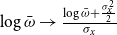 $\log \bar{\omega }\rightarrow \frac{\log \bar{\omega }+\frac{\sigma _{x}^{2}}{2}}{\sigma _{x}}$
and
 $-\infty \rightarrow -\infty$
 \begin{eqnarray*} \int _{0}^{\bar{\omega }}f\left ( \omega \right ) d\omega &=&\frac{1}{\sigma _{x}\sqrt{2\pi }}\int _{-\infty }^{\frac{\log \bar{\omega }+\frac{\sigma _{x}^{2}}{2}}{\sigma _{x}}}e^{-\frac{v^{2}}{2}}\sigma _{x}dv \\[5pt] F\left ( \bar{\omega }\right ) &=&\int _{0}^{\bar{\omega }}f\left ( \omega \right ) d\omega =\text{prob}\left [ \log \omega \leq \frac{\log \bar{\omega }+\frac{\sigma _{x}^{2}}{2}}{\sigma _{x}}\right ] \end{eqnarray*}
For the Dynare code, the following expression can thus be utilized
 \begin{equation} F\left ( \bar{\omega }\right ) =normcdf\left [ \frac{\log \bar{\omega }+\frac{\sigma _{x}^{2}}{2}}{\sigma _{x}}\right ] \end{equation}
Next, we derive the Dynare expression for
 $G ( \bar{\omega } ) .$
The probability density function and cumulative distribution function are denoted by
 $f ( \omega )$
and
 $F ( \omega )$
for lognormally distributed
 $\omega$
.
 \begin{equation*} G\left ( \bar {\omega }\right ) =\int _{0}^{\bar {\omega }}\omega dF\left ( \omega \right ) =\int _{0}^{\bar {\omega }}\omega f\left ( \omega \right ) d\omega \end{equation*}
Now substitute
 \begin{eqnarray*} \omega &=&e^{x}\rightarrow x=\ln \omega \sim N\left ( \mu _{\ln x},\sigma _{\ln x}^{2}\right ) \\[5pt] &\rightarrow &\frac{d\omega }{dx}=e^{x}\rightarrow d\omega =e^{x}dx \end{eqnarray*}
Since
 $\omega$
is lognormally distributed, i.e.
 $x=\log ( \omega )$
is normally distributed, i.e.
 $e^{x}$
is lognormally distributed. Adjust boundaries knowing that
 $x=\log \omega$
so
 $\bar{\omega }\rightarrow \log ( \bar{\omega } )$
and
 $0\rightarrow -\infty$
 \begin{eqnarray*} G\left ( \bar{\omega }\right ) &=&\int _{0}^{\bar{\omega }}\omega dF\left ( \omega \right ) =\int _{-\infty }^{\log \bar{\omega }}e^{x}f\left ( e^{x}\right ) e^{x}dx \\[5pt] &=&\int _{-\infty }^{\log \bar{\omega }}e^{x}\frac{1}{e^{x}\sigma _{x}\sqrt{2\pi }}e^{-\frac{\left ( \ln e^{x}-Ex\right ) ^{2}}{2\sigma _{x}^{2}}}e^{x}dx \\[5pt] &=&\frac{1}{\sigma _{x}\sqrt{2\pi }}\int _{-\infty }^{\log \bar{\omega }}e^{x}e^{-\frac{\left ( x-Ex\right ) ^{2}}{2\sigma _{x}^{2}}}dx \end{eqnarray*}
where
 \begin{eqnarray*} Ee^{x} &=&E\omega =1 \\[5pt] 1 &=&Ee^{x}=e^{\left [ Ex+\frac{\sigma _{x}^{2}}{2}\right ] } \\[5pt] &=&\gt Ex=-\frac{\sigma _{x}^{2}}{2} \end{eqnarray*}
so
 \begin{eqnarray*} \int _{0}^{\bar{\omega }}\omega dF\left ( \omega \right ) &=&\frac{1}{\sigma _{x}\sqrt{2\pi }}\int _{-\infty }^{\log \bar{\omega }}e^{x}e^{-\frac{\left ( x+\frac{\sigma _{x}^{2}}{2}\right ) ^{2}}{2\sigma _{x}^{2}}}dx \\[5pt] &=&\frac{1}{\sigma _{x}\sqrt{2\pi }}\int _{-\infty }^{\log \bar{\omega }}e^{\frac{2\sigma _{x}^{2}x-\left ( x+\frac{\sigma _{x}^{2}}{2}\right ) ^{2}}{2\sigma _{x}^{2}}}dx \\[5pt] &=&\frac{1}{\sigma _{x}\sqrt{2\pi }}\int _{-\infty }^{\log \bar{\omega }}e^{\frac{2\sigma _{x}^{2}x-x^{2}-x\sigma _{x}^{2}-\left ( \frac{\sigma _{x}^{2}}{2}\right ) ^{2}}{2\sigma _{x}^{2}}}dx \end{eqnarray*}
 \begin{eqnarray*} &=&\frac{1}{\sigma _{x}\sqrt{2\pi }}\int _{-\infty }^{\log \bar{\omega }}e^{\frac{-\left ( x-\frac{\sigma _{x}^{2}}{2}\right ) ^{2}}{2\sigma _{x}^{2}}}dx \\[5pt] &=&\frac{1}{\sigma _{x}\sqrt{2\pi }}\int _{-\infty }^{\log \bar{\omega }}e^{-\frac{1}{2}\left ( \frac{x-\frac{\sigma _{x}^{2}}{2}}{\sigma _{x}}\right ) ^{2}}dx \\[5pt] &=&\frac{1}{\sigma _{x}\sqrt{2\pi }}\int _{-\infty }^{\log \bar{\omega }}e^{-\frac{1}{2}\left ( \frac{x+\frac{\sigma _{x}^{2}}{2}}{\sigma _{x}}-\sigma _{xt}\right ) ^{2}}dx \end{eqnarray*}
Now substitute
 \begin{eqnarray*} \frac{x+\frac{\sigma _{x}^{2}}{2}}{\sigma _{x}}-\sigma _{x} &=&v \\[5pt] &=&\gt \frac{dv}{dx}=\frac{1}{\sigma _{xt}}\rightarrow dx=\sigma _{xt}dv \end{eqnarray*}
Recall that
 $x$
is normally distributed, so is
 $v$
. Adjust boundaries knowing that
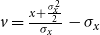 $v=\frac{x+\frac{\sigma _{x}^{2}}{2}}{\sigma _{x}}-\sigma _{x}$
so
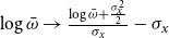 $\log \bar{\omega }\rightarrow \frac{\log \bar{\omega }+\frac{\sigma _{x}^{2}}{2}}{\sigma _{x}}-\sigma _{x}$
and
 $-\infty \rightarrow -\infty$
 \begin{eqnarray*} \int _{0}^{\bar{\omega }}\omega dF\left ( \omega \right ) &=&\frac{1}{\sigma _{x}\sqrt{2\pi }}\int _{-\infty }^{\frac{\log \bar{\omega }+\frac{\sigma _{x}^{2}}{2}}{\sigma _{x}}-\sigma _{xt}}e^{-\frac{1}{2}v^{2}}\sigma _{x}dv \\[5pt] &=&\frac{1}{\sqrt{2\pi }}\int _{-\infty }^{\frac{\log \bar{\omega }+\frac{\sigma _{x}^{2}}{2}}{\sigma _{xt}}-\sigma _{x}}e^{-\frac{v^{2}}{2}}dv \\[5pt] G\left ( \bar{\omega }\right ) &=&\int _{0}^{\bar{\omega }}\omega dF\left ( \omega \right ) ={prob}\left [ \log \omega \leq \frac{\log \bar{\omega }+\frac{\sigma _{x}^{2}}{2}}{\sigma _{x}}-\sigma _{x}\right ] \end{eqnarray*}
For the Dynare code, the following expression can thus be utilized:
 \begin{equation*} G\left ( \bar {\omega }\right ) =normcdf\left [ \frac {\log \bar {\omega }+\frac {\sigma _{x}^{2}}{2}}{\sigma _{x}}-\sigma _{x}\right ] \end{equation*}
Lastly, I need to find the expression for
 $f ( \bar{\omega }_{i} )$
. The probability density function and cumulative distribution function are denoted by
 $f ( \omega )$
and
 $F ( \omega )$
for lognormally distributed
 $\omega$
.
 \begin{equation*} f\left ( \omega \right ) =\frac {dF\left ( \omega \right ) }{d\omega } \end{equation*}
Substitute
 \begin{equation*} \omega =e^{x}=\gt x=\ln \omega \sim N\left ( \mu _{\ln x},\sigma _{\ln x}^{2}\right ) \end{equation*}
 \begin{equation*} =\gt \frac {d\omega }{dx}=e^{x}\rightarrow d\omega =e^{x}dx \end{equation*}
Since
 $\omega$
is lognormally distributed, i.e.
 $x=\log ( \omega )$
is normally distributed, i.e.
 $e^{x}$
is lognormally distributed.
 $\Phi ( \cdot )$
and
 $\phi ( \cdot )$
are the cumulative distribution function and probability density function of the
 $N ( 0,\sigma _{x} )$
distribution, respectively.
 \begin{equation*} f\left ( \omega \right ) =\frac {dF\left ( \omega \right ) }{d\omega }=\frac {d\Phi \left ( x\right ) }{dx}\frac {1}{e^{x}}=\frac {d}{dx}\left [ \Phi \left ( \frac {x-Ex}{\sigma _{x}}\right ) \right ] \frac {1}{e^{x}} \end{equation*}
and
 \begin{eqnarray*} Ee^{x} &=&E\omega =1 \\[5pt] 1 &=&Ee^{x}=e^{\left [ Ex+\frac{\sigma _{x}^{2}}{2}\right ] } \\[5pt] &=&\gt Ex=-\frac{\sigma _{x}^{2}}{2} \end{eqnarray*}
so
 \begin{equation*} f\left ( \omega \right ) =\frac {d}{dx}\left [ \Phi \left ( \frac {x+\frac {\sigma _{x}^{2}}{2}}{\sigma _{x}}\right ) \right ] \frac {1}{e^{x}}=\phi \left ( \frac {x+\frac {\sigma _{x}^{2}}{2}}{\sigma _{x}}\right ) \frac {1}{\sigma _{x}e^{x}} \end{equation*}
Now substitute back
 \begin{equation*} f\left ( \omega \right ) =\phi \left ( \frac {x+\frac {\sigma _{x}^{2}}{2}}{\sigma _{x}}\right ) \frac {1}{\sigma _{x}e^{x}}=\phi \left ( \frac {\ln \omega +\frac {\sigma _{x}^{2}}{2}}{\sigma _{x}}\right ) \frac {1}{\sigma _{x}\omega } \end{equation*}
and
 \begin{equation*} f\left ( \bar {\omega }\right ) =\phi \left ( \frac {\ln \bar {\omega }+\frac {\sigma _{x}^{2}}{2}}{\sigma _{x}}\right ) \frac {1}{\bar {\omega }\sigma _{x}} \end{equation*}
For the Dynare code, the following expression can thus be utilized
 \begin{equation*} f\left ( \bar {\omega }\right ) =normpdf\left ( \frac {\ln \bar {\omega }+\frac {\sigma _{x}^{2}}{2}}{\sigma _{x}}\right ) \frac {1}{\bar {\omega }\sigma _{x}} \end{equation*}
Therefore, the equations characterizing the financial contract will be coded in the following way
 \begin{eqnarray*} 0 &=&\left [ 1-\left ( \bar{\omega }_{it+1}\left [ 1-F\left ( \bar{\omega }_{it+1}\right ) \right ] +G\left ( \bar{\omega }_{it+1}\right ) \right ) \right ] \frac{R_{it+1}^{k}}{ R_{t+1}} \nonumber \\ &+&\frac{1-F\left ( \bar{\omega }_{it+1}\right ) }{1-F\left ( \bar{\omega }_{it+1}\right ) -\mu _{i}\bar{\omega }_{it+1}normpdf\left ( \frac{\ln \bar{\omega }+\frac{\sigma _{xit+1}^{2}}{2}}{\sigma _{xit+1}}\right ) \frac{1}{\bar{\omega }_{it+1}\sigma _{xit+1}}}\left ( \left [ \bar{\omega }_{it+1}\left [ 1-F\left ( \bar{\omega }_{it+1}\right ) \right ] +\left ( 1-\mu _{i}\right ) G\left ( \bar{\omega }_{it+1}\right ) \right ] \frac{R_{it+1}^{k}}{ R_{t+1}}-1\right ) \\[5pt] 0 &=& R_{t+1}\left ( l_{it+1}-1\right ) -\left [ \bar{\omega }_{it+1}\left [ 1-F\left ( \bar{\omega }_{it+1}\right ) \right ] +G\left ( \bar{\omega }_{it+1}\right ) -\mu _{i}G\left ( \bar{\omega }_{it+1}\right ) \right ] R_{it+1}^{k}l_{it+1} \end{eqnarray*}
where I will make use of the auxiliary variables
 $F ( \bar{\omega }_{it+1} )$
,
 $G ( \bar{\omega }_{it+1} )$
, and
 $\sigma _{xit+1}$
, the former representing the sectoral default rate.
 \begin{eqnarray*} F\left ( \bar{\omega }_{it+1}\right ) &=&normcdf\left [ \frac{\log \bar{\omega }_{it+1}+\frac{\sigma _{xit+1}^{2}}{2}}{\sigma _{xit+1}}\right ] \\[5pt] G\left ( \bar{\omega }_{it+1}\right ) &=&normcdf\left [ \frac{\log \bar{\omega }_{it}+\frac{\sigma _{it+1}^{2}}{2}}{\sigma _{xit+1}}-\sigma _{xit+1}\right ] \\[5pt] \sigma _{xit+1} &=&\text{log}(1+(\sigma _{\omega it+1}z_{\sigma t})^{\wedge}{2}) \end{eqnarray*}
The variable
 $\sigma _{xit+1}$
is the sectoral standard deviation of the normal distribution associated to the log-normal distribution
 $\omega _{i}$
with standard deviation
 $\sigma _{\omega it+1}$
which is subject to the risk shock
 $z_{\sigma t}$
.