


1. INTRODUCTION
The race to high intensity beam in linear accelerators has been provoked by the needs in many fields of physics like inertial confinement fusion, tritium production, nuclear transmutation or spallation, neutrino physics, material irradiation in particular for magnetic confinement fusion. Depending on the specifications, the beam is either in continuous wave or pulsed mode, leading to, respectively, large average or peak power, which is given by:
 $$P = \displaystyle{{IE} \over {{n_q}}} $$
where P is the beam power in MW, I is the beam current in A, E is the beam kinetic energy in MeV and n q is the number of charges per particle.
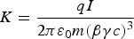
The larger the beam power is, the more harmful beam losses are, and when beam power is very large, even if a tiny part of the beam is lost, it should not be neglected. But high power is not the only consequence of high intensity. High space charge is the other important induced issue that cannot be forgotten. The latter implies strong nonlinear repulsive forces between charged particles of the same sign. The space charge is characterized by the generalized perveance K (Wangler, Reference Wangler2008):
 $$K = \displaystyle{{qI} \over {2{\rm \pi} {{\rm \varepsilon} _0}m{{\lpar {\rm \beta} {\rm \gamma} c\rpar }^3}}} $$
where q and m are the particle's charge and mass, I is the beam peak intensity, ε0 is the vacuum permittivity, β and γ are the relativistic factors, and c is the speed of light in vacuum. Space charge forces, by their strengths, will require a more compact accelerator lattice to prevent quick beam blowup and by its nonlinearity will make beam transportation more delicate, in simulation as well as in operation. The combination of high power and high space charge makes the situation particularly critical: the beam should be controlled very precisely even for its most tenuous part to prevent losses while it is at the same time subject to nonlinear blowup forces difficult to simulate or to control. In this situation, new methods and concepts must be developed to treat the issues induced by high intensity. We can list the main ones as in the following: (1) For high intensity accelerators, not only beam power but also space charge is a concern. Both aspects should be taken into consideration for any analysis of accelerators aiming at comparing their performances and pointing out the challenging sections. (2) High intensity implies substantial beam power at the earliest low energy acceleration sections. Beam losses are critical because even a tiny part of the beam can damage or activate materials. Exhaustive loss predictions are necessary for all the different situations of the accelerator lifetime. (3) High intensity implies strong space charge forces causing beam blowup that must be mitigated by moving the focusing and accelerating components closer. The resulting compactness makes the implementation of beam diagnostic very problematic. A clear strategy for beam measurement has thus to be defined. (4) High intensity implies nonlinear space charge forces at the origin of beam halo generation. The halo has its own dynamics, different from that of the core and plays a significant role in the particle loss process. On the one side, beam optimization must take it into account and aim to match directly the halo part. On the other side, beam characterization must describe not only the core part but also the halo one.
This paper presents advanced concepts and methods for beam analysis, beam loss prediction, beam optimization, beam measurement and beam characterization especially dedicated to very high intensity accelerators. Examples of application of these concepts are given in the case of the IFMIF accelerators.
2. BEAM ANALYSIS
Talking about “high intensity beam” implies first of all to analyze in which extent a given accelerator intensity can be qualified as “high.” There is no absolute threshold value above which the intensity becomes high. Intensity can only be higher or not when comparing to another one and this comparison only makes sense when a higher intensity means explicitly higher challenges we must face. The problem is that in this comparison exercise, high intensity accelerators have often been assimilated to high power ones. Yet, according to Eq. (1), high power can be due to high energy and not necessarily due to high intensity. On the contrary, for a given energy, higher intensity implies higher power. Confusing high intensity and high power may hide all the main difficulties specifically coming from high intensity that should be faced.
Even when studying only the issues purely due to high power, a high power but not high intensity accelerator will reach high power only at high energy and induced issues will mainly concern its last sections, while a high intensity beam may reach substantial power in the very first sections and when is the case, must face important challenges all along the accelerator. Besides, as discussed before, high intensity implies in addition high space charge. To be meaningful, a beam analysis should bring to the foreground these two properties.
Let us take the example of three different proton linacs, called Accel A, B, C characterized by their average, peak intensities and their starting, final energies as following:
Accel A: 125 mA, 125 mA; 0.1 MeV, 40 MeV.
Accel B: 8 mA, 10 mA; 0.05 MeV, 1500 MeV.
Accel C: 40 mA, 0.8 mA; 0.03 MeV, 600 MeV.
It is very common until now to symbolize them as a point in a graph like Figure 1 representing the beam average intensity versus the beam final energy. The beam final power calculated with Eq. (1) is shown as the dashed lines of same power 0.1, 1, 10 MW. This graph may suggest that Accel B will face the worst issues, followed by Accel A then Accel C. But this is not totally true, because of at least two reasons: (1) Only the last sections are concerned. The upstream sections may face important difficulties or not, independently from the final one. This graph does not allow knowing about them. (2) The other issue, the beam space charge is not considered. It cannot be deduced from this graph as it depends on the peak intensity and not on the average one.
Beam average intensity versus beam final energy.

This kind of graph is highly reductive. It may lead to wrong estimates of the difficulties in the first sections and may hide the difficulties due to high space charge.
We propose instead to use the set of two graphs in Figure 2 representing the beam power and the generalized perveance versus the beam energy along the accelerator. It appears that for a given energy, i.e., for a given section of the accelerator, the Accel B beam power is indeed higher than that of Accel C, but from the space charge point of view, Accel C will face much more beam nonlinearities, thus halo, beam loss problems than Accel B. For its part, Accel A will have to face the worst issues. For a given energy, not only its beam power is higher but its space charge effects too. The combination of the two graphs allows highlighting even more the critical aspect of the encountered difficulties. When considering a given beam power, for example 1 MW, the Accel A general perveance is more than 100 (respectively 1000) times higher than that of Accel C (respectively Accel B). That means that when the beam power is so high that even a tiny loss, i.e., 10−6 of the beam, is critical, a very precise control of the beam is needed and the beam behavior remains very difficult to predict.
Beam power and generalized perveance as functions of beam energy along the accelerators.
Further detailed analysis can be carried out when considering each section of the accelerators. Indeed, accelerators often use typical sections for accelerating and focusing particles: particle Source, LEBT, RFQ, MEBT, Linacs, and HEBT. Depending on beam power and space charge, decisions can be taken to pass from a section to another at a chosen energy. The graph in Figure 1 allows knowing only about the beam power at the last Linac end and the HEBT. The two graphs of Figure 2 can be used to make meaningful comparisons between different accelerators for all the sections. This allows, right at a design stage, either to be aware that the considered section is really challenging because the beam power or/and space charge is/are higher than those of all other accelerators, or else to adjust the section starting/final beam energy in order to deal with beam power or space charge in the same range as existing accelerators. For example, the Accel C starting energy 0.03 MeV is very low, implying a huge space charge effect, even higher than that of Accel A. A quick look at the second graph of Figure 2 lets us know immediately that for their respective intensities, if the Accel C extraction source can go up to 0.05 MeV, its space charge will be the same as of Accel A at extraction. Similarly, if the Accel B RFQ final energy is 3 MeV, the one of Accel A RFQ must be only 0.25 MeV (which is very easy) in order to have the same beam power, or up to 14 MeV (which is very difficult) in order to have the same space charge. For higher energies, considerations of beam energy and power will help to decide on the nature of accelerating cavities to use: HWR, Spoke, Elliptical, etc.
Applications of the two graphs discussed here to some high intensity accelerators, achieved, under construction or planned, are shown in Figure 3 (Nghiem et al., Reference Nghiem, Chauvin, Comunian, Delferrière, Duperrier, Mosnier, Oliver and Uriot2011a). Similar graphs but representing peak power or energy instead, may be useful for accelerators with very high instantaneous beam power like intense heavy ion accelerators for inertial fusion purposes or for beam-plasma physics (Bangerter et al., Reference Bangerter, Faltens and Seidl2013; Hoffmann et al., Reference Hoffmann, Blazevic, Ni, Rosmej, Roth, Tahir, Tauschwitz, Udrea, Varentsov, Weyrich and Maron2005).
Beam power and generalized perveance as functions of beam energy along typical high intensity accelerators worldwide, achieved or under construction or planned.
3. BEAM LOSS PREDICTION
High intensity beam can imply high beam power at the earliest energy stages and the high power part can concern almost the whole accelerator. In such a case, beam losses, even when they represent a small fraction of the beam, can take away a significant power. Those losses, when they are accidental, can damage equipment surrounding the beam via heat deposition, or when they last a long time, can activate materials and induce harmful radiation for personnel. If superconducting equipment is concerned, cryogenic systems must be able to evacuate the deposited heat. That is why, for designing personnel or machine protection systems, cooling systems or for fixing the limitations to be kept during certain beam manipulations, it is necessary to predict possible beam losses during all the possible situations the accelerator will encounter, accidental or not. The double issue is to define as exhaustively as possible all the typical loss situations in the accelerator lifetime and to define the procedure to simulate and estimate them. After many studies, it appears to us that the situations and the protocols described in the following should be enough: (1) Ideal machine; (2) Starting from scratch; (3) Beam commissioning, tuning, exploration; (4) Routine operation; (5) Sudden failure.
(1) Ideal machine. “Ideal” means here nominal theoretical conditions, without any error. That should correspond to a machine where all the technical components are perfectly fabricated and aligned, or else perfectly corrected at the source, and the beam has been perfectly tuned. Losses in such conditions should be minimum, we cannot hope to have less. These are minimum and permanent losses that have to be withstood. They are obtained by a start-to-end simulation at nominal tuning without any error.
(2) Starting from scratch. In this condition, no correction has yet been applied, while we can expect that: (a) The technical components have been fabricated and aligned as specified, within the already defined tolerance ranges. (b) The tunable parameters (fields and gradients) are set at their nominal theoretical values. We must however expect that the real beam behavior is not exactly the same as theoretically simulated, due to nonlinear space charge forces. This theory-reality difference can be roughly estimated as equivalent to field and gradient variations in a given range (for example, ±10%) of their nominal values, according to the beam dynamics optimization results obtained in different working configurations since the beginning of the project.
Losses when starting from scratch can thus be estimated by performing a number of (for example, 500) start-to-end simulations without any correction in the presence of random “errors” of two kinds: mechanical, alignment errors randomly distributed within tolerances and tunable parameter errors (gradients, fields) randomly distributed within a range (for example, ±10%) of their nominal values.
Losses for each location along the accelerator are then collected for all the simulated cases, from which curves of loss probability can finally be deduced.
(3). Beam commissioning, tuning, exploration. This occurs during beam commissioning or whenever the beam operation is not as satisfying as theoretically expected in such a way that a beam tuning is necessary, or else when an exploration around a nominal setting is desirable. Those situations take place at different epochs of the accelerator life. However, the induced beam losses can be calculated in the same way. As in the previous case 2, we can assume mechanical errors within tolerances and tunable parameter variations of about ±10%. The only difference is that now the trajectory is corrected. Losses can thus be quantified by the same simulations as in the case 2, but with trajectory correction.
(4) Routine operation. This can be performed when the beam characteristics are satisfying, i.e., as theoretically expected with all the parameters, mechanical and tunable parameters, as specified within tolerances and the trajectory corrected. Losses can thus be calculated by performing a number of (for example, 500) start-to-end simulations with all the errors within tolerances, in the presence of trajectory correction.
(5) Sudden failure. These accidental situations are not easy to be exhaustively studied, especially when a combination of different failures can lead to more important losses than an individual failure. Reflections and analysis should be carried out for each subsystem to detect what is the worst case, what is the main affected location or equipment, when one tunable parameter (gradient, field, phase, RF power, pressure…), or a given combination of them, are suddenly switched off. But attention should also be paid to detect if there is an intermediate case which can induce more losses, for example, in the transition from the nominal value to zero for specific field or gradient. At least, two extreme cases can be studied: failure of individual components and global failure of all the components at once, from 110% to 0% of their nominal values. This can be due to power supply failures that accidentally provide a larger power or that can be suddenly switched off, making the fields or gradients returning progressively to zero.
A complete “catalogue of losses” has been obtained following the above protocol for the IFMIF Prototype accelerator (Nghiem et al., Reference Nghiem, Chauvin, Comunian, Oliver and Uriot2014c). Examples of results at full power are given in Figures 4 and 5, which, respectively, show beam loss probability in case of starting from scratch and beam loss in case of sudden failure of the second solenoid of the LEBT. Such results are meant to be starting points for assessing all the accelerator safety aspects. It should concern all the accelerator subsystems about the identified hot points to be protected or cooled down (facing beam equipment and diagnostics), the machine protection system about the requested velocity for the beam stop procedure, the control system about the limitations to impose to power supply variations and the beam operation about the maximum beam power, i.e., intensity or duty cycle, to be planned depending on each situation. If only a very small beam power is acceptable, a specific beam chopper can be needed and beam diagnostic performances should be checked for such a faint beam.
Beam loss power probabilities when starting from scratch for a full-power beam (statistics over 500 machines) of the IFMIF Prototype accelerator. The bottom figure is a zoom of the top one.
Beam loss power in case of sudden failure of the second LEBT solenoid of the IFMIF Prototype accelerator. The solenoid field can go suddenly up to 110% or down to 0% of its nominal field (100%), by steps of 5%.
Notice that beam losses are also a concern in case they are a limitation factor for achieving the very high intensity necessary for ion fusion scenarios. An example of detailed beam loss studies in such a context can be found in Mustafin et al. (Reference Mustafin, Boine-Frankenheim, Hofmann and Spiller2002), where are considered secondary neutron production due to lost ions and vacuum pressure instability due to charge exchange losses.
4. BEAM OPTIMIZATION
The very first question for beam dynamics optimization when studying or designing a linear accelerator is: what are the parameters to be optimized?
As beam optimization is in any case time consuming, it is currently enough to target the statistic parameters of the particle population, namely the emittance and the Twiss parameters, which respectively characterize the global extension and angles of inclination of the beam in the phase space. For a given position along the accelerator, instead of dealing with each particle coordinate, only a few parameters must be taken care of. As nonlinear space charge forces will induce emittance growth and halo formation, the idea was to minimize this emittance growth as much as possible. For that, many studies have been undertaken, leading to recommendations to avoid energy transfer between transverse/longitudinal movements and to match the input beam to a focusing structure, all of them regarding emittance, Twiss parameters or phase advance.
Yet, the final goal is to minimize halo, not emittance, in order to prevent beam losses, and the relation between emittance and halo is not straightforward. In Allen and Wangler (Reference Allen and Wangler2002), it is pointed out that there could be emittance growth without halo growth but halo growth always implies emittance growth. So the above recommendations are likely to be efficient only in case of moderate space charge. For very intense beams, they are difficult to apply. The reason is that the classical statistical parameter set is not enough to represent the beam. In Nghiem et al. (Reference Nghiem, Chauvin, Counienc and Oliver2011b), it is proven that two different beam distributions of 125 mA–9 MeV D+ particles characterized by the same emittance and twiss parameters become significantly different after being transported through only three quadrupoles. Figure 6 shows the results obtained with the TraceWin code (Duperrier et al., Reference Duperrier, Pichoff and Uriot2002) simulating 106 macro-particles at the IFMIF HEBT entrance. Beam transport is clearly distribution dependent. Therefore, matching a beam to a structure when considering only its global parameters is not sufficient.
Two different beam distributions of 125 mA–9 MeV D+ particles characterized by the same emittance and Twiss parameters transported 3.5 m downstream through only three quadrupoles. Top: Gaussian beam. Bottom: IFMIF nominal beam at the SRF-Linac exit. At the output, the two beams are significantly different, by their visual aspect and their emittance and Twiss parameters.
Some attempts aim to directly mitigate the halo, as for example using a round input beam (Jeon, Reference Jeon2013) or using the transverse-longitudinal coupling resonance to get rid of the longitudinal halo (Hofmann, Reference Hofmann2013). We propose to use a radical method called “halo matching” aiming to smooth the extension of the external border of the beam, thus directly minimizing the halo (Chauvin et al., Reference Chauvin, Duperrier, Mosnier, Nghiem and Uriot2009). The method consists in minimizing the radial extension of the most external macro-particles, at locations where it is the largest, i.e., at focusing elements, tuning all of the lattice in this purpose. We call it “halo matching.” This multi-parameter optimization is time consuming. Furthermore, contrarily to classical methods where it is enough to match the input beam to a given focusing channel, the present optimization also tunes the whole channel itself, and this must be re-done whenever the particle distribution at entrance changes. A specific code has been written for that, using the particle swarm optimization procedure (Kennedy & Eberhart, Reference Kennedy and Eberhart1995), suitable for searching the lowest minimum of an n-Dimension surface having several local minimums. An example of successful result is given in the top of Figure 7 for the superconducting radio frequency (SRF) linac of the IFMIF accelerators, where a CW-125 mA D+ particles are accelerated from 5 MeV to 40 MeV, corresponding to beam powers from 0.6 to 5 MW. The consequence of this halo matching procedure is a significant emittance growth as shown in the bottom of Figure 7. As an exercise, an alternative tuning has been obtained by applying in the second part of the structure the classical method of minimizing emittance growth consisting in avoiding the transverse-longitudinal coupling resonance (Nghiem et al., Reference Nghiem, Chauvin, Comunian, Delferrière, Duperrier, Mosnier, Oliver, Simeoni and Uriot2014a). We can call it “emittance matching.” The emittance growth is indeed reduced, but at the expense of an important halo growth (Fig. 8). This shows the limit of classical methods that consider beam emittance as the critical parameter. Considering the halo as the figure of merit is likely more appropriate for high intensity accelerators.
Radial density and RMS normalized emittance of the IFMIF beam along the four cryomodules of the SRF Linac. Results obtained by the halo matching procedure using 106 macro-particles, consisting in minimizing the extension of the outermost particles.
Same as Figure 7 but obtained by the emittance matching procedure, consisting in avoiding the transverse-longitudinal resonance in order to minimize emittance growth.
The above beam was simulated and optimized with 106 macro-particles which is the minimum number of particles to be considered as we must ensure that below 1 W/m is lost as required (it has been checked later on that this result holds for the actual number of particles, 4.5 109 in each bunch). This means that well below 1 particle over 106 can be lost. We call these losses “micro-losses.” The problem is that beam dynamics transport codes are not reliable or precise to the level of 10−6. Furthermore, the present very strong space charge effects have never been benchmarked, making the simulation results especially questionable. That is why these results can simply be seen as a theoretical proof that such a required performance is feasible. In order to make them really achievable, a corresponding online fine tuning procedure should be found, with dedicated diagnostics. But on their side, diagnostic devices in a high intensity accelerator encounter themselves serious issues. This will be discussed in the next section.
5. BEAM DIAGNOSTICS
As pointed out in Section 1, the challenge induced by high intensity is two-fold, high power and strong space charge. The resulting issues for beam measurement are developed in the following (Fig. 9). (1) With high power, even tiny losses must be avoided. Typically, as only well less than 1 W/m losses are tolerated to meet hands-on maintenance requirements (Mokhov & Chou, Reference Mokhov and Chou1999; Sugimoto & Takeuchi, Reference Sugimoto and Takeuchi2004), a MW beam should be controlled at a much better level than 10−6. But at this level of precision, beam dynamics simulations are definitely not reliable and accelerator equipment are absolutely not reproducible. On top of that, strong space charge implies strong nonlinear effects making beam optimization furthermore delicate and beam tuning highly sensitive. Therefore, in order to achieve the required performances for the beam, online machine tuning based on beam diagnostics is mandatory and should be expected to occur rather frequently. (2) Beam high power also implies higher deposited power on diagnostic devices. Typically, a MW beam can induce hundreds kW deposited on interceptive diagnostics, in such an extent that the latter cannot be used. Only sophisticated and bulky non-interceptive diagnostics are possible at full power. But strong repulsive space charge forces compel to substantially compact the accelerator structure in order to mitigate beam blow up, emittance growth and halo formation. Consequently, there is a severe lack of space for installing diagnostic devices. The overall result is that installation of diagnostic devices is difficult or even not possible. (3) To summarize, we are clearly in the presence of conflicting issues: on the one hand, diagnostics are not only necessary for beam characterization but also critical for achieving targeted performances; on the other hand, their implementation is difficult or not possible.
Diagnostic issues in the context of high intensity.
Contrarily to current accelerators where diagnostics can be installed almost without restriction, high intensity accelerators force to define a clear strategy for beam measurements to be possible. We propose to adopt a twofold strategy: (1) Can only be used for the beam dynamics optimization methods that have an online avatar, a similar tuning procedure on the real machine associated with appropriate diagnostics in sufficient quantity. For example, the injection into the RFQ is recognized as optimum for an input beam characterized by well-defined emittance and Twiss parameters. The latter holds even in the presence of strong space charge because of the very strong focusing in the RFQ, resulting in a very small beam, destined to literally kill space charge effects. But there is absolutely no room for installing diagnostics capable of measuring these phase space parameters. This is why we propose to optimize directly the RFQ transmission which can be reproduced online with the help of current transformers installed immediately before and after the RFQ. And we have verified with multi-particle simulations that this method leads to the same requirement of input emittance and Twiss parameters (Chauvin et al., Reference Chauvin, Delferrière, Duperrier, Gobin, Nghiem and Uriot2012). Another example is the halo matching procedure presented in Section 4. The objective being avoiding micro-losses at focusing elements, we asked for diagnostics installed all around those locations, small and close enough to the beam, so that they can be used to acquire sufficient independent micro-loss data to be minimized by varying the focusing forces. After dedicated studies, chemical vapor deposition diamonds (Marroncle et al., Reference Marroncle, Abbon, Egberts and Pomorski2011) are found to be the most appropriate diagnostic for micro-loss measurement meeting the requirements. (2) Clearly distinguish between “essential” diagnostics and “characterization” diagnostics. “Essential” diagnostics are necessary for commissioning, tuning, and operating the accelerator in order to meet the required specifications of beam current and losses. They should be available on a day-to-day basis for beam tuning at full power, thus non-interceptive. Their performances will directly impact the achievement of the accelerator specifications. “Characterization” diagnostics are useful for beam study during commissioning, or for the understanding of beam behavior relative to beam dynamics simulations. If the available room is short, they could be available only during the sequential commissioning stages. If full power cannot be handled, they could be used only for low duty cycle.
For the IFMIF accelerators, for example, the measurements considered as “essential” are beam position, phase, current, losses and micro-losses, while “characterization” measurements are transverse profile, emittance, halo, energy spread, mean energy, bunch length. In this case, microloss is essential and not emittance, but it could be differently for another accelerator. Depending on the accelerator purposes or performance requirements, these two lists should be re-arranged.
6. BEAM CHARACTERIZATION
Particle beams have ever been characterized either by the six-dimensional coordinates of each particle or macro-particle, which is a huge number of data, or else by its statistical moments, namely the emittance and Twiss parameters, of which a combination gives the RMS size also called beam envelope.
Increasingly high intensity progressively shows the limit of the latter global parameters which consider the beam as a whole. As discussed above, high power compels to focus on losses or micro-losses coming from the beam external part, the halo. This halo is created or boosted by the nonlinear space charge forces. Because its density is much lower than the core's and submitted to a different space charge field regime, rather nonlinear compared to the rather linear one in the core, the halo is transported differently from the core along the focusing structure. There is a growing need to characterize separately the core and the halo parts of the beam. The global emittance or RMS size does not meet this need as either they rather characterize the core when the halo size is small or else the halo when its size is well bigger than that of the core.
Intensive works have been launched for decades from the initial studies of Chen and Davidson (Reference Chen and Davidson1994), Gluckstern (Reference Gluckstern1994), Chen and Jameson (Reference Chen and Jameson1994) aiming at studying the halo. Theoretical studies have identified the causes of halo formation and growth, some of them having been confronted to halo measurements (see references in Nghiem et al., Reference Nghiem, Valette, Chauvin, Pichoff and Uriot2014d). As explained in Section 4, a specific optimization procedure has been developed to minimize the halo. However, no clear definition of halo has emerged. Most of the cited studies are based on visual inspection and often assimilate the beam total size and the halo. When noticing halo decreasing or increasing, it is not clear that this is also due to the variation of the beam core or not, for the simple reason that there was no clear distinction between core and halo. An international workshop especially dedicated to the halo (Wei et al., Reference Wei, Fischer and Manning2003) concluded that a general definition of beam halo could not be given and only mentioned some halo parameters consisting in comparing the far-from and close-to center parts of the beam, as for example comparing the 90% or 99%, etc. emittance to RMS. Another parameter often used to characterize the halo is the “h parameter” (Wangler & Crandall, Reference Wangler and Crandall2000; Allen & Wangler, Reference Allen and Wangler2002) which is based on the kurtosis of the density profile, presupposing that, like the kurtosis, the halo is bigger for a peaked profile than for a flat one.
Recently, we proposed a precise determination of the core-halo limit (Nghiem et al., Reference Nghiem, Chauvin, Simeoni and Uriot2014b). The idea is to extrapolate from the case of dense uniform core surrounded by a much more tenuous halo (see Fig. 10). In this extreme case, the space charge field is clearly linear in the core and nonlinear in the halo, and the limit between core and halo is obviously the location where there is the abrupt slope variation in the profile when going from a tenuous density to a much higher one. For a general density profile with continuously varying slope, we propose to determine the core-halo limit as the location of biggest slope variation, that is where the second derivative is maximum (not to be confused with the inflection point that is given by the second derivative zero). This determination can be extended to an n-dimension space by considering for example the Laplacian maximum (studies are undergoing). This determination has a quadruple advantage: (1) It can be applied to any type of density profile, see examples in Figure 11; (2) It corresponds well to a visual inspection of the profile; (3) It does not presuppose any relation between the halo and the general shape of the profile; (4) And, most important of all, the core and the halo so defined are located in the two different space charge field domains or, said with other words, such a limit reveals the internal dynamics of the particle beam (Nghiem et al. Reference Nghiem, Valette, Chauvin, Pichoff and Uriot2014d).
Uniform and continuously varying density profiles with their corresponding second derivatives.
Beam density distribution at some key positions along the IFMIF Prototype accelerator. Top: Density in the transverse plane (x,y) with its projection profiles in x and y directions. Down: Density profile in x and its 1st and 2nd derivatives.
Once this limit determination is extended to a n-Dimension space, especially in the two-dimensional, four-dimensional, or six-dimensional phase spaces, the core and the halo may be characterized by their own emittance and Twiss parameters, which allows to study in parallel their evolution along the accelerator. For the moment, in one-dimensional, such a beam characterization can already be appreciated. In the three graphs on the top of Figure 12 is presented the IFMIF beam along the Prototype accelerator characterized in a classical way that is by its emittance, RMS size and h-parameter. The first two graphs only give a global view of the beam extension. They could be replaced by one graph showing the external limits of the core and of the halo, which exhibit precisely the extensions of the two main components of the beam (Fig. 12-bottom). The third graph gives an abstract parameter presumably related to the halo importance. It could be replaced by two graphs giving precisely the halo importance in size and in number of particles, namely PHS and PHP, respectively the percentages of halo size and halo particles.
Beam characterization in horizontal (x, red) and longitudinal (z, green) along the IFMIF-Prototype accelerator, from source extraction to final beam dump.
Top: Classical characterization by (1) beam envelope, (2) RMS emittance, (3) halo parameter.
Down: Proposed characterization by one-core and halo limits (internal and external lines of same color in the graph), 2% of halo size, 3% of halo particles.
Typically, this kind of characterization allows analyzing clearly and precisely the differences between the two procedures of halo matching and emittance matching discussed in Section 4. See Figures 13 and 14, related respectively to Figures 7 and 8. It is clear that halo matching leads to a smaller beam total size including halo, while emittance matching leads to less coupling, less beat between transverse and longitudinal oscillations. Halo matching has the advantage of reducing the halo and the core sizes at once, but implies more particles in the halo. And vice versa for emittance matching. Anyway, these characterizations appear to be relevant to analyze a high intensity beam where the halo should not be neglected and in particular for the purpose of limiting risks of losses. Ideally, in the general case, the total beam size as well as PHS and PHP should be minimized. When this is hard to achieve, some of these constraints can be relaxed, depending on the objective. For a short structure that can be optimized as a whole, minimizing the beam total size is enough to prevent losses. For a longer structure, PHS and then PHP, in this order of priority, must be minimized in order to avoid a too important development of the halo that could induce losses later on downstream.
Beam characterization of the IFMIF beam along the four cryomodules of the SRF Linac. Results obtained by halo matching as in Figure 7.
Beam characterization of the IFMIF beam along the four cryomodules of the SRF Linac. Results obtained by emittance matching as in Figure 8.
7. CONCLUSIONS
High intensity beams imply high power and strong space charge. Both aspects should be taken into account when analyzing the induced issues along the accelerators. The combination of the two aspects imply new and serious issues, forcing to study advanced methods and concepts: catalogue of losses, halo matching, micro-losses, online avatars of beam dynamics optimizations, essential and characterization diagnostics, core-halo limit, PHS, PHP. Those new approaches have been proposed and compared to the classical ones in use until now, for the five purposes of beam analysis, beam loss prediction, beam optimization, beam diagnostic and beam characterization.



