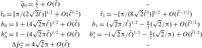
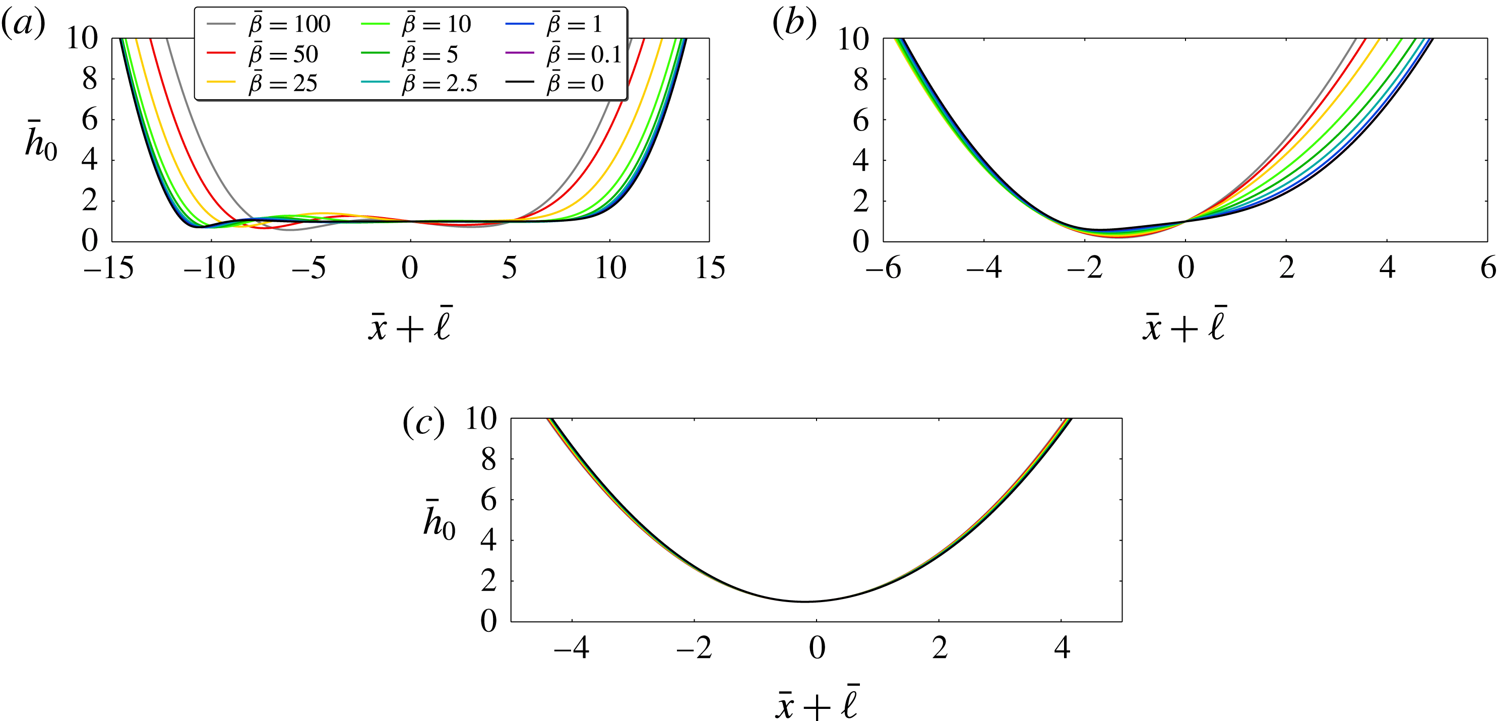
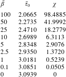
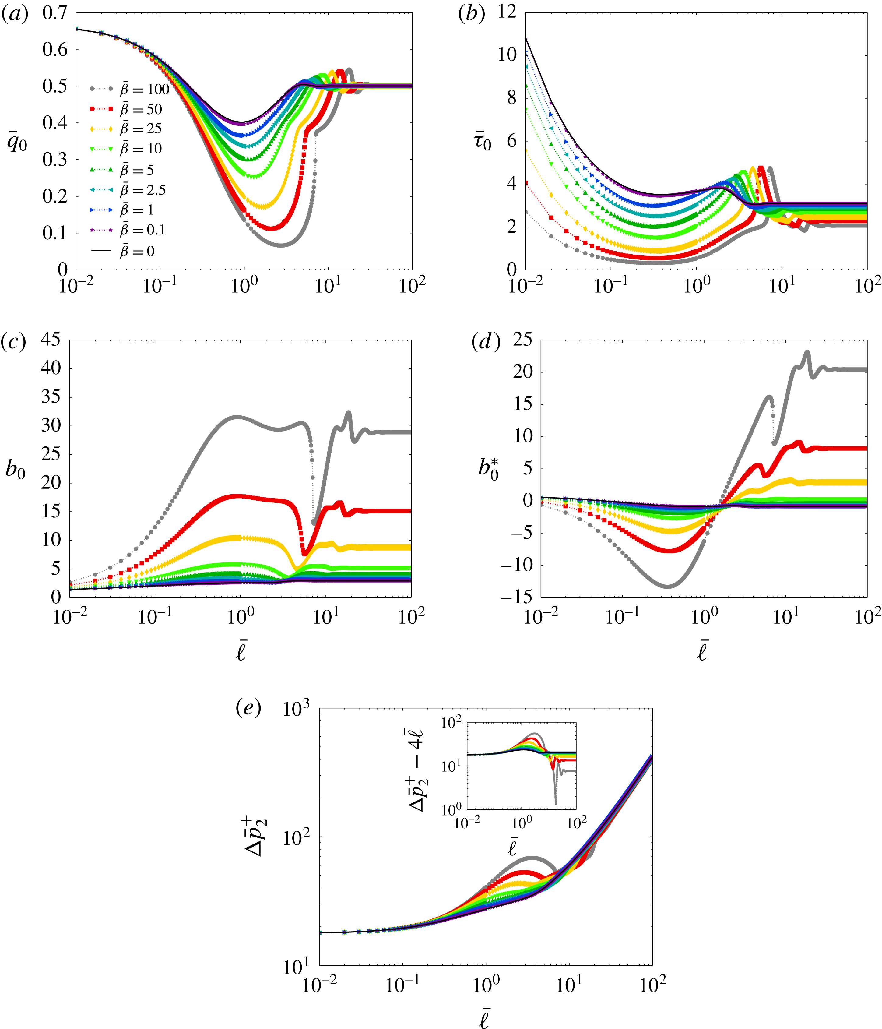
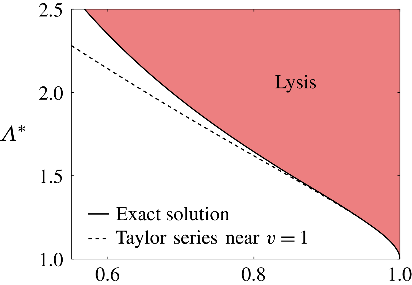
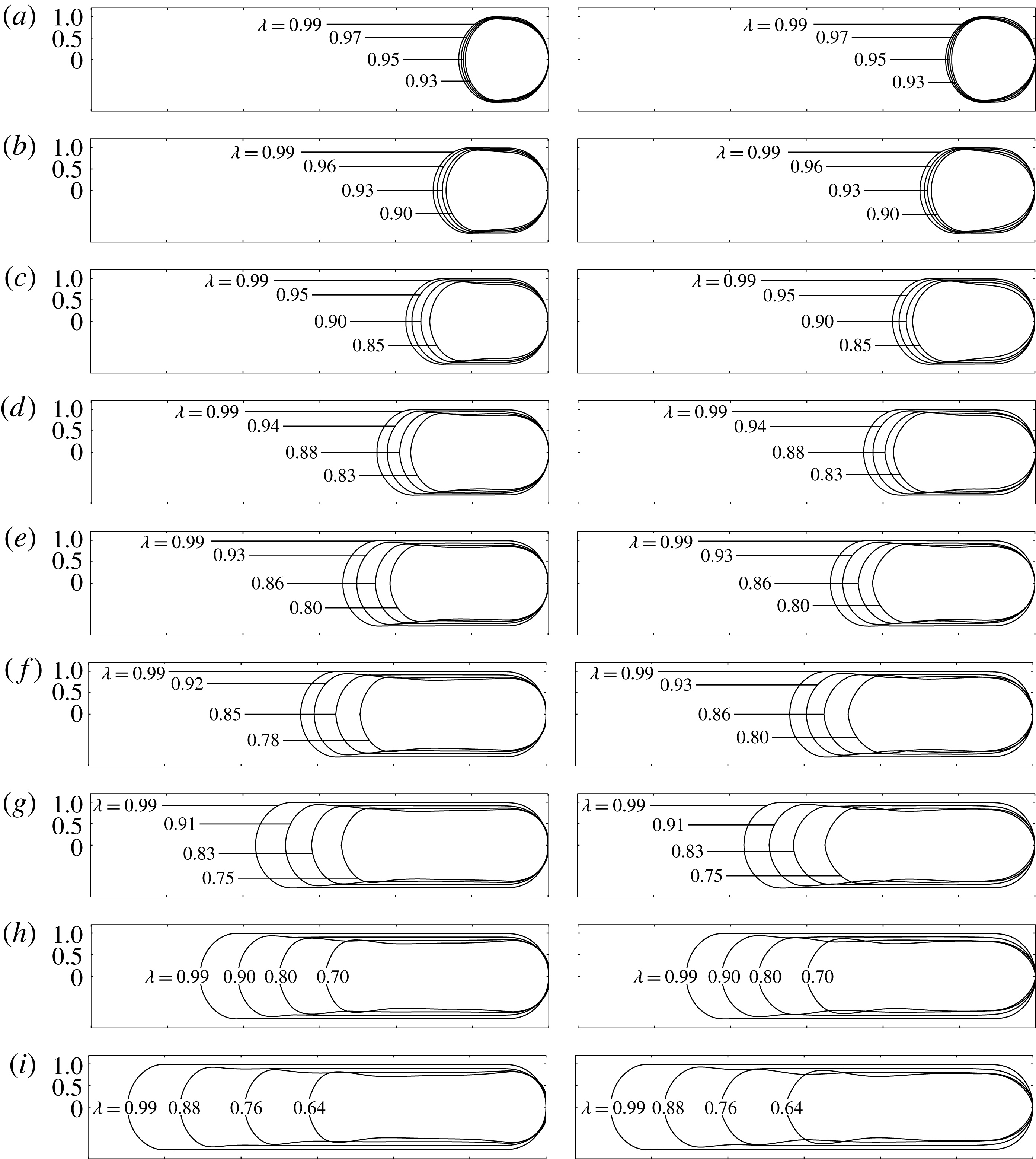
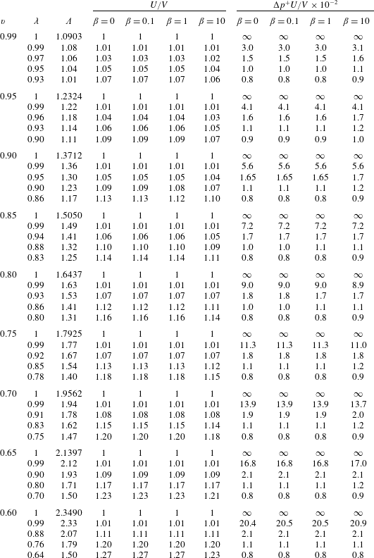
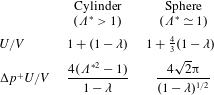
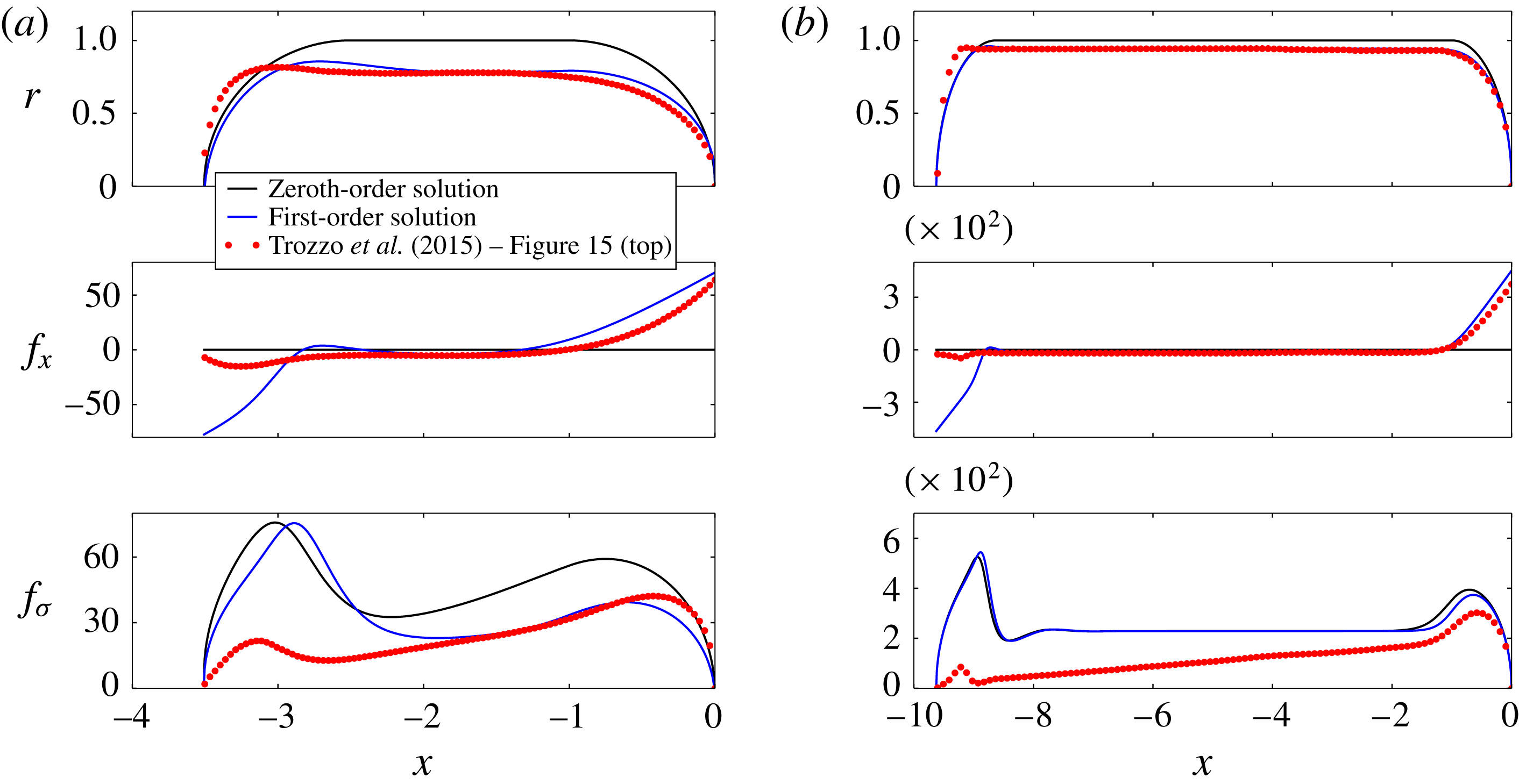
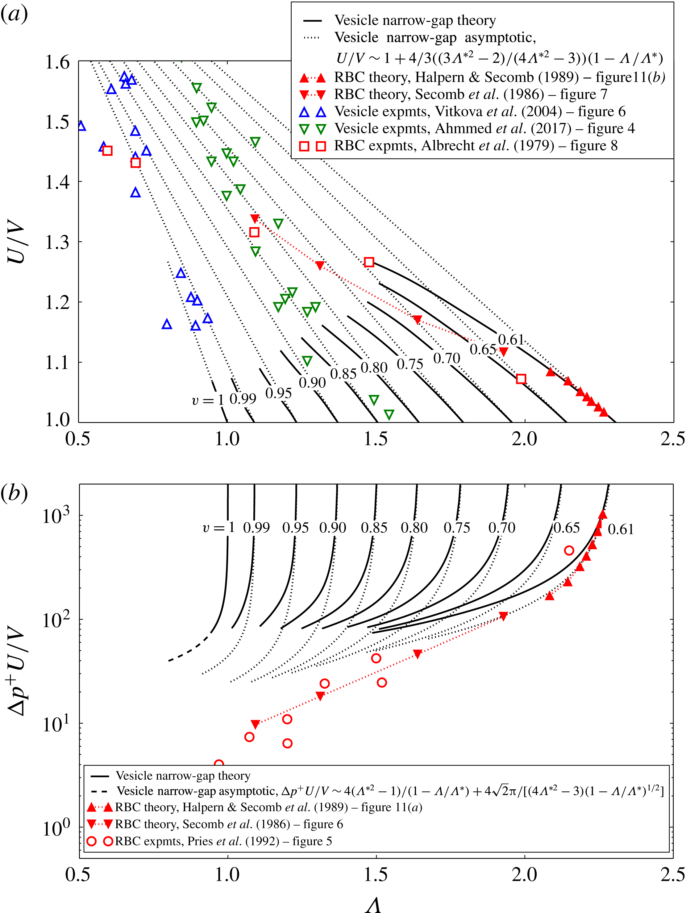
1 Introduction
Squeezing a cell through a narrow, fluid-filled conduit facilitates measurement or alteration of its mechanical properties (Hochmuth Reference Hochmuth2000). Recent work with mammalian cells has shown that mechanically induced poration by controlled squeezing can enhance the permeability of the cell membrane, enabling the uptake of macromolecules for targeted delivery applications (Sharei et al.
Reference Sharei, Zoldan, Adamo, Sim, Cho, Jackson, Mao, Schneider, Han and Lytton-Jean2013). However, severe deformation by squeezing can lead to catastrophic rupture of the membrane (Mohandas & Evans Reference Mohandas and Evans1994). Experimental measurements of the extra pressure drop
 $\unicode[STIX]{x0394}p^{+}$
required to push a single cell at a speed
 $U$
through a conduit indicate that membrane rupture occurs at a critical value of the dimensionless extra pressure drop
 $\unicode[STIX]{x0394}p^{+}R/(\unicode[STIX]{x1D707}V)$
, where
 $\unicode[STIX]{x1D707}$
is the suspending fluid viscosity,
 $V$
is the mean speed of the suspending fluid and
 $R$
is the hydraulic radius of the conduit (Abkarian, Faivre & Stone Reference Abkarian, Faivre and Stone2006; Abkarian et al.
Reference Abkarian, Faivre, Horton, Smistrup, Best-Popescu and Stone2008). Theoretical predictions of the speed ratio
 $U/V$
and dimensionless extra pressure drop
 $\unicode[STIX]{x0394}p^{+}R/(\unicode[STIX]{x1D707}V)$
, as functions of the dynamical and geometrical parameters of a flow system, are therefore imperative to the rational design of experiments meant to probe cell-mechanical properties by cell squeezing.
Early models of a single, freely suspended cell flowing through a narrow conduit with minimal clearance were developed by treating the cell as a rigid particle and invoking lubrication theory to describe the flow in the suspending fluid (Lighthill Reference Lighthill1968; Hochmuth & Sutera Reference Hochmuth and Sutera1970; Bungay & Brenner Reference Bungay and Brenner1973). Bretherton (Reference Bretherton1961) had previously applied lubrication theory to the motion of a large bubble in a circular tube. In the 1970s, researchers began to borrow concepts from thin-shell mechanics in modelling the continuum-elastic properties of biological membranes, with particular attention paid to ‘model cells’ such as red blood cells and vesicles. Secomb et al. (Reference Secomb, Skalak, Oozkaya and Gross1986) and Halpern & Secomb (Reference Halpern and Secomb1989) extended Bretherton’s theory to the motion of a single red blood cell in a circular tube, treating the cell as a sac of fluid enclosed by an incompressible, elastic sheet with a two-dimensional shear modulus
 $G$
and bending modulus
 $B$
. Quéguiner & Barthès-Biesel (Reference Quéguiner and Barthès-Biesel1997) and later Pozrikidis (Reference Pozrikidis2005) performed high-fidelity numerical simulations of red blood cells in tube flow using the boundary element method.
Vesicles are distinct from red blood cells in that they lack a spectrin-actin cortex, so their membranes are internally fluid with vanishing shear elasticity (
 $G=0$
). Helfrich (Reference Helfrich1973) posited that the lipid-bilayer membrane of a vesicle be treated as a two-dimensional, incompressible fluid with a finite bending stiffness
 $B$
. Adopting Helfrich’s constitutive model, Bruinsma (Reference Bruinsma1996) was the first to devise a lubrication theory for the motion of a long, closely fitting vesicle in a capillary tube. Despite some important findings, Bruinsma’s theory suffers from several shortcomings. For one, he concluded that membrane bending elasticity had no impact on the extra pressure drop
 $\unicode[STIX]{x0394}p^{+}$
regardless of the vesicle speed
 $U$
, in contrast with the findings of Secomb et al. (Reference Secomb, Skalak, Oozkaya and Gross1986). Secondly, for large vesicle speeds he concluded that
 $\unicode[STIX]{x0394}p^{+}$
should be of
 $O(\unicode[STIX]{x1D707}UL^{3}/R^{4})$
, where
 $L$
is the vesicle length. This order assignment predicts a cubic dependence on
 $L$
and shows no dependence on the lubricating gap thickness
 $h$
, both of which are anomalous findings. By contrast, Halpern & Secomb (Reference Halpern and Secomb1989) deduced the more reasonable order assignment
 $\unicode[STIX]{x0394}p^{+}=O[\unicode[STIX]{x1D707}UL/(Rh)]$
for a long red blood cell.
Subsequent experimental measurements (Vitkova, Mader & Podgorski Reference Vitkova, Mader and Podgorski2004) and coarse-grained simulations (Noguchi & Gompper Reference Noguchi and Gompper2005) of vesicles in capillary flow have focused on situations where the vesicle is only moderately confined. More recent boundary element simulations from Trozzo et al. (Reference Trozzo, Boedec, Leonetti and Jaeger2015) have yielded predictions for the vesicle shape – though not the hydrodynamical quantities
 $U/V$
and
 $\unicode[STIX]{x0394}p^{+}R/(\unicode[STIX]{x1D707}V)$
– at various degrees of confinement. These studies have proved to be useful, but the dearth of available measurements or theories for vesicles flowing in narrow conduits leaves the aforementioned issues with Bruinsma’s theory unresolved.
The purpose of the present work is to develop a rigorous theory for the motion of a freely suspended, closely fitting vesicle in a circular tube. The main objective is a prediction for the speed ratio
 $U/V$
and dimensionless extra pressure drop
 $\unicode[STIX]{x0394}p^{+}R/(\unicode[STIX]{x1D707}V)$
in situations where the clearance between the vesicle membrane and the tube wall is small. This regime is difficult to access via high-fidelity numerical simulations due to the necessity of extremely refined grids within the narrow gap. Although the Helfrich constitutive law is used to model the vesicle membrane, the present theory differs from Bruinsma’s in several important ways. For one, in lieu of directly applying the equations of lubrication theory, the basic equations of viscous flow are first presented in their most general form and later expanded under the auspices of a formal perturbation theory. This approach enables computation of corrections to the lubrication approximation. Secondly, rather than assume that the vesicle is long, as is usually done in the analysis of large bubbles in capillary tubes (Bretherton Reference Bretherton1961; Ratulowski & Chang Reference Ratulowski and Chang1990; Wilson Reference Wilson1995), the length of the vesicle is included as a parameter and vesicles of intermediate size are considered. Finally, the effect of bending elasticity on the vesicle’s motion is elucidated. Previously reported results for red blood cells (Secomb et al.
Reference Secomb, Skalak, Oozkaya and Gross1986; Halpern & Secomb Reference Halpern and Secomb1989) are clarified and extended, and the apparent discrepancies with Bruinsma’s theory are resolved.
This paper is organized in the following way. In § 2, the basic equations are presented in their most general form. The equations are rendered dimensionless in § 3, yielding four dimensionless parameters that govern the flow system. In § 4, the dimensionless equations are expanded in the so-called ‘narrow-gap limit’, yielding a singular perturbation problem. The perturbative solution is derived in § 5, including higher-order corrections. Two particular asymptotic limits, neglecting the effect of membrane bending elasticity, are considered in § 6: one in which the vesicle is long and cylindrical, the other in which it is short and spherical. The effect of membrane bending elasticity is then examined in § 7. In § 8, the gap thickness and vesicle length are eliminated as parameters, leading to an alternative (and useful) parametrization of the theoretical results. A discussion of the results is presented in § 9. Concluding remarks are given in § 10.
2 Basic equations
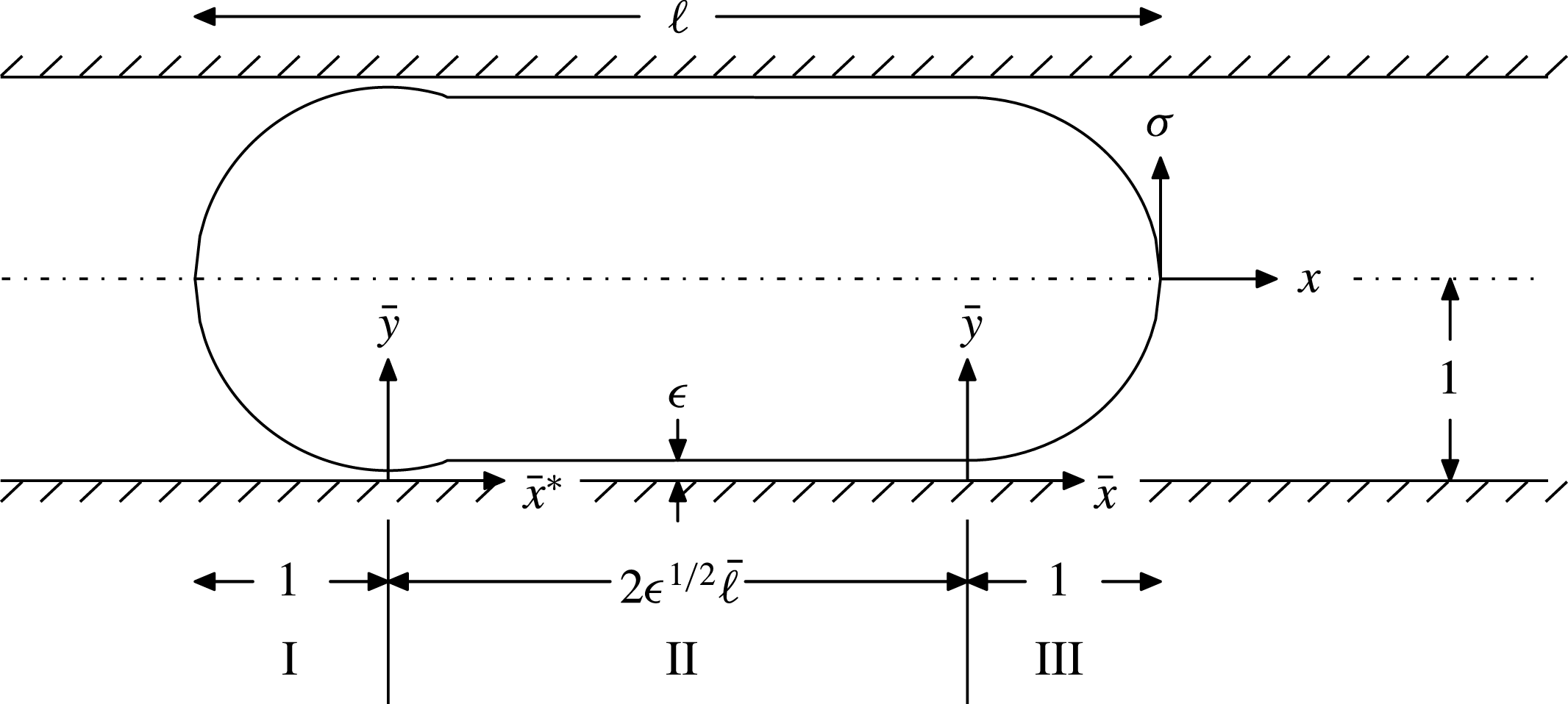
A schematic of the model problem is shown in figure 1. A vesicle is freely suspended in a bounded Poiseuille flow with mean speed
 $V$
and tube radius
 $R$
. The vesicle translates at a steady speed
 $U>V$
. In the moving reference frame, the vesicle appears stationary and the tube wall translates with velocity
 $-U$
. The fluids exterior and interior to the vesicle membrane are incompressible and Newtonian with shear viscosities
 $\unicode[STIX]{x1D707}$
and
 $\hat{\unicode[STIX]{x1D707}}$
, respectively. The membrane is taken to be an inextensible material surface with a bending stiffness
 $B$
. Axisymmetric cylindrical coordinates
 $(x,\unicode[STIX]{x1D70E},\unicode[STIX]{x1D719})$
are adopted with the origin placed at the tip of the front nose. The rear tail is located at
 $x=-L$
, where
 $L$
is the vesicle length. The gap between the vesicle membrane and the tube wall has a thickness
 $h^{\circ }$
at
 $x=-L/2$
. The shape of the membrane, which is unknown a priori, is described by the equation
 $$\begin{eqnarray}\unicode[STIX]{x1D70E}=r(x)=R-h(x),\end{eqnarray}$$
where
 $r(x)$
is the azimuthal radius of curvature and
 $h(x)$
is the gap height.
Schematic of a closely fitting, freely suspended vesicle translating in a circular tube. The system is rotationally symmetric about the
 $x$
-axis.

The velocity vector
 $\boldsymbol{u}$
and stress tensor
 $\unicode[STIX]{x1D64E}$
in the exterior fluid are represented in the axisymmetric cylindrical basis
 $(\boldsymbol{e}_{x},\boldsymbol{e}_{\unicode[STIX]{x1D70E}},\boldsymbol{e}_{\unicode[STIX]{x1D719}})$
as
 $$\begin{eqnarray}\boldsymbol{u}=u\boldsymbol{e}_{x}+v\boldsymbol{e}_{\unicode[STIX]{x1D70E}},\end{eqnarray}$$
 $$\begin{eqnarray}\displaystyle \unicode[STIX]{x1D64E} & = & \displaystyle \left(-p+2\unicode[STIX]{x1D707}\frac{\unicode[STIX]{x2202}u}{\unicode[STIX]{x2202}x}\right)\boldsymbol{e}_{x}\boldsymbol{e}_{x}+\left(-p+2\unicode[STIX]{x1D707}\frac{\unicode[STIX]{x2202}v}{\unicode[STIX]{x2202}\unicode[STIX]{x1D70E}}\right)\boldsymbol{e}_{\unicode[STIX]{x1D70E}}\boldsymbol{e}_{\unicode[STIX]{x1D70E}}+\left(-p+\frac{2\unicode[STIX]{x1D707}v}{\unicode[STIX]{x1D70E}}\right)\boldsymbol{e}_{\unicode[STIX]{x1D719}}\boldsymbol{e}_{\unicode[STIX]{x1D719}}\nonumber\\ \displaystyle & & \displaystyle +\,\unicode[STIX]{x1D707}\left(\frac{\unicode[STIX]{x2202}u}{\unicode[STIX]{x2202}\unicode[STIX]{x1D70E}}+\frac{\unicode[STIX]{x2202}v}{\unicode[STIX]{x2202}x}\right)(\boldsymbol{e}_{x}\boldsymbol{e}_{\unicode[STIX]{x1D70E}}+\boldsymbol{e}_{\unicode[STIX]{x1D70E}}\boldsymbol{e}_{x}),\end{eqnarray}$$
where
 $u(x,\unicode[STIX]{x1D70E})$
,
 $v(x,\unicode[STIX]{x1D70E})$
are the velocity components and
 $p(x,\unicode[STIX]{x1D70E})$
is the fluid pressure. The interior velocity
 $\hat{\boldsymbol{u}}$
and stress
 $\hat{\unicode[STIX]{x1D64E}}$
are given by similar expressions. In the creeping-flow regime, the steady equations and boundary conditions for the velocity and stress fields are as follows:
 $$\begin{eqnarray}\displaystyle & \displaystyle \left.\begin{array}{@{}l@{}}\unicode[STIX]{x1D735}\boldsymbol{\cdot }\boldsymbol{u}=0,\\ \unicode[STIX]{x1D735}\boldsymbol{\cdot }\unicode[STIX]{x1D64E}=-\unicode[STIX]{x1D735}p+\unicode[STIX]{x1D707}\unicode[STIX]{x1D6FB}^{2}\boldsymbol{u}=\mathbf{0},\end{array}\right\} & \displaystyle\end{eqnarray}$$
 $$\begin{eqnarray}\displaystyle & \displaystyle \left.\begin{array}{@{}l@{}}\unicode[STIX]{x1D735}\boldsymbol{\cdot }\hat{\boldsymbol{u}}=0,\\ \unicode[STIX]{x1D735}\boldsymbol{\cdot }\hat{\unicode[STIX]{x1D64E}}=-\unicode[STIX]{x1D735}\hat{p}+\hat{\unicode[STIX]{x1D707}}\unicode[STIX]{x1D6FB}^{2}\hat{\boldsymbol{u}}=\mathbf{0},\end{array}\right\} & \displaystyle\end{eqnarray}$$
 $$\begin{eqnarray}\displaystyle & \displaystyle \text{as }x\rightarrow \pm \infty :\qquad \boldsymbol{u}\rightarrow \left[2V\left(1-\frac{\unicode[STIX]{x1D70E}^{2}}{R^{2}}\right)-U\right]\boldsymbol{e}_{x}, & \displaystyle\end{eqnarray}$$
 $$\begin{eqnarray}\displaystyle & \displaystyle \text{at }\unicode[STIX]{x1D70E}=R:\qquad \boldsymbol{u}=-U\boldsymbol{e}_{x}, & \displaystyle\end{eqnarray}$$
 $$\begin{eqnarray}\displaystyle & \displaystyle \text{at }\unicode[STIX]{x1D70E}=0:\qquad \frac{\unicode[STIX]{x2202}u}{\unicode[STIX]{x2202}\unicode[STIX]{x1D70E}}=\frac{\unicode[STIX]{x2202}\hat{u} }{\unicode[STIX]{x2202}\unicode[STIX]{x1D70E}}=0,\quad v=\hat{v}=0, & \displaystyle\end{eqnarray}$$
 $$\begin{eqnarray}\displaystyle & \displaystyle \text{at }\unicode[STIX]{x1D70E}=r(x):\quad \boldsymbol{u}=\hat{\boldsymbol{u}}=\mathbf{0}, & \displaystyle\end{eqnarray}$$
 $$\begin{eqnarray}\displaystyle & & \displaystyle \text{at }\unicode[STIX]{x1D70E}=r(x):\qquad \boldsymbol{n}\boldsymbol{\cdot }(\unicode[STIX]{x1D64E}-\hat{\unicode[STIX]{x1D64E}})\boldsymbol{\cdot }\boldsymbol{n}\nonumber\\ \displaystyle & & \displaystyle \hspace{90.00014pt}=\unicode[STIX]{x1D70F}(\unicode[STIX]{x1D735}_{s}\boldsymbol{\cdot }\boldsymbol{n})-B[\unicode[STIX]{x1D735}_{s}\boldsymbol{n}\boldsymbol{ : }\unicode[STIX]{x1D735}_{s}\boldsymbol{n}-{\textstyle \frac{1}{2}}(\unicode[STIX]{x1D735}_{s}\boldsymbol{\cdot }\boldsymbol{n})^{2}+\unicode[STIX]{x1D6FB}_{s}^{2}](\unicode[STIX]{x1D735}_{s}\boldsymbol{\cdot }\boldsymbol{n}),\nonumber\\ \displaystyle & & \displaystyle\end{eqnarray}$$
 $$\begin{eqnarray}\displaystyle & & \displaystyle \text{at }\unicode[STIX]{x1D70E}=r(x):\qquad \unicode[STIX]{x1D644}_{s}\boldsymbol{\cdot }(\unicode[STIX]{x1D64E}-\hat{\unicode[STIX]{x1D64E}})\boldsymbol{\cdot }\boldsymbol{n}=-\unicode[STIX]{x1D735}_{s}\unicode[STIX]{x1D70F}.\end{eqnarray}$$
 $\boldsymbol{n}$
is the (outward pointing) unit normal of the vesicle surface,
 $\unicode[STIX]{x1D644}_{s}=\unicode[STIX]{x1D644}-\boldsymbol{n}\boldsymbol{n}$
is the surface unit tensor,
 $\unicode[STIX]{x1D735}_{s}=\unicode[STIX]{x1D644}_{s}\boldsymbol{\cdot }\unicode[STIX]{x1D735}$
is the surface gradient operator and
 $\unicode[STIX]{x1D70F}(x)$
is the membrane tension. The stress conditions (2.9) were derived by Jenkins (Reference Jenkins1977) and later by Zhong-can & Helfrich (Reference Zhong-can and Helfrich1989) using the principle of virtual work. In contrast to a bubble, for which the surface tension is taken to be a material property, the membrane tension
 $\unicode[STIX]{x1D70F}(x)$
is a field that enforces surface area incompressibility. In this sense,
 $\unicode[STIX]{x1D70F}(x)$
is analogous to a ‘two-dimensional pressure’ – the pressures
 $p(x,\unicode[STIX]{x1D70E})$
and
 $\hat{p}(x,\unicode[STIX]{x1D70E})$
enforce volume incompressibility in the bulk fluids. Surface area incompressibility for an axisymmetric, steady surface is enforced by (2.8).
The vesicle surface is a free boundary whose radius
 $r(x)$
is determined by (2.9a
). The boundary conditions for
 $r(x)$
are
 $$\begin{eqnarray}\displaystyle & \displaystyle \text{at }x=0:\qquad r=0,\quad \frac{\text{d}r}{\text{d}x}\rightarrow -\infty , & \displaystyle\end{eqnarray}$$
 $$\begin{eqnarray}\displaystyle & \displaystyle \text{at }x=-{\textstyle \frac{1}{2}}L:\qquad r=R-h^{\circ }, & \displaystyle\end{eqnarray}$$
 $$\begin{eqnarray}\displaystyle & \displaystyle \text{at }x=-L:\qquad r=0,\quad \frac{\text{d}r}{\text{d}x}\rightarrow \infty . & \displaystyle\end{eqnarray}$$
The ‘gap condition’, equation (2.11), appears to be ad hoc in the sense that the characteristic thickness
 $h^{\circ }$
is not typically controlled in a physical setting. However, this boundary condition greatly facilitates the forthcoming ‘narrow-gap assumption’ in § 4. It will prove useful, after a solution to the boundary-value problem is determined, to reparametrize the solution for fixed vesicle surface area
 $A$
and enclosed volume
 $\unicode[STIX]{x1D6FA}$
. These parameters are related to
 $r(x)$
by the integral relations,
 $$\begin{eqnarray}\displaystyle & \displaystyle A=\iint _{\unicode[STIX]{x2202}\unicode[STIX]{x1D6FA}}\boldsymbol{n}\boldsymbol{\cdot }\text{d}\boldsymbol{A}=\int _{-L}^{0}2\unicode[STIX]{x03C0}r\sqrt{1+\left(\frac{\text{d}r}{\text{d}x}\right)^{2}}\,\text{d}x, & \displaystyle\end{eqnarray}$$
 $$\begin{eqnarray}\displaystyle & \displaystyle \unicode[STIX]{x1D6FA}=\iiint _{\unicode[STIX]{x1D6FA}}\text{d}^{3}\boldsymbol{x}=\int _{-L}^{0}\unicode[STIX]{x03C0}r^{2}\,\text{d}x. & \displaystyle\end{eqnarray}$$
The vesicle mobility and wall resistance are derived by applying mass and force balances to the system. A mass balance gives
 $$\begin{eqnarray}\displaystyle & & \displaystyle \int _{0}^{2\unicode[STIX]{x03C0}}\int _{r(x)}^{R}u|_{x\in [-L,0]}\unicode[STIX]{x1D70E}\,\text{d}\unicode[STIX]{x1D70E}\,\text{d}\unicode[STIX]{x1D719}\nonumber\\ \displaystyle & & \displaystyle \quad =\int _{0}^{2\unicode[STIX]{x03C0}}\int _{0}^{R}u|_{|x|\rightarrow \infty }\unicode[STIX]{x1D70E}\,\text{d}\unicode[STIX]{x1D70E}\,\text{d}\unicode[STIX]{x1D719}=\unicode[STIX]{x03C0}R^{2}(V-U)\equiv -2\unicode[STIX]{x03C0}Rq,\end{eqnarray}$$
where
 $q$
is the leakback flux per unit circumference. At steady state, the vector flux
 $q\boldsymbol{e}_{x}$
is divergence free by the kinematic condition,
 $\text{d}q/\text{d}x=0$
. Applying a force balance gives
 $$\begin{eqnarray}2\unicode[STIX]{x03C0}R\int _{-\infty }^{\infty }\unicode[STIX]{x1D707}\left.\left(\frac{\unicode[STIX]{x2202}u}{\unicode[STIX]{x2202}\unicode[STIX]{x1D70E}}+\frac{\unicode[STIX]{x2202}v}{\unicode[STIX]{x2202}x}\right)\right|_{\unicode[STIX]{x1D70E}=R}\,\text{d}x=\unicode[STIX]{x03C0}R^{2}(p|_{x\rightarrow \infty }-p|_{x\rightarrow -\infty })\equiv -\unicode[STIX]{x03C0}R^{2}\unicode[STIX]{x0394}p,\end{eqnarray}$$
where
 $\unicode[STIX]{x0394}p$
is the pressure drop. The vector pressure drop
 $\unicode[STIX]{x0394}p\boldsymbol{e}_{x}$
balances the resultant of wall shear stresses, which diverges for an infinitely long tube. Equation (2.15) may be regularized by subtracting the Poiseuillean contribution
 $\int _{-\infty }^{\infty }(-8\unicode[STIX]{x03C0}\unicode[STIX]{x1D707}V)\,\text{d}x$
from both sides of the equation, leading to the definition of the extra pressure drop,
 $$\begin{eqnarray}\displaystyle \unicode[STIX]{x0394}p^{+} & \equiv & \displaystyle \unicode[STIX]{x0394}p-\frac{1}{\unicode[STIX]{x03C0}R^{2}}\int _{-\infty }^{\infty }8\unicode[STIX]{x03C0}\unicode[STIX]{x1D707}V\,\text{d}x\nonumber\\ \displaystyle & = & \displaystyle -\int _{-\infty }^{\infty }\left[\frac{2\unicode[STIX]{x1D707}}{R}\left(\frac{\unicode[STIX]{x2202}u}{\unicode[STIX]{x2202}\unicode[STIX]{x1D70E}}+\left.\frac{\unicode[STIX]{x2202}v}{\unicode[STIX]{x2202}x}\right)\right|_{\unicode[STIX]{x1D70E}=R}+\frac{8\unicode[STIX]{x1D707}V}{R^{2}}\right]\text{d}x,\end{eqnarray}$$
which is bounded.
Taken together, the preceding equations form a boundary-value problem for the velocity components
 $u$
,
 $v$
,
 $\hat{u}$
and
 $\hat{v}$
, pressures
 $p$
and
 $\hat{p}$
, membrane tension
 $\unicode[STIX]{x1D70F}$
, leakback flux
 $q$
, extra pressure drop
 $\unicode[STIX]{x0394}p^{+}$
and radius of curvature
 $r$
(or gap height
 $h$
). Although the governing equations of fluid flow (2.4) are linear, the free boundary problem is nonlinear due to the normal stress condition (2.9a
). The unknown fields are uniquely specified by fixing the fluid viscosities
 $\unicode[STIX]{x1D707}$
and
 $\hat{\unicode[STIX]{x1D707}}$
, membrane bending stiffness
 $B$
, vesicle length
 $L$
, gap height
 $h^{\circ }$
, tube radius
 $R$
and either the vesicle speed
 $U$
or the mean flow speed
 $V$
. The vesicle surface area
 $A$
and enclosed volume
 $\unicode[STIX]{x1D6FA}$
are determined incidentally.
3 Scalings and dimensionless groups
The basic equations may be put into dimensionless form upon selection of characteristic scales for the base units. Here, it is natural to use
 $R$
as a measure for distance,
 $R/U$
for time, and
 $\unicode[STIX]{x1D707}R^{2}/U$
for mass. Using these scales, the variables are rendered dimensionless as follows:
 $$\begin{eqnarray}\displaystyle & \displaystyle x,\unicode[STIX]{x1D70E},r,h\text{ are scaled by }R, & \displaystyle\end{eqnarray}$$
 $$\begin{eqnarray}\displaystyle & \displaystyle u,v,\hat{u} ,\hat{v}\text{ are scaled by }U, & \displaystyle\end{eqnarray}$$
 $$\begin{eqnarray}\displaystyle & \displaystyle p,\hat{p},\unicode[STIX]{x0394}p^{+}\text{ are scaled by }\unicode[STIX]{x1D707}U/R, & \displaystyle\end{eqnarray}$$
 $$\begin{eqnarray}\displaystyle & \displaystyle q\text{ is scaled by }UR, & \displaystyle\end{eqnarray}$$
 $$\begin{eqnarray}\displaystyle & \displaystyle \unicode[STIX]{x1D70F}\text{is scaled by }\unicode[STIX]{x1D707}U. & \displaystyle\end{eqnarray}$$
 $$\begin{eqnarray}\displaystyle & \displaystyle \unicode[STIX]{x1D705}=\frac{\hat{\unicode[STIX]{x1D707}}}{\unicode[STIX]{x1D707}}\text{ (the viscosity ratio),} & \displaystyle\end{eqnarray}$$
 $$\begin{eqnarray}\displaystyle & \displaystyle \unicode[STIX]{x1D6FD}=\frac{B}{\unicode[STIX]{x1D707}UR^{2}}\text{ (the bending parameter),} & \displaystyle\end{eqnarray}$$
 $$\begin{eqnarray}\displaystyle & \displaystyle \ell =\frac{L}{R}\text{ (the reduced length),} & \displaystyle\end{eqnarray}$$
 $$\begin{eqnarray}\displaystyle & \displaystyle \unicode[STIX]{x1D716}=\frac{h^{\circ }}{R}\text{ (the clearance parameter).} & \displaystyle\end{eqnarray}$$
 $\unicode[STIX]{x1D705}$
is a measure of the relative dissipation between the interior and exterior fluids. The bending parameter
 $\unicode[STIX]{x1D6FD}$
gauges the relative importance of membrane bending stiffness and viscous traction in the balance of normal stress on the membrane. (The reciprocal of
 $\unicode[STIX]{x1D6FD}$
is sometimes called the ‘capillary number’ in connection with vesicles. This terminology is avoided here because the capillary number is usually defined as the ratio of viscous stresses to surface tension stresses, the latter of which act to resist changes in surface area. Bending stresses act to resist changes in surface curvature, which is a fundamentally different effect.) The reduced length
 $\ell$
is the number of tube radii separating the front nose from the rear tail. Finally, the clearance parameter
 $\unicode[STIX]{x1D716}$
gives the fraction of the tube radius occupied by suspending fluid at the vesicle’s midplane.
At first glance, the choice of
 $\unicode[STIX]{x1D716}=h^{\circ }/R$
and
 $\ell =L/R$
as parameters may seem like an odd one. A more obvious choice would be something like
 $A/R^{2}$
and
 $\unicode[STIX]{x1D6FA}/R^{3}$
, which are purely geometric and independent of the flow conditions. However, parametrizing the boundary-value problem in terms of
 $\unicode[STIX]{x1D716}$
and
 $\ell$
is much more convenient when
 $\unicode[STIX]{x1D716}$
is small, as is assumed in § 4. Fortunately, this choice does not preclude utility of the theory. Once a solution is known, the parameters
 $\unicode[STIX]{x1D716}$
and
 $\ell$
may be eliminated in favour of purely geometric quantities – those that depend only on
 $A$
,
 $\unicode[STIX]{x1D6FA}$
and
 $R$
– with all of the dynamical information contained in
 $\unicode[STIX]{x1D6FD}$
. This process of elimination is carried out in § 8, after the main results are presented.
4 Narrow-gap assumption
 $(\unicode[STIX]{x1D716}\ll 1)$

The vesicle is assumed to be swollen to a near-critical volume, such that the clearance between the membrane and tube wall is small compared to unity,
 $$\begin{eqnarray}\unicode[STIX]{x1D716}\ll 1.\end{eqnarray}$$
Setting
 $\unicode[STIX]{x1D716}=0$
reduces the vesicle shape to a cylinder of length
 $\ell -2$
capped by two hemispheres of unit radius. For small (but non-vanishing) values of
 $\unicode[STIX]{x1D716}$
, a lubrication layer (the ‘inner region’) of length
 $\ell -2$
develops around the vesicle midsection. Within this lubrication layer,
 $h\ll 1$
and viscous shear stresses are amplified, which in turn drives large pressures. Outside this layer (the ‘outer region’), viscous stresses play a comparatively weaker role and the shape of the membrane is dictated by hydrostatics. This regional segregation of ‘dominant’ physical forces suggests that the limit
 $\unicode[STIX]{x1D716}\rightarrow 0$
is a singular one and, therefore, a perturbative solution ‘for small
 $\unicode[STIX]{x1D716}$
’ must be constructed by the method of matched asymptotic expansions.
A similar singular perturbation problem was investigated by Bretherton (Reference Bretherton1961) in analysing the motion of large bubbles of fixed volume translating through capillary tubes. In Bretherton’s theory, the small parameter
 $\unicode[STIX]{x1D716}$
was related to a balance between viscous stresses and surface tension – measured by the so-called ‘capillary number’. The membrane tension of a vesicle
 $\unicode[STIX]{x1D70F}(x)$
, which is a field that locally conserves surface area, is not analogous to the surface tension of a bubble, which is usually treated as a material property. Consequently, the small parameter
 $\unicode[STIX]{x1D716}$
cannot be directly connected with the balance between viscous stresses and surface relaxation. Rather,
 $\unicode[STIX]{x1D716}$
is geometrically constrained by fixing both the vesicle surface area and enclosed volume.
O’Neill & Stewartson (Reference O’Neill and Stewartson1967), in their study of spheres translating in the vicinity of planar boundaries, showed that the lateral and transverse length scales in the thin-film region must be stretched by
 $\unicode[STIX]{x1D716}^{1/2}$
and
 $\unicode[STIX]{x1D716}$
, respectively, in order for the particle surface to have contiguous curvature. Using the same arguments, the ‘inner coordinates’ in this work are defined as
 $$\begin{eqnarray}(\bar{x},\bar{x}^{\ast },\bar{y})=\left(\frac{x+1}{\unicode[STIX]{x1D716}^{1/2}},\frac{x+\ell -1}{\unicode[STIX]{x1D716}^{1/2}},\frac{1-\unicode[STIX]{x1D70E}}{\unicode[STIX]{x1D716}}\right),\end{eqnarray}$$
where an ‘overbar’ is used to denote a rescaling with respect to
 $\unicode[STIX]{x1D716}^{1/2}$
and an ‘asterisk’ is used to denote a shift of origin in the inner region. A schematic of the different regions and their associated coordinate systems is shown in figure 2. It is taken as an ansatz that
 $x=-1$
and
 $x=-\ell +1$
demarcate the ‘matching points’ separating the inner region from the outer regions. A more general formulation would leave the locations of the matching points as extra degrees of freedom to be determined as part of the solution (Park & Homsy Reference Park and Homsy1984).
The domain is divided into three regions: a ‘rear outer region’ (I), an ‘inner region’ (II) and a ‘front outer region’ (III). The inner coordinates
 $\bar{x}$
and
 $\bar{x}^{\ast }$
are related by a shift of origin,
 $\bar{x}^{\ast }=\bar{x}-2\bar{\ell }$
.

By stretching the coordinates according to (4.2) and requiring that the dependent variables balance in the governing equations, one deduces the following ‘stretched variables’:
 $$\begin{eqnarray}(\bar{u},\bar{v},\hat{\bar{u}},\hat{\bar{v}},\bar{p},\hat{\bar{p}},\bar{q},\bar{\unicode[STIX]{x1D70F}},\bar{h})=\left(u,-\frac{v}{\unicode[STIX]{x1D716}^{1/2}},\hat{u} ,\unicode[STIX]{x1D716}^{1/2}\hat{v},\unicode[STIX]{x1D716}^{3/2}p,\unicode[STIX]{x1D716}^{3/2}\hat{p},\frac{q}{\unicode[STIX]{x1D716}},\unicode[STIX]{x1D716}^{3/2}\unicode[STIX]{x1D70F},\frac{h}{\unicode[STIX]{x1D716}}\right).\end{eqnarray}$$
(The term ‘inner variable’ is avoided here, because in practice the variables may be stretched in either the outer or inner regions. The stretched pressures
 $\bar{p}$
and
 $\hat{\bar{p}}$
, for instance, are
 $O(1)$
in both regions.) The scalings for the transverse velocities
 $\bar{v}$
and
 $\hat{\bar{v}}$
are different because there is no need to rescale the transverse coordinate
 $\unicode[STIX]{x1D70E}$
in the interior fluid.
Finally, it is necessary to rescale the bending parameter
 $\unicode[STIX]{x1D6FD}$
and reduced length
 $\ell$
such that they are retained at leading order in the narrow-gap equations:
 $$\begin{eqnarray}(\bar{\unicode[STIX]{x1D6FD}},\bar{\ell })=\left(\unicode[STIX]{x1D716}^{1/2}\unicode[STIX]{x1D6FD},\frac{{\textstyle \frac{1}{2}}\ell -1}{\unicode[STIX]{x1D716}^{1/2}}\right).\end{eqnarray}$$
The viscosity ratio
 $\unicode[STIX]{x1D705}$
need not be rescaled. The rescaled bending parameter
 $\bar{\unicode[STIX]{x1D6FD}}$
represents the correct balance of bending and viscous stresses in the narrow-gap limit. The rescaled length
 $2\bar{\ell }$
is the axial distance (in inner coordinates) spanned by the lubricating film. In the following development, it is tacitly assumed that
 $$\begin{eqnarray}\unicode[STIX]{x1D705}=O(\unicode[STIX]{x1D716}^{-1/2})\quad \text{and}\quad \bar{\unicode[STIX]{x1D6FD}}=O(\unicode[STIX]{x1D716}^{-1/2}),\end{eqnarray}$$
so that the subsequent expansions are ‘uniformly asymptotic’.
In the next few subsections, the basic equations are rescaled and equations appropriate to the outer and inner regions are derived in light of the new scalings. Matching conditions at
 $x=-1$
and
 $x=-\ell +1$
will be presented thereafter.
4.1 Outer equations
In the outer region, the coordinates are not stretched and the velocity components need not be rescaled. The pressures
 $p(x,\unicode[STIX]{x1D70E})$
and
 $\hat{p}(x,\unicode[STIX]{x1D70E})$
and membrane tension
 $\unicode[STIX]{x1D70F}(x)$
must be stretched according to (4.3) in order to match consistently with the inner solution. The radius of curvature
 $r(x)$
, which spans the tube cross-section, is a suitable shape function for describing the membrane shape in the outer region.
The governing equations and boundary conditions for the outer region are as follows:
 $$\begin{eqnarray}\displaystyle & \displaystyle \frac{\unicode[STIX]{x2202}u}{\unicode[STIX]{x2202}x}+\left(\frac{\unicode[STIX]{x2202}}{\unicode[STIX]{x2202}\unicode[STIX]{x1D70E}}+\frac{1}{\unicode[STIX]{x1D70E}}\right)v=0, & \displaystyle\end{eqnarray}$$
 $$\begin{eqnarray}\displaystyle & \displaystyle \frac{\unicode[STIX]{x2202}\bar{p}}{\unicode[STIX]{x2202}x}-\unicode[STIX]{x1D716}^{3/2}\left(\frac{\unicode[STIX]{x2202}^{2}}{\unicode[STIX]{x2202}x^{2}}+\frac{\unicode[STIX]{x2202}^{2}}{\unicode[STIX]{x2202}\unicode[STIX]{x1D70E}^{2}}+\frac{1}{\unicode[STIX]{x1D70E}}\frac{\unicode[STIX]{x2202}}{\unicode[STIX]{x2202}\unicode[STIX]{x1D70E}}\right)u=0, & \displaystyle\end{eqnarray}$$
 $$\begin{eqnarray}\displaystyle & \displaystyle \frac{\unicode[STIX]{x2202}\bar{p}}{\unicode[STIX]{x2202}\unicode[STIX]{x1D70E}}-\unicode[STIX]{x1D716}^{3/2}\left(\frac{\unicode[STIX]{x2202}^{2}}{\unicode[STIX]{x2202}x^{2}}+\frac{\unicode[STIX]{x2202}^{2}}{\unicode[STIX]{x2202}\unicode[STIX]{x1D70E}^{2}}+\frac{1}{\unicode[STIX]{x1D70E}}\frac{\unicode[STIX]{x2202}}{\unicode[STIX]{x2202}\unicode[STIX]{x1D70E}}-\frac{1}{\unicode[STIX]{x1D70E}^{2}}\right)v=0, & \displaystyle\end{eqnarray}$$
 $$\begin{eqnarray}\displaystyle & \displaystyle \frac{\unicode[STIX]{x2202}\hat{u} }{\unicode[STIX]{x2202}x}+\left(\frac{\unicode[STIX]{x2202}}{\unicode[STIX]{x2202}\unicode[STIX]{x1D70E}}+\frac{1}{\unicode[STIX]{x1D70E}}\right)v=0, & \displaystyle\end{eqnarray}$$
 $$\begin{eqnarray}\displaystyle & \displaystyle \frac{\unicode[STIX]{x2202}\hat{\bar{p}}}{\unicode[STIX]{x2202}x}-\unicode[STIX]{x1D716}^{3/2}\unicode[STIX]{x1D705}\left(\frac{\unicode[STIX]{x2202}^{2}}{\unicode[STIX]{x2202}x^{2}}+\frac{\unicode[STIX]{x2202}^{2}}{\unicode[STIX]{x2202}\unicode[STIX]{x1D70E}^{2}}+\frac{1}{\unicode[STIX]{x1D70E}}\frac{\unicode[STIX]{x2202}}{\unicode[STIX]{x2202}\unicode[STIX]{x1D70E}}\right)\hat{u} =0, & \displaystyle\end{eqnarray}$$
 $$\begin{eqnarray}\displaystyle & \displaystyle \frac{\unicode[STIX]{x2202}\hat{\bar{p}}}{\unicode[STIX]{x2202}\unicode[STIX]{x1D70E}}-\unicode[STIX]{x1D716}^{3/2}\unicode[STIX]{x1D705}\left(\frac{\unicode[STIX]{x2202}^{2}}{\unicode[STIX]{x2202}x^{2}}+\frac{\unicode[STIX]{x2202}^{2}}{\unicode[STIX]{x2202}\unicode[STIX]{x1D70E}^{2}}+\frac{1}{\unicode[STIX]{x1D70E}}\frac{\unicode[STIX]{x2202}}{\unicode[STIX]{x2202}\unicode[STIX]{x1D70E}}-\frac{1}{\unicode[STIX]{x1D70E}^{2}}\right)\hat{v}=0, & \displaystyle\end{eqnarray}$$
 $$\begin{eqnarray}\displaystyle & \displaystyle \text{as }x\rightarrow \pm \infty :\qquad u\rightarrow \frac{2V}{U}(1-\unicode[STIX]{x1D70E}^{2})-1,\quad v=0, & \displaystyle\end{eqnarray}$$
 $$\begin{eqnarray}\displaystyle & \displaystyle \text{at }\unicode[STIX]{x1D70E}=1:\qquad u=-1,\quad v=0, & \displaystyle\end{eqnarray}$$
 $$\begin{eqnarray}\displaystyle & \displaystyle \text{at }\unicode[STIX]{x1D70E}=r(x):\qquad u=0,\quad v=0, & \displaystyle\end{eqnarray}$$
 $$\begin{eqnarray}\displaystyle & \displaystyle \text{at }\unicode[STIX]{x1D70E}=0:\qquad \frac{\unicode[STIX]{x2202}\hat{u} }{\unicode[STIX]{x2202}\unicode[STIX]{x1D70E}}=0,\quad \hat{v}=0, & \displaystyle\end{eqnarray}$$
 $$\begin{eqnarray}\displaystyle & \displaystyle \text{at }\unicode[STIX]{x1D70E}=r(x):\qquad \hat{u} =0,\quad \hat{v}=0, & \displaystyle\end{eqnarray}$$
 $$\begin{eqnarray}\displaystyle & & \displaystyle \text{at }\unicode[STIX]{x1D70E}=r(x):\nonumber\\ \displaystyle & & \displaystyle \qquad \left\{-(\bar{p}-\hat{\bar{p}})+\frac{2\unicode[STIX]{x1D716}^{3/2}}{1+(\text{d}r/\text{d}x)^{2}}\left[\left(\frac{\unicode[STIX]{x2202}}{\unicode[STIX]{x2202}\unicode[STIX]{x1D70E}}-\frac{\text{d}r}{\text{d}x}\frac{\unicode[STIX]{x2202}}{\unicode[STIX]{x2202}x}\right)(v-\unicode[STIX]{x1D705}\hat{v})\right.\right.\nonumber\\ \displaystyle & & \displaystyle \qquad \qquad -\left.\left.\frac{\text{d}r}{\text{d}x}\left(\frac{\unicode[STIX]{x2202}}{\unicode[STIX]{x2202}\unicode[STIX]{x1D70E}}-\frac{\text{d}r}{\text{d}x}\frac{\unicode[STIX]{x2202}}{\unicode[STIX]{x2202}x}\right)(u-\unicode[STIX]{x1D705}\hat{u} )\right]\right\}\nonumber\\ \displaystyle & & \displaystyle \qquad \quad =\bar{\unicode[STIX]{x1D70F}}\left(\frac{1}{r\sqrt{1+(\text{d}r/\text{d}x)^{2}}}-\frac{\text{d}^{2}r/\text{d}x^{2}}{\sqrt{1+(\text{d}r/\text{d}x)^{2}}^{3}}\right)\nonumber\\ \displaystyle & & \displaystyle \qquad \qquad +\,\unicode[STIX]{x1D716}\bar{\unicode[STIX]{x1D6FD}}\left\{\frac{1}{2}\left(\frac{1}{r\sqrt{1+(\text{d}r/\text{d}x)^{2}}}+\frac{\text{d}^{2}r/\text{d}x^{2}}{\sqrt{1+(\text{d}r/\text{d}x)^{2}}^{3}}\right)^{2}+\frac{1}{1+(\text{d}r/\text{d}x)^{2}}\frac{\text{d}^{2}}{\text{d}x^{2}}\right.\nonumber\\ \displaystyle & & \displaystyle \qquad \qquad -\,\left.\frac{1}{\sqrt{1+(\text{d}r/\text{d}x)^{2}}}\frac{\text{d}r}{\text{d}x}\left(-\frac{1}{r\sqrt{1+(\text{d}r/\text{d}x)^{2}}}+\frac{\text{d}^{2}r/\text{d}x^{2}}{\sqrt{1+(\text{d}r/\text{d}x)^{2}}^{3}}\right)\frac{\text{d}}{\text{d}x}\right\}\nonumber\\ \displaystyle & & \displaystyle \qquad \qquad \times \,\left(-\frac{1}{r\sqrt{1+(\text{d}r/\text{d}x)^{2}}}+\frac{\text{d}^{2}r/\text{d}x^{2}}{\sqrt{1+(\text{d}r/\text{d}x)^{2}}^{3}}\right),\end{eqnarray}$$
 $$\begin{eqnarray}\displaystyle & & \displaystyle \text{at }\unicode[STIX]{x1D70E}=r(x):\nonumber\\ \displaystyle & & \displaystyle \quad \frac{1}{\sqrt{1+(\text{d}r/\text{d}x)^{2}}}\frac{\text{d}\bar{\unicode[STIX]{x1D70F}}}{\text{d}x}+\frac{2\unicode[STIX]{x1D716}^{3/2}}{1+(\text{d}r/\text{d}x)^{2}}\left(\left\{\frac{\text{d}r}{\text{d}x}\frac{\unicode[STIX]{x2202}}{\unicode[STIX]{x2202}\unicode[STIX]{x1D70E}}+\left[1-\left(\frac{\text{d}r}{\text{d}x}\right)^{2}\right]\frac{\unicode[STIX]{x2202}}{\unicode[STIX]{x2202}x}\right\}(v-\unicode[STIX]{x1D705}\hat{v})\right.\nonumber\\ \displaystyle & & \displaystyle \qquad \quad -\,\left.\left\{\frac{\text{d}r}{\text{d}x}\frac{\unicode[STIX]{x2202}}{\unicode[STIX]{x2202}x}-\left[1-\left(\frac{\text{d}r}{\text{d}x}\right)^{2}\right]\frac{\unicode[STIX]{x2202}}{\unicode[STIX]{x2202}\unicode[STIX]{x1D70E}}\right\}(u-\unicode[STIX]{x1D705}\hat{u} )\right)=0,\end{eqnarray}$$
 $$\begin{eqnarray}\displaystyle & \displaystyle \text{at }x=0:\qquad r=0,\quad \frac{\text{d}r}{\text{d}x}\rightarrow -\infty , & \displaystyle\end{eqnarray}$$
 $$\begin{eqnarray}\displaystyle & \displaystyle \text{at }x=-\ell :\qquad r=0,\quad \frac{\text{d}r}{\text{d}x}\rightarrow \infty . & \displaystyle\end{eqnarray}$$
Equations (2.14) and (2.16) are not presented for the outer problem. The leakback flux
 $q$
and extra pressure drop
 $\unicode[STIX]{x0394}p^{+}$
may be uniquely determined from the inner equations, which are presented in the next section.
4.2 Inner equations
The variables in the inner region are stretched according to the definitions in (4.2)–(4.4). The radius of curvature
 $r(x)$
is replaced by the scaled gap thickness
 $\bar{h}(\bar{x})$
, which is a more suitable choice of shape function in the inner region. Since the governing equations are autonomous, it is understood that derivatives with respect to
 $\bar{x}$
may equivalently be written with respect to
 $\bar{x}^{\ast }$
. In the development of the inner equations, only terms up to
 $O(\unicode[STIX]{x1D716},\unicode[STIX]{x1D716}\unicode[STIX]{x1D705},\unicode[STIX]{x1D716}\bar{\unicode[STIX]{x1D6FD}})$
are retained.
The governing equations and boundary conditions for the inner region are as follows:
 $$\begin{eqnarray}\displaystyle & \displaystyle \frac{\unicode[STIX]{x2202}\bar{u}}{\unicode[STIX]{x2202}\bar{x}}+\left(\frac{\unicode[STIX]{x2202}}{\unicode[STIX]{x2202}\bar{y}}-\unicode[STIX]{x1D716}\right)\bar{v}=O(\unicode[STIX]{x1D716}^{2}), & \displaystyle\end{eqnarray}$$
 $$\begin{eqnarray}\displaystyle & \displaystyle \frac{\unicode[STIX]{x2202}\bar{p}}{\unicode[STIX]{x2202}\bar{x}}-\left[\frac{\unicode[STIX]{x2202}^{2}}{\unicode[STIX]{x2202}\bar{y}^{2}}+\unicode[STIX]{x1D716}\left(\frac{\unicode[STIX]{x2202}^{2}}{\unicode[STIX]{x2202}\bar{x}^{2}}-\frac{\unicode[STIX]{x2202}}{\unicode[STIX]{x2202}\bar{y}}\right)\right]\bar{u}=O(\unicode[STIX]{x1D716}^{2}), & \displaystyle\end{eqnarray}$$
 $$\begin{eqnarray}\displaystyle & \displaystyle \frac{\unicode[STIX]{x2202}\bar{p}}{\unicode[STIX]{x2202}\bar{y}}-\unicode[STIX]{x1D716}\frac{\unicode[STIX]{x2202}^{2}\bar{v}}{\unicode[STIX]{x2202}\bar{y}^{2}}=O(\unicode[STIX]{x1D716}^{2}), & \displaystyle\end{eqnarray}$$
 $$\begin{eqnarray}\displaystyle & \displaystyle \frac{\unicode[STIX]{x2202}\hat{\bar{u}}}{\unicode[STIX]{x2202}\bar{x}}+\left(\frac{\unicode[STIX]{x2202}}{\unicode[STIX]{x2202}\unicode[STIX]{x1D70E}}+\frac{1}{\unicode[STIX]{x1D70E}}\right)\hat{\bar{v}}=0, & \displaystyle\end{eqnarray}$$
 $$\begin{eqnarray}\displaystyle & \displaystyle \frac{\unicode[STIX]{x2202}\hat{\bar{p}}}{\unicode[STIX]{x2202}\bar{x}}-\unicode[STIX]{x1D716}\unicode[STIX]{x1D705}\frac{\unicode[STIX]{x2202}^{2}\hat{\bar{u}}}{\unicode[STIX]{x2202}\bar{x}^{2}}=O(\unicode[STIX]{x1D716}^{2}\unicode[STIX]{x1D705}), & \displaystyle\end{eqnarray}$$
 $$\begin{eqnarray}\displaystyle & \displaystyle \frac{\unicode[STIX]{x2202}\hat{\bar{p}}}{\unicode[STIX]{x2202}\unicode[STIX]{x1D70E}}-\unicode[STIX]{x1D705}\left[\frac{\unicode[STIX]{x2202}^{2}}{\unicode[STIX]{x2202}\bar{x}^{2}}+\unicode[STIX]{x1D716}\left(\frac{\unicode[STIX]{x2202}^{2}}{\unicode[STIX]{x2202}\unicode[STIX]{x1D70E}^{2}}+\frac{1}{\unicode[STIX]{x1D70E}}\frac{\unicode[STIX]{x2202}}{\unicode[STIX]{x2202}\unicode[STIX]{x1D70E}}-\frac{1}{\unicode[STIX]{x1D70E}^{2}}\right)\right]\hat{\bar{v}}=O(\unicode[STIX]{x1D716}^{2}\unicode[STIX]{x1D705}), & \displaystyle\end{eqnarray}$$
 $$\begin{eqnarray}\displaystyle & \displaystyle \text{at }\bar{y}=0:\qquad \bar{u}=-1,\quad \bar{v}=0, & \displaystyle\end{eqnarray}$$
 $$\begin{eqnarray}\displaystyle & \displaystyle \text{at }\bar{y}=\bar{h}(\bar{x}):\qquad \bar{u}=0,\bar{v}=0, & \displaystyle\end{eqnarray}$$
 $$\begin{eqnarray}\displaystyle & \displaystyle \text{at }\unicode[STIX]{x1D70E}=0:\qquad \frac{\unicode[STIX]{x2202}\hat{\bar{u}}}{\unicode[STIX]{x2202}\unicode[STIX]{x1D70E}}=0,\quad \hat{\bar{v}}=0, & \displaystyle\end{eqnarray}$$
 $$\begin{eqnarray}\displaystyle & \displaystyle \text{at }\unicode[STIX]{x1D70E}=1-\unicode[STIX]{x1D716}\bar{h}(\bar{x}):\qquad \hat{\bar{u}}=0,\quad \hat{\bar{v}}=0, & \displaystyle\end{eqnarray}$$
 $$\begin{eqnarray}\displaystyle & & \displaystyle \text{at }\bar{y}=\bar{h}(\bar{x}),\unicode[STIX]{x1D70E}=1-\unicode[STIX]{x1D716}\bar{h}(\bar{x}):\nonumber\\ \displaystyle & & \displaystyle \quad -(\bar{p}-\hat{\bar{p}})+2\unicode[STIX]{x1D716}\left[\frac{\unicode[STIX]{x2202}\bar{v}}{\unicode[STIX]{x2202}\bar{y}}-\frac{\text{d}\bar{h}}{\text{d}\bar{x}}\frac{\unicode[STIX]{x2202}\bar{u}}{\unicode[STIX]{x2202}\bar{y}}-\unicode[STIX]{x1D705}\left(\frac{\unicode[STIX]{x2202}}{\unicode[STIX]{x2202}\unicode[STIX]{x1D70E}}+\frac{\text{d}\bar{h}}{\text{d}\bar{x}}\frac{\unicode[STIX]{x2202}}{\unicode[STIX]{x2202}\bar{x}}\right)\hat{\bar{v}}\right]\nonumber\\ \displaystyle & & \displaystyle \qquad \quad =\bar{\unicode[STIX]{x1D70F}}\left\{\left(1+\frac{\text{d}^{2}\bar{h}}{\text{d}\bar{x}^{2}}\right)+\unicode[STIX]{x1D716}\left[\bar{h}-\frac{1}{2}\left(\frac{\text{d}\bar{h}}{\text{d}\bar{x}}\right)^{2}\left(1+3\frac{\text{d}^{2}\bar{h}}{\text{d}\bar{x}^{2}}\right)\right]\right\}\nonumber\\ \displaystyle & & \displaystyle \qquad \qquad -\,\bar{\unicode[STIX]{x1D6FD}}\left\{\frac{\text{d}^{4}\bar{h}}{\text{d}\bar{x}^{4}}+\unicode[STIX]{x1D716}\left[\frac{1}{2}\left(1+\frac{\text{d}^{2}\bar{h}}{\text{d}\bar{x}^{2}}\right)-\frac{3}{2}\left(\frac{\text{d}^{2}\bar{h}}{\text{d}\bar{x}^{2}}\right)^{2}-2\frac{\text{d}\bar{h}}{\text{d}\bar{x}}\frac{\text{d}^{3}\bar{h}}{\text{d}\bar{x}^{3}}-\frac{5}{2}\left(\frac{\text{d}^{2}\bar{h}}{\text{d}\bar{x}^{2}}\right)^{3}\right.\right.\nonumber\\ \displaystyle & & \displaystyle \qquad \qquad -\left.\left.10\frac{\text{d}\bar{h}}{\text{d}\bar{x}}\frac{\text{d}^{2}\bar{h}}{\text{d}\bar{x}^{2}}\frac{\text{d}^{3}\bar{h}}{\text{d}\bar{x}^{3}}-\frac{5}{2}\left(\frac{\text{d}\bar{h}}{\text{d}\bar{x}}\right)^{2}\frac{\text{d}^{4}\bar{h}}{\text{d}\bar{x}^{4}}\right]\right\}+O(\unicode[STIX]{x1D716}^{2}\bar{\unicode[STIX]{x1D6FD}},\unicode[STIX]{x1D716}^{2},\unicode[STIX]{x1D716}^{2}\unicode[STIX]{x1D705}),\end{eqnarray}$$
 $$\begin{eqnarray}\displaystyle & \displaystyle \text{at }\bar{y}=\bar{h}(\bar{x}),\unicode[STIX]{x1D70E}=1-\unicode[STIX]{x1D716}\bar{h}(\bar{x}):\qquad \frac{\text{d}\bar{\unicode[STIX]{x1D70F}}}{\text{d}\bar{x}}-\unicode[STIX]{x1D716}\frac{\unicode[STIX]{x2202}\bar{u}}{\unicode[STIX]{x2202}\bar{y}}-\unicode[STIX]{x1D716}\unicode[STIX]{x1D705}\frac{\unicode[STIX]{x2202}\hat{\bar{v}}}{\unicode[STIX]{x2202}\bar{x}}=O(\unicode[STIX]{x1D716}^{2},\unicode[STIX]{x1D716}^{2}\unicode[STIX]{x1D705}), & \displaystyle\end{eqnarray}$$
 $$\begin{eqnarray}\displaystyle & \displaystyle \text{at }\bar{x}=-\bar{\ell },\bar{x}^{\ast }=\bar{\ell }:\qquad \bar{h}=1, & \displaystyle\end{eqnarray}$$
 $$\begin{eqnarray}\displaystyle & \displaystyle \bar{q}=-\int _{0}^{\bar{h}(\bar{x})}\bar{u}\,(1-\unicode[STIX]{x1D716}\bar{y})\,\text{d}\bar{y}=\text{const.}, & \displaystyle\end{eqnarray}$$
 $$\begin{eqnarray}\displaystyle & \displaystyle \unicode[STIX]{x0394}\bar{p}^{+}=2\unicode[STIX]{x1D716}\left.\int _{-\infty }^{\bar{\ell }}\frac{\unicode[STIX]{x2202}\bar{u}}{\unicode[STIX]{x2202}\bar{y}}\right|_{\bar{y}=0}\,\text{d}\bar{x}^{\ast }+2\unicode[STIX]{x1D716}\left.\int _{-\bar{\ell }}^{\infty }\frac{\unicode[STIX]{x2202}\bar{u}}{\unicode[STIX]{x2202}\bar{y}}\right|_{\bar{y}=0}\,\text{d}\bar{x}+O(\unicode[STIX]{x1D716}^{3/2})=\text{const}. & \displaystyle\end{eqnarray}$$
To leading order, the leakback flux
 $\bar{q}$
and extra pressure drop
 $\unicode[STIX]{x0394}\bar{p}^{+}$
are determined entirely from the inner solution. The error term omitted in (4.27) contains higher-order contributions from the inner region as well as the leading-order contribution from the outer region.
4.3 Matching conditions
The foregoing equations are valid in the outer and inner regions separately. In order to unify the solutions, matching conditions must be developed at the matching points
 $x=-1$
and
 $-\ell +1$
. Of particular importance are the matching conditions for the membrane shape:
 $$\begin{eqnarray}\lim _{x\rightarrow -1}1-r(x)=\lim _{\bar{x}\rightarrow \infty }\unicode[STIX]{x1D716}\bar{h}(\bar{x})\end{eqnarray}$$
at the front nose and
 $$\begin{eqnarray}\lim _{x\rightarrow -\ell +1}1-r(x)=\lim _{\bar{x}^{\ast }\rightarrow -\infty }\unicode[STIX]{x1D716}\bar{h}(\bar{x})\end{eqnarray}$$
at the rear tail. The limits are interpreted in the spirit of the matching principle of van Dyke (Reference van Dyke1964). With the inclusion of these matching conditions, the boundary-value problem is well posed.
5 Small-
$\unicode[STIX]{x1D716}$
expansion

Rather than solve for the unknown variables using methods for partial differential equations, the variables are expanded in power series with respect to
 $\unicode[STIX]{x1D716}^{1/2}$
, viz.
 $$\begin{eqnarray}\unicode[STIX]{x1D713}(x,\unicode[STIX]{x1D70E})=\unicode[STIX]{x1D713}_{0}(x,\unicode[STIX]{x1D70E})+\unicode[STIX]{x1D716}^{1/2}\unicode[STIX]{x1D713}_{1}(x,\unicode[STIX]{x1D70E})+\unicode[STIX]{x1D716}\unicode[STIX]{x1D713}_{2}(x,\unicode[STIX]{x1D70E})+\cdots\end{eqnarray}$$
for the generic ‘unstretched’ variable
 $\unicode[STIX]{x1D713}$
and
 $$\begin{eqnarray}\bar{\unicode[STIX]{x1D713}}(\bar{x},\bar{y})=\bar{\unicode[STIX]{x1D713}}_{0}(\bar{x},\bar{y})+\unicode[STIX]{x1D716}^{1/2}\bar{\unicode[STIX]{x1D713}}_{1}(\bar{x},\bar{y})+\unicode[STIX]{x1D716}\bar{\unicode[STIX]{x1D713}}_{2}(\bar{x},\bar{y})+\cdots\end{eqnarray}$$
for the generic ‘stretched’ variable
 $\bar{\unicode[STIX]{x1D713}}$
. By expanding the dependent variables in powers of
 $\unicode[STIX]{x1D716}^{1/2}$
and collecting terms of like order in
 $\unicode[STIX]{x1D716}^{1/2}$
from the equations presented in § 4, an ordered set of perturbation equations is obtained. These equations are to be solved sequentially, beginning by setting
 $\unicode[STIX]{x1D716}=0$
so as to derive the so-called ‘leading-order solution’. Corrections to this solution are subsequently obtained by expanding the perturbation equations to higher order in
 $\unicode[STIX]{x1D716}^{1/2}$
.
The solution procedure begins in the outer region (§ 5.1), in which viscous stresses are relatively unimportant and the shape of the membrane is controlled by hydrostatics. In the inner region (§ 5.2), the fluid flow is governed by the equations of lubrication theory. The outer solution forces the inner solution through the matching conditions, which are applied as needed during the course of constructing the solutions. Higher-order corrections are evaluated in § 5.3.
5.1 Outer region
By expanding (4.6), (4.7) and (4.14) with respect to
 $\unicode[STIX]{x1D716}^{1/2}$
and setting
 $\unicode[STIX]{x1D716}=0$
, one immediately deduces that
 $\bar{p}_{0}$
,
 $\hat{\bar{p}}_{0}$
and
 $\bar{\unicode[STIX]{x1D70F}}_{0}$
are independent of spatial position. Thus, viscous stresses play no appreciable role in the outer region at this order. The leading-order problem reduces to the solution of the normal stress condition for the shape function
 $r_{0}(x)$
(cf. (4.13)),
 $$\begin{eqnarray}\bar{p}_{0}-\hat{\bar{p}}_{0}=-\bar{\unicode[STIX]{x1D70F}}_{0}\left(\frac{1}{r_{0}\sqrt{1+(\text{d}r_{0}/\text{d}x)^{2}}}-\frac{\text{d}^{2}r_{0}/\text{d}x^{2}}{\sqrt{1+(\text{d}r_{0}/\text{d}x)^{2}}^{3}}\right),\end{eqnarray}$$
with the boundary conditions (cf. (4.15)–(4.16) and (4.28)),
 $$\begin{eqnarray}\displaystyle & \displaystyle \text{at }x=0:\qquad r_{0}=0,\quad \frac{\text{d}r_{0}}{\text{d}x}\rightarrow -\infty , & \displaystyle\end{eqnarray}$$
 $$\begin{eqnarray}\displaystyle & \displaystyle \text{at }x=-\ell :\qquad r_{0}=0,\quad \frac{\text{d}r_{0}}{\text{d}x}\rightarrow \infty , & \displaystyle\end{eqnarray}$$
 $$\begin{eqnarray}\displaystyle & \displaystyle \text{at }x=-1,-\ell +1:\qquad r_{0}=1. & \displaystyle\end{eqnarray}$$
Although the fluid pressures and membrane tension do not vary in the outer region, there exists the possibility of a mismatch between their ‘front’ and ‘rear’ values as a result of variations through the inner region. Thus, it is in general necessary to determine the outer solutions at the front nose and rear tail independently of each other and unify them through the inner solution.
The solution of (5.3)–(5.6) is
 $$\begin{eqnarray}r_{0}=\sqrt{1-\unicode[STIX]{x1D709}^{2}},\quad \bar{p}_{0}-\hat{\bar{p}}_{0}=-2\bar{\unicode[STIX]{x1D70F}}_{0},\end{eqnarray}$$
where
 $$\begin{eqnarray}\unicode[STIX]{x1D709}=\left\{\begin{array}{@{}ll@{}}x+1,\quad & \text{for }x\in [-1,0],\\ x+\ell -1,\quad & \text{for }x\in [-\ell ,-\ell +1],\\ 0,\quad & \text{otherwise.}\end{array}\right.\end{eqnarray}$$
Thus, the leading-order vesicle shape is a spherocylinder (a cylinder capped by two hemispheres). The membrane tension
 $\bar{\unicode[STIX]{x1D70F}}_{0}$
remains unknown and must be determined from matching to the inner solution.
It happens that the
 $O(\unicode[STIX]{x1D716}^{1/2})$
correction to the shape function,
 $r_{1}(x)$
, may be determined without knowledge of the inner solution. The corrections
 $\bar{p}_{1}$
,
 $\hat{\bar{p}}_{1}$
and
 $\bar{\unicode[STIX]{x1D70F}}_{1}$
are spatially invariant, whence the
 $O(\unicode[STIX]{x1D716}^{1/2})$
term in (4.13) simplifies to
 $$\begin{eqnarray}\bar{p}_{1}-\hat{\bar{p}}_{1}=-2\bar{\unicode[STIX]{x1D70F}}_{1}+\bar{\unicode[STIX]{x1D70F}}_{0}\left(\frac{r_{1}}{r_{0}}-4r_{0}\sqrt{1-r_{0}^{2}}\frac{\text{d}r_{1}}{\text{d}x}+r_{0}^{3}\frac{\text{d}^{2}r_{1}}{\text{d}x^{2}}\right).\end{eqnarray}$$
With some rearrangement and introduction of the modified variables,
 $$\begin{eqnarray}f_{1}=r_{0}r_{1},\quad a_{1}=\frac{\bar{\unicode[STIX]{x1D70F}}_{1}}{\bar{\unicode[STIX]{x1D70F}}_{0}}-\frac{\bar{p}_{1}-\hat{\bar{p}}_{1}}{\bar{p}_{0}-\hat{\bar{p}}_{0}}=\text{const.},\end{eqnarray}$$
equation (5.9) may be recast as an inhomogeneous Legendre equation of order one,
 $$\begin{eqnarray}(1-\unicode[STIX]{x1D709}^{2})\frac{\text{d}^{2}f_{1}}{\text{d}\unicode[STIX]{x1D709}^{2}}-2\unicode[STIX]{x1D709}\frac{\text{d}f_{1}}{\text{d}\unicode[STIX]{x1D709}}+2f_{1}=2a_{1}.\end{eqnarray}$$
Here, the shifted coordinate
 $\unicode[STIX]{x1D709}$
is defined as before. The rear tail spans the region
 $\unicode[STIX]{x1D709}\in [-1,0]$
, while the front nose spans
 $\unicode[STIX]{x1D709}\in [0,1]$
. The boundary conditions for
 $f_{1}(\unicode[STIX]{x1D709})$
are
 $$\begin{eqnarray}\displaystyle & \displaystyle \text{at }\unicode[STIX]{x1D709}=0:\qquad f_{1}=0, & \displaystyle\end{eqnarray}$$
 $$\begin{eqnarray}\displaystyle & \displaystyle \text{at }\unicode[STIX]{x1D709}=\pm 1:\qquad f_{1}=0. & \displaystyle\end{eqnarray}$$
The only solution of (5.11) which satisfies (5.12)–(5.13) is the trivial solution,
 $$\begin{eqnarray}f_{1}=0,\quad a_{1}=0.\end{eqnarray}$$
Therefore,
 $$\begin{eqnarray}r_{1}=0,\quad \bar{p}_{1}-\hat{\bar{p}}_{1}=-2\bar{\unicode[STIX]{x1D70F}}_{1},\end{eqnarray}$$
i.e. the
 $O(\unicode[STIX]{x1D716}^{1/2})$
solution admits no correction to the shape. The membrane tension
 $\bar{\unicode[STIX]{x1D70F}}_{1}$
remains unknown and must be determined from matching to the inner solution.
5.2 Inner region
In contrast to the ‘static’ outer region, viscous stresses play a significant role in the inner region. The governing equations and boundary conditions are
 $$\begin{eqnarray}\frac{\unicode[STIX]{x2202}\bar{u}_{0}}{\unicode[STIX]{x2202}\bar{x}}+\frac{\unicode[STIX]{x2202}\bar{v}_{0}}{\unicode[STIX]{x2202}\bar{y}}=0,\quad \frac{\unicode[STIX]{x2202}\bar{p}_{0}}{\unicode[STIX]{x2202}\bar{x}}-\frac{\unicode[STIX]{x2202}^{2}\bar{u}_{0}}{\unicode[STIX]{x2202}\bar{y}^{2}}=0,\quad \frac{\unicode[STIX]{x2202}\bar{p}_{0}}{\unicode[STIX]{x2202}\bar{y}}=0,\end{eqnarray}$$
 $$\begin{eqnarray}\frac{\unicode[STIX]{x2202}\hat{\bar{u}}_{0}}{\unicode[STIX]{x2202}\bar{x}}+\left(\frac{\unicode[STIX]{x2202}}{\unicode[STIX]{x2202}\unicode[STIX]{x1D70E}}+\frac{1}{\unicode[STIX]{x1D70E}}\right)\hat{\bar{v}}_{0}=0,\quad \frac{\unicode[STIX]{x2202}\hat{\bar{p}}_{0}}{\unicode[STIX]{x2202}\bar{x}}=0,\quad \frac{\unicode[STIX]{x2202}\hat{\bar{p}}_{0}}{\unicode[STIX]{x2202}\unicode[STIX]{x1D70E}}-\unicode[STIX]{x1D705}\frac{\unicode[STIX]{x2202}^{2}\hat{\bar{v}}_{0}}{\unicode[STIX]{x2202}\bar{x}^{2}}=0,\end{eqnarray}$$
 $$\begin{eqnarray}\displaystyle & \displaystyle \text{at }\bar{y}=0:\qquad \bar{u}_{0}=-1,\quad \bar{v}_{0}=0, & \displaystyle\end{eqnarray}$$
 $$\begin{eqnarray}\displaystyle & \displaystyle \text{at }\bar{y}=\bar{h}_{0}(\bar{x}):\qquad \bar{u}_{0}=0,\quad \bar{v}_{0}=0, & \displaystyle\end{eqnarray}$$
 $$\begin{eqnarray}\displaystyle & \displaystyle \text{at }\unicode[STIX]{x1D70E}=0:\qquad \frac{\unicode[STIX]{x2202}\hat{\bar{u}}_{0}}{\unicode[STIX]{x2202}\unicode[STIX]{x1D70E}}=0,\quad \hat{\bar{v}}_{0}=0, & \displaystyle\end{eqnarray}$$
 $$\begin{eqnarray}\displaystyle & \displaystyle \text{at }\unicode[STIX]{x1D70E}=1:\qquad \hat{\bar{u}}_{0}=0,\quad \hat{\bar{v}}_{0}=0, & \displaystyle\end{eqnarray}$$
 $$\begin{eqnarray}\displaystyle & \displaystyle \text{at }\bar{y}=\bar{h}_{0}(\bar{x}):\qquad \bar{p}_{0}-\hat{\bar{p}}_{0}=-\bar{\unicode[STIX]{x1D70F}}_{0}\left(1+\frac{\text{d}^{2}\bar{h}_{0}}{\text{d}\bar{x}^{2}}\right)+\bar{\unicode[STIX]{x1D6FD}}\frac{\text{d}^{4}\bar{h}_{0}}{\text{d}\bar{x}^{4}},\quad \bar{\unicode[STIX]{x1D70F}}_{0}=\text{const.}, & \displaystyle\end{eqnarray}$$
 $$\begin{eqnarray}\displaystyle & \displaystyle \bar{q}_{0}=-\int _{0}^{\bar{h}_{0}(\bar{x})}\bar{u}_{0}\,\text{d}\bar{y}=\text{const.}, & \displaystyle\end{eqnarray}$$
 $$\begin{eqnarray}\displaystyle & \displaystyle \unicode[STIX]{x0394}\bar{p}_{2}^{+}=2\left.\int _{-\infty }^{\bar{\ell }}\frac{\unicode[STIX]{x2202}\bar{u}_{0}}{\unicode[STIX]{x2202}\bar{y}}\right|_{\bar{y}=0}\,\text{d}\bar{x}^{\ast }+2\left.\int _{-\bar{\ell }}^{\infty }\frac{\unicode[STIX]{x2202}\bar{u}_{0}}{\unicode[STIX]{x2202}\bar{y}}\right|_{\bar{y}=0}\,\text{d}\bar{x}=\text{const}. & \displaystyle\end{eqnarray}$$
Equations (5.16)–(5.21) and (5.23)–(5.24) are the equations of lubrication theory. Following Lighthill (Reference Lighthill1968), they may be used to derive the so-called ‘Reynolds equation’ for the pressure gradient,
 $$\begin{eqnarray}\frac{\text{d}\bar{p}_{0}}{\text{d}\bar{x}}=\frac{\text{d}(\bar{p}_{0}-\hat{\bar{p}}_{0})}{\text{d}\bar{x}}=-\frac{6}{\bar{h}_{0}^{2}}\left(1-\frac{2\bar{q}_{0}}{\bar{h}_{0}}\right),\end{eqnarray}$$
as well as an expression for the extra pressure drop,
 $$\begin{eqnarray}\unicode[STIX]{x0394}\bar{p}_{2}^{+}=\int _{-\infty }^{\bar{\ell }}\frac{4}{\bar{h}_{0}}\left(2-\frac{3\bar{q}_{0}}{\bar{h}_{0}}\right)\,\text{d}\bar{x}^{\ast }+\int _{-\bar{\ell }}^{\infty }\frac{4}{\bar{h}_{0}}\left(2-\frac{3\bar{q}_{0}}{\bar{h}_{0}}\right)\,\text{d}\bar{x}.\end{eqnarray}$$
The gap height
 $\bar{h}_{0}(\bar{x})$
remains to be determined. Combining the Reynolds equation (5.25) with the stress condition (5.22) leads to a differential equation for
 $\bar{h}_{0}(\bar{x})$
that bears some resemblance to the one originally considered by Landau & Levich (Reference Landau and Levich1942) (with the addition of the bending term):
 $$\begin{eqnarray}\bar{\unicode[STIX]{x1D6FD}}\frac{\text{d}^{5}\bar{h}_{0}}{\text{d}\bar{x}^{5}}-\bar{\unicode[STIX]{x1D70F}}_{0}\frac{\text{d}^{3}\bar{h}_{0}}{\text{d}\bar{x}^{3}}+\frac{6}{\bar{h}_{0}^{2}}\left(1-\frac{2\bar{q}_{0}}{\bar{h}_{0}}\right)=0.\end{eqnarray}$$
Dixit & Homsy (Reference Dixit and Homsy2013a ,Reference Dixit and Homsy b ) derived a similar expression to (5.27) for a stress-free interface in their study of particle-laden, dip-coating flow. The boundary conditions associated with equation (5.27) are as follows (cf. (4.25) and (4.28)):
 $$\begin{eqnarray}\displaystyle & \displaystyle \text{at }\bar{x}=-\bar{\ell },\bar{x}^{\ast }=\bar{\ell }:\qquad \bar{h}_{0}=1, & \displaystyle\end{eqnarray}$$
 $$\begin{eqnarray}\displaystyle & \displaystyle \text{as }\bar{x}\rightarrow \infty :\qquad \bar{h}_{0}\rightarrow b_{0}+{\textstyle \frac{1}{2}}\bar{x}^{2}, & \displaystyle\end{eqnarray}$$
 $$\begin{eqnarray}\displaystyle & \displaystyle \text{as }\bar{x}^{\ast }\rightarrow -\infty :\qquad \bar{h}_{0}\rightarrow b_{0}^{\ast }+{\textstyle \frac{1}{2}}\bar{x}^{\ast 2}, & \displaystyle\end{eqnarray}$$
where
 $$\begin{eqnarray}b_{0}=-r_{2}(-1),\quad b_{0}^{\ast }=-r_{2}(-\ell +1)\end{eqnarray}$$
are constants of integration. Since (5.27) is autonomous, it may be rewritten with
 $\bar{x}^{\ast }=\bar{x}-2\bar{\ell }$
substituted for
 $\bar{x}$
as the independent variable. Thus, matching with the ‘front’ and ‘rear’ outer solutions is facilitated by a simple shift of origin.
Equations (5.26)–(5.30) must be integrated numerically for specific values of the reduced length
 $\bar{\ell }$
and bending parameter
 $\bar{\unicode[STIX]{x1D6FD}}$
. The constants
 $\bar{q}_{0}$
,
 $\bar{\unicode[STIX]{x1D70F}}_{0}$
,
 $b_{0}$
,
 $b_{0}^{\ast }$
and
 $\unicode[STIX]{x0394}\bar{p}_{2}^{+}$
are determined simultaneously with
 $\bar{h}_{0}(\bar{x})$
during the integration procedure. Since the boundary-value problem is ill conditioned for many values of the parameters, the ‘multiple shooting method’ is employed for the numerical integration (Morrison, Riley & Zancanaro Reference Morrison, Riley and Zancanaro1962). A good description of the method is given in Stoer & Bulirsch (Reference Stoer and Bulirsch2002). In brief, the domain is first divided into two subdomains
 $\bar{x}\in [-\bar{\ell },\bar{X}]$
and
 $\bar{x}^{\ast }\in [-\bar{X}^{\ast },\bar{\ell }]$
. The boundary conditions are applied at
 $\bar{x}=\bar{X}$
,
 $\bar{x}=-\bar{\ell }$
,
 $\bar{x}^{\ast }=\bar{X}^{\ast }$
and
 $\bar{x}^{\ast }=\bar{\ell }$
. Care is taken to subtract off the error incurred by applying the far-field conditions (5.29)–(5.30) at finite boundaries
 $\bar{x}=\bar{X}$
and
 $\bar{x}=\bar{X}^{\ast }$
. Each subdomain is further divided into
 $O(10{-}100)$
segments separated by ‘shooting points’ at which continuity conditions are applied. Integration is carried out over each segment using a fourth-order Runge–Kutta scheme. Newton iteration with line search and backtracking is used to enforce the boundary and continuity conditions at the shooting points. The iteration is truncated when the norm of the subsequent Newton step or the norm of the function to be zeroed falls below
 $10^{-12}$
. In order to avoid numerical errors associated with the behaviour of the solution near the boundaries, integration always proceeds away from the boundary points towards a ‘fitting point’ located at the centre of the subdomain. Once a solution for particular values of
 $\bar{\ell }$
and
 $\bar{\unicode[STIX]{x1D6FD}}$
is known, additional solutions may be generated using the continuation method.
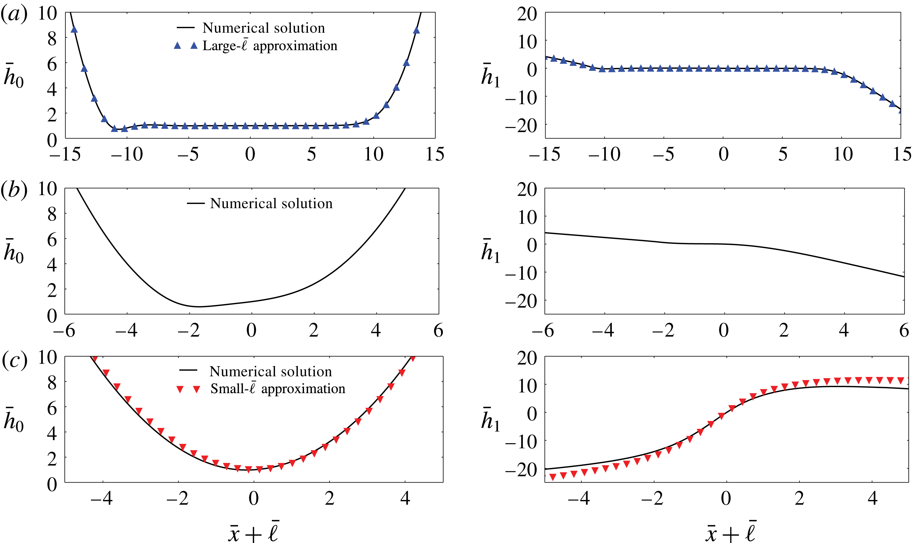
Representative profiles of
 $\bar{h}_{0}(\bar{x})$
are plotted in figure 3 for
 $\bar{\unicode[STIX]{x1D6FD}}=0$
and three different values of
 $\bar{\ell }$
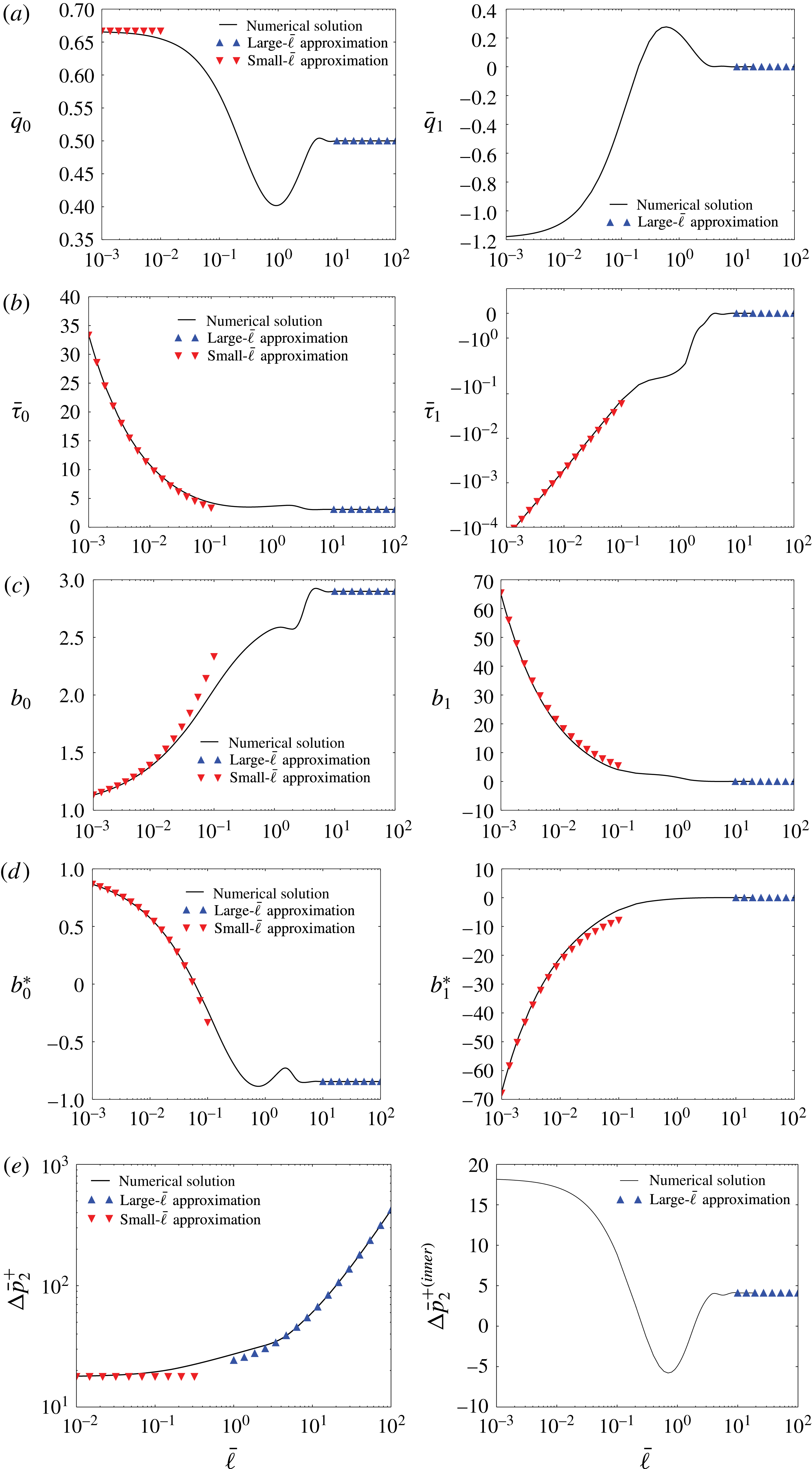
. The constants
 $\bar{q}_{0}$
,
 $\bar{\unicode[STIX]{x1D70F}}_{0}$
,
 $b_{0}$
,
 $b_{0}^{\ast }$
and
 $\unicode[STIX]{x0394}\bar{p}_{2}^{+}$
are plotted against
 $\bar{\ell }$
for
 $\bar{\unicode[STIX]{x1D6FD}}=0$
in figure 4. Results for finite values of
 $\bar{\unicode[STIX]{x1D6FD}}$
are delayed until § 7.
Gap height
 $\bar{h}$
plotted against the shifted axial coordinate
 $\bar{x}+\bar{\ell }$
for negligible bending stiffness (
 $\bar{\unicode[STIX]{x1D6FD}}=0$
). The left column is the leading-order solution
 $\bar{h}_{0}$
determined by integrating equations (5.26)–(5.30). The right column is the first correction
 $\bar{h}_{1}$
determined by integrating equations (5.48)–(5.52). The solid lines are the full numerical solutions. (a) Long, cylindrical vesicle (
 $\bar{\ell }=10$
), including the large-
 $\bar{\ell }$
approximation derived in § 6.1. (b) Intermediate length vesicle (
 $\bar{\ell }=1$
). (c) Short, spherical vesicle (
 $\bar{\ell }=0.01$
), including the small-
 $\bar{\ell }$
approximation derived in § 6.2 (cf. (6.18) and (6.26) truncated after the
 $O(1)$
term).

(a) Leakback flux
 $\bar{q}$
, (b) membrane tension
 $\bar{\unicode[STIX]{x1D70F}}$
, (c) front intercept
 $b$
, (d) rear intercept
 $b^{\ast }$
and (e) extra pressure drop
 $\unicode[STIX]{x0394}\bar{p}^{+}$
plotted against the reduced length
 $\bar{\ell }$
for negligible bending stiffness (
 $\bar{\unicode[STIX]{x1D6FD}}=0$
). The left column is the leading-order solution; the right column is the first correction.

5.3 Higher-order corrections
Corrections to the leading-order solution may be derived by expanding the narrow-gap equations to higher order in
 $\unicode[STIX]{x1D716}^{1/2}$
. In the outer region, one derives an expression similar to (5.11) for the
 $O(\unicode[STIX]{x1D716})$
shape correction:
 $$\begin{eqnarray}(1-\unicode[STIX]{x1D709}^{2})\frac{\text{d}^{2}f_{2}}{\text{d}\unicode[STIX]{x1D709}^{2}}-2\unicode[STIX]{x1D709}\frac{\text{d}f_{2}}{\text{d}\unicode[STIX]{x1D709}}+2f_{2}=2a_{2},\end{eqnarray}$$
where
 $$\begin{eqnarray}f_{2}=r_{0}r_{2},\quad a_{2}=\frac{\bar{\unicode[STIX]{x1D70F}}_{2}}{\bar{\unicode[STIX]{x1D70F}}_{0}}-\frac{\bar{p}_{2}-\hat{\bar{p}}_{2}}{\bar{p}_{0}-\hat{\bar{p}}_{0}}=\text{const}.\end{eqnarray}$$
In deriving equation (5.32), equations (5.7) and (5.15a,b
) were used to eliminate
 $r_{0}$
and
 $r_{1}$
. The boundary conditions for
 $f_{2}(\unicode[STIX]{x1D709})$
are
 $$\begin{eqnarray}\displaystyle & \displaystyle \text{as }\unicode[STIX]{x1D709}\rightarrow 0^{+}:\qquad f_{2}=-b_{0}, & \displaystyle\end{eqnarray}$$
 $$\begin{eqnarray}\displaystyle & \displaystyle \text{as }\unicode[STIX]{x1D709}\rightarrow 0^{-}:\qquad f_{2}=-b_{0}^{\ast }, & \displaystyle\end{eqnarray}$$
 $$\begin{eqnarray}\displaystyle & \displaystyle \text{at }\unicode[STIX]{x1D709}=\pm 1:\qquad f_{2}=0, & \displaystyle\end{eqnarray}$$
where a superscript ‘plus’ or ‘minus’ indicates that the boundary
 $\unicode[STIX]{x1D709}=0$
is approached in a limiting sense from positive or negative numbers, respectively. The constants
 $b_{0}$
and
 $b_{0}^{\ast }$
are known from the solution of the leading-order, inner problem. The only solution of (5.32) which satisfies (5.34)–(5.36) is
 $$\begin{eqnarray}\displaystyle & \displaystyle r_{2}=\frac{f_{2}}{\sqrt{1-\unicode[STIX]{x1D709}^{2}}}=\left\{\begin{array}{@{}ll@{}}\displaystyle -\frac{b_{0}(1-\unicode[STIX]{x1D709})}{\sqrt{1-\unicode[STIX]{x1D709}^{2}}},\quad & \text{for }\unicode[STIX]{x1D709}\in (0,1],\\ \displaystyle -\frac{b_{0}^{\ast }(1+\unicode[STIX]{x1D709})}{\sqrt{1-\unicode[STIX]{x1D709}^{2}}},\quad & \text{for }\unicode[STIX]{x1D709}\in [-1,0),\end{array}\right. & \displaystyle\end{eqnarray}$$
 $$\begin{eqnarray}\displaystyle & \displaystyle \bar{p}_{2}-\hat{\bar{p}}_{2}=\left\{\begin{array}{@{}ll@{}}-2\bar{\unicode[STIX]{x1D70F}}_{2}-2b_{0}\bar{\unicode[STIX]{x1D70F}}_{0},\quad & \text{for }\unicode[STIX]{x1D709}\in (0,1],\\ -2\bar{\unicode[STIX]{x1D70F}}_{2}-2b_{0}^{\ast }\bar{\unicode[STIX]{x1D70F}}_{0},\quad & \text{for }\unicode[STIX]{x1D709}\in [-1,0).\end{array}\right. & \displaystyle\end{eqnarray}$$
 $\bar{\unicode[STIX]{x1D70F}}_{0}$
is known from the leading-order problem,
 $\bar{\unicode[STIX]{x1D70F}}_{2}$
remains unknown. The discontinuity in the solution at
 $\unicode[STIX]{x1D709}=0$
is resolved through construction of the inner solution.
In the inner region, the
 $O(\unicode[STIX]{x1D716}^{1/2})$
correction fields are governed by the following equations and boundary conditions:
 $$\begin{eqnarray}\frac{\unicode[STIX]{x2202}\bar{u}_{1}}{\unicode[STIX]{x2202}\bar{x}}+\frac{\unicode[STIX]{x2202}\bar{v}_{1}}{\unicode[STIX]{x2202}\bar{y}}=0,\quad \frac{\unicode[STIX]{x2202}\bar{p}_{1}}{\unicode[STIX]{x2202}\bar{x}}-\frac{\unicode[STIX]{x2202}^{2}\bar{u}_{1}}{\unicode[STIX]{x2202}\bar{y}^{2}}=0,\quad \frac{\unicode[STIX]{x2202}\bar{p}_{1}}{\unicode[STIX]{x2202}\bar{y}}=0,\end{eqnarray}$$
 $$\begin{eqnarray}\frac{\unicode[STIX]{x2202}\hat{\bar{u}}_{1}}{\unicode[STIX]{x2202}\bar{x}}+\left(\frac{\unicode[STIX]{x2202}}{\unicode[STIX]{x2202}\unicode[STIX]{x1D70E}}+\frac{1}{\unicode[STIX]{x1D70E}}\right)\hat{\bar{v}}_{1}=0,\quad \frac{\unicode[STIX]{x2202}\hat{\bar{p}}_{1}}{\unicode[STIX]{x2202}\bar{x}}=0,\quad \frac{\unicode[STIX]{x2202}\hat{\bar{p}}_{1}}{\unicode[STIX]{x2202}\unicode[STIX]{x1D70E}}-\unicode[STIX]{x1D705}\frac{\unicode[STIX]{x2202}^{2}\hat{\bar{v}}_{1}}{\unicode[STIX]{x2202}\bar{x}^{2}}=0,\end{eqnarray}$$
 $$\begin{eqnarray}\displaystyle & \displaystyle \text{at }\bar{y}=0:\qquad \bar{u}_{1}=0,\quad \bar{v}_{1}=0, & \displaystyle\end{eqnarray}$$
 $$\begin{eqnarray}\displaystyle & \displaystyle \text{at }\bar{y}=\bar{h}_{0}(\bar{x}):\qquad \bar{u}_{1}=-\bar{h}_{1}\frac{\unicode[STIX]{x2202}\bar{u}_{0}}{\unicode[STIX]{x2202}\bar{y}},\quad \bar{v}_{1}=-\bar{h}_{1}\frac{\unicode[STIX]{x2202}\bar{v}_{0}}{\unicode[STIX]{x2202}\bar{y}}, & \displaystyle\end{eqnarray}$$
 $$\begin{eqnarray}\displaystyle & \displaystyle \text{at }\unicode[STIX]{x1D70E}=0:\qquad \frac{\unicode[STIX]{x2202}\hat{\bar{u}}_{1}}{\unicode[STIX]{x2202}\unicode[STIX]{x1D70E}}=0,\quad \hat{\bar{v}}_{1}=0, & \displaystyle\end{eqnarray}$$
 $$\begin{eqnarray}\displaystyle & \displaystyle \text{at }\unicode[STIX]{x1D70E}=1:\qquad \hat{\bar{u}}_{1}=0,\quad \hat{\bar{v}}_{1}=0, & \displaystyle\end{eqnarray}$$
 $$\begin{eqnarray}\displaystyle & \displaystyle \text{at }\bar{y}=\bar{h}_{0}(\bar{x}):\qquad \bar{p}_{1}-\hat{\bar{p}}_{1}=-\bar{\unicode[STIX]{x1D70F}}_{1}\left(1+\frac{\text{d}^{2}\bar{h}_{0}}{\text{d}\bar{x}^{2}}\right)-\bar{\unicode[STIX]{x1D70F}}_{0}\frac{\text{d}^{2}\bar{h}_{1}}{\text{d}\bar{x}^{2}}+\bar{\unicode[STIX]{x1D6FD}}\frac{\text{d}^{4}\bar{h}_{1}}{\text{d}\bar{x}^{4}},\quad \bar{\unicode[STIX]{x1D70F}}_{1}=\text{const.}, & \displaystyle \nonumber\\ \displaystyle & & \displaystyle\end{eqnarray}$$
 $$\begin{eqnarray}\displaystyle & \displaystyle \bar{q}_{1}=-\int _{0}^{\bar{h}_{0}(\bar{x})}\bar{u}_{1}\,\text{d}\bar{y}+\bar{h}_{1}\bar{u}_{0}|_{\bar{y}=\bar{h}_{0}(\bar{x})}=\text{const.}, & \displaystyle\end{eqnarray}$$
 $$\begin{eqnarray}\displaystyle & \displaystyle \unicode[STIX]{x0394}\bar{p}_{3}^{+}=2\left.\int _{-\infty }^{\bar{\ell }}\frac{\unicode[STIX]{x2202}\bar{u}_{1}}{\unicode[STIX]{x2202}\bar{y}}\right|_{\bar{y}=0}\,\text{d}\bar{x}^{\ast }+2\left.\int _{-\bar{\ell }}^{\infty }\frac{\unicode[STIX]{x2202}\bar{u}_{1}}{\unicode[STIX]{x2202}\bar{y}}\right|_{\bar{y}=0}\,\text{d}\bar{x}+O(1)=\text{const.} & \displaystyle\end{eqnarray}$$
The terms multiplied by
 $\bar{h}_{1}$
on the right-hand side of (5.41) and (5.45) appear as a result of transferring the boundary from
 $\bar{y}=\bar{h}(\bar{x})$
to
 $\bar{y}=\bar{h}_{0}(\bar{x})$
(Bungay & Brenner Reference Bungay and Brenner1973). Following the same procedure as in § 5.2, the first correction to the pressure gradient and extra pressure drop are derived:
 $$\begin{eqnarray}\frac{\text{d}\bar{p}_{1}}{\text{d}\bar{x}}=\frac{\text{d}(\bar{p}_{1}-\hat{\bar{p}}_{1})}{\text{d}\bar{x}}=\frac{12}{\bar{h}_{0}^{2}}\left[\frac{\bar{h}_{1}}{\bar{h}_{0}}\left(1-\frac{3\bar{q}_{0}}{\bar{h}_{0}}\right)+\frac{\bar{q}_{1}}{\bar{h}_{0}}\right],\end{eqnarray}$$
 $$\begin{eqnarray}\displaystyle \unicode[STIX]{x0394}\bar{p}_{3}^{+(inner)} & = & \displaystyle -\int _{-\infty }^{\bar{\ell }}\left[\frac{8\bar{h}_{1}}{\bar{h}_{0}^{2}}\left(1-\frac{3\bar{q}_{0}}{\bar{h}_{0}}\right)+\frac{12\bar{q}_{1}}{\bar{h}_{0}^{2}}\right]\,\text{d}\bar{x}^{\ast }\nonumber\\ \displaystyle & & \displaystyle -\,\int _{-\bar{\ell }}^{\infty }\left[\frac{8\bar{h}_{1}}{\bar{h}_{0}^{2}}\left(1-\frac{3\bar{q}_{0}}{\bar{h}_{0}}\right)+\frac{12\bar{q}_{1}}{\bar{h}_{0}^{2}}\right]\,\text{d}\bar{x},\end{eqnarray}$$
where the superscript ‘(inner)’ is ascribed to indicate that additional contributions from the outer region may contribute at this order.
It remains to calculate
 $\bar{h}_{1}(\bar{x})$
, the first correction to the gap height. Combining (5.47) with (5.44) yields an inhomogeneous differential equation for
 $\bar{h}_{1}(\bar{x})$
:
 $$\begin{eqnarray}\bar{\unicode[STIX]{x1D6FD}}\frac{\text{d}^{5}\bar{h}_{1}}{\text{d}\bar{x}^{5}}-\bar{\unicode[STIX]{x1D70F}}_{0}\frac{\text{d}^{3}\bar{h}_{1}}{\text{d}\bar{x}^{3}}-\frac{12\bar{h}_{1}}{\bar{h}_{0}^{3}}\left(1-\frac{3\bar{q}_{0}}{\bar{h}_{0}}\right)=\bar{\unicode[STIX]{x1D70F}}_{1}\frac{\text{d}^{3}\bar{h}_{0}}{\text{d}\bar{x}^{3}}+\frac{12\bar{q}_{1}}{\bar{h}_{0}^{3}}.\end{eqnarray}$$
As before, the independent variable
 $\bar{x}$
may be exchanged for
 $\bar{x}^{\ast }$
by a simple shift of origin. The boundary conditions associated with equation (5.49) are
 $$\begin{eqnarray}\displaystyle & \displaystyle \text{at }\bar{x}=-\bar{\ell },\bar{x}^{\ast }=\bar{\ell }:\quad \bar{h}_{1}=0, & \displaystyle\end{eqnarray}$$
 $$\begin{eqnarray}\displaystyle & \displaystyle \text{as }\bar{x}\rightarrow \infty :\qquad \bar{h}_{1}\rightarrow b_{1}-b_{0}\bar{x}, & \displaystyle\end{eqnarray}$$
 $$\begin{eqnarray}\displaystyle & \displaystyle \text{as }\bar{x}^{\ast }\rightarrow -\infty :\qquad \bar{h}_{1}\rightarrow b_{1}^{\ast }+b_{0}^{\ast }\bar{x}^{\ast }, & \displaystyle\end{eqnarray}$$
where
 $$\begin{eqnarray}b_{1}=-r_{3}(-1),\quad b_{1}^{\ast }=-r_{3}(-\ell +1)\end{eqnarray}$$
are constants of integration.
Equations (5.48)–(5.52) must be integrated numerically for specific values of the reduced length
 $\bar{\ell }$
and bending parameter
 $\bar{\unicode[STIX]{x1D6FD}}$
. As with all perturbation theories, the correction fields are forced by source terms that depend on the leading-order fields. Thus, any numerical solution requires accurate tabulation of
 $\bar{h}_{0}$
at discrete points in
 $\bar{x}$
. Above
 $\bar{\ell }\simeq 20$
, the system becomes numerically stiff and roundoff errors accumulate. Numerical results for
 $\bar{\unicode[STIX]{x1D6FD}}=0$
are shown in figures 3 and 4 alongside the leading-order solutions. Results for finite values of
 $\bar{\unicode[STIX]{x1D6FD}}$
are delayed until § 7.
At the next order in
 $\unicode[STIX]{x1D716}$
, the outer correction to the shape
 $r_{3}$
forces a condition on the slope of
 $\bar{h}_{2}$
in the far field. The key result from the
 $O(\unicode[STIX]{x1D716})$
inner problem is a non-constant correction to the membrane tension
 $\bar{\unicode[STIX]{x1D70F}}_{2}$
that increases monotonically from the rear tail to the front nose. The pressure jump
 $\bar{p}_{2}-\hat{\bar{p}}_{2}$
, in turn, decreases along the axial coordinate, resulting in a pressure drop of
 $O(\unicode[STIX]{x1D716})$
. Calculation of
 $r_{3}$
requires consideration of the outer flow field and is beyond the scope of the present work. Thus, further corrections are not pursued here.
6 Asymptotic solutions for
$\bar{\unicode[STIX]{x1D6FD}}=0$

6.1 Long, cylindrical vesicles
$(\bar{\ell }\gg 1)$

Asymptotic solutions of (5.26)–(5.30) and (5.48)–(5.52) may be determined when the reduced length
 $\bar{\ell }$
is either very large or very small, the former being a regular limit and the latter being a singular one. The asymptotic solution ‘for large
 $\bar{\ell }$
’ is the subject of this section. Solutions ‘for small
 $\bar{\ell }$
’ are discussed in § 6.2. In this and the subsequent section, the bending terms in the shape equations are neglected by setting
 $\bar{\unicode[STIX]{x1D6FD}}=0$
. This limit might raise concerns, since
 $\bar{\unicode[STIX]{x1D6FD}}$
is multiplying the highest derivative in (5.27) and (5.49). However, it turns out that the limit
 $\bar{\unicode[STIX]{x1D6FD}}\rightarrow 0$
is a regular one, so setting
 $\bar{\unicode[STIX]{x1D6FD}}=0$
does not preclude satisfaction of the boundary conditions. Results for finite values of
 $\bar{\unicode[STIX]{x1D6FD}}$
are discussed in § 7.
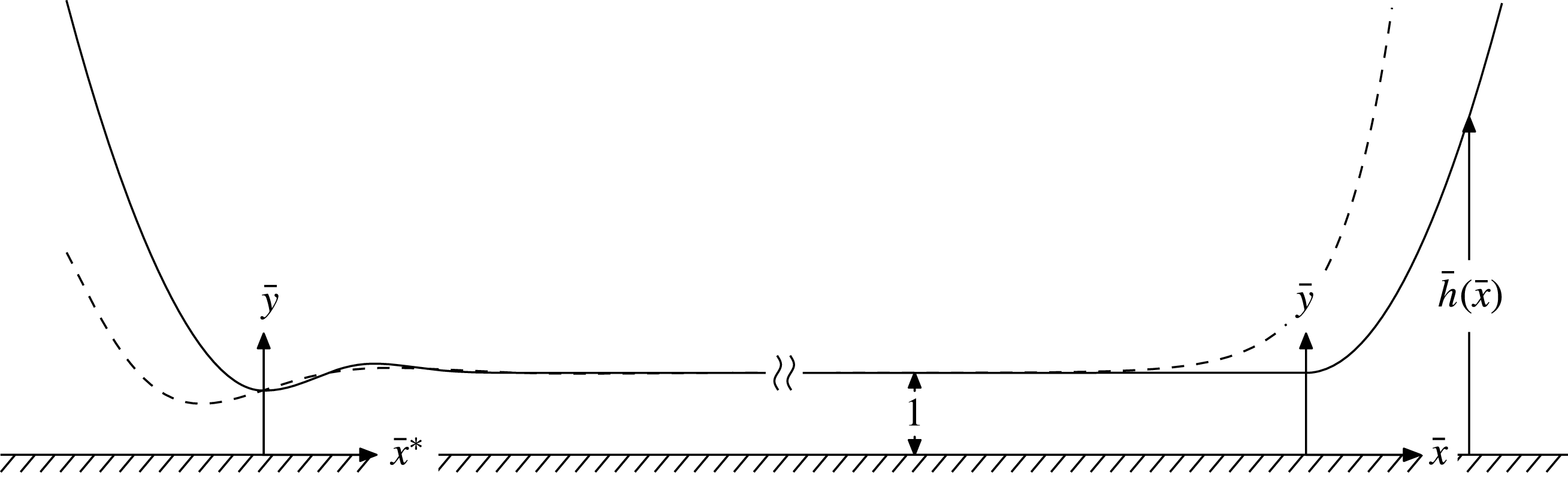
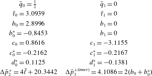
Separation of the front and rear parts of the inner region for a long, cylindrical vesicle (
 $\bar{\ell }\gg 1$
). The dashed curves are the linearized solutions near
 $\bar{h}=1$
.

As
 $\bar{\ell }\rightarrow \infty$
, the midsection of the vesicle adopts a cylindrical shape and the supporting film becomes asymptotically uniform with thickness
 $\bar{h}=1$
and flux
 $\bar{q}=1/2+O(\unicode[STIX]{x1D716})$
. A numerical solution for
 $\bar{h}_{0}$
and
 $\bar{h}_{1}$
may be derived using the procedure originally outlined by Bretherton (Reference Bretherton1961). In brief, the domain is separated into a ‘front’ and ‘rear’ part separated by a long, middle section where
 $\bar{h}=1$
, as shown in figure 5. Linearizing (5.27) (with
 $\bar{\unicode[STIX]{x1D6FD}}=0$
) about the fixed point
 $(\bar{h}_{0},\bar{q}_{0})=(1,1/2)$
yields
 $$\begin{eqnarray}\bar{\unicode[STIX]{x1D70F}}_{0}\frac{\text{d}^{3}\bar{h}_{0}}{\text{d}\bar{x}^{3}}-6(\bar{h}_{0}-1)=0.\end{eqnarray}$$
Starting from the front end of the vesicle, the dominant trajectory approaching the uniform film is an exponential profile,
 $$\begin{eqnarray}\text{as }\bar{x}\rightarrow -\infty :\qquad \bar{h}_{0}-1\rightarrow c_{0}\text{e}^{\unicode[STIX]{x1D6FE}_{0}\bar{x}},\end{eqnarray}$$
where
 $c_{0}$
is a constant of integration and
 $\unicode[STIX]{x1D6FE}_{0}=(6/\bar{\unicode[STIX]{x1D70F}}_{0})^{1/3}.$
From the rear end, the trajectory towards the uniform film oscillates in space,
 $$\begin{eqnarray}\text{as }\bar{x}^{\ast }\rightarrow \infty :\quad \bar{h}_{0}-1\rightarrow \text{e}^{-\unicode[STIX]{x1D6FE}_{0}\bar{x}^{\ast }/2}\left[c_{0}^{\ast }\cos \left(\sqrt{3}\unicode[STIX]{x1D6FE}_{0}\bar{x}^{\ast }/2\right)+d_{0}^{\ast }\sin \left(\sqrt{3}\unicode[STIX]{x1D6FE}_{0}\bar{x}^{\ast }/2\right)\right],\end{eqnarray}$$
where
 $c_{0}^{\ast }$
and
 $d_{0}^{\ast }$
are constants of integration. Equations (6.2)–(6.3) are meant to supplant (5.28) in the limit
 $(\bar{\unicode[STIX]{x1D6FD}},\bar{\ell })\rightarrow (0,\infty )$
. The front part of the shape is determined first and forced to match to (6.2), which then specifies a unique rear profile that matches to (6.3).
A similar analysis may be applied to
 $\bar{h}_{1}(\bar{x})$
. Linearizing equation (5.49) (with
 $\bar{\unicode[STIX]{x1D6FD}}=0$
) near the fixed point
 $(\bar{h}_{1},\bar{q}_{1})=(0,0)$
yields
 $$\begin{eqnarray}\bar{\unicode[STIX]{x1D70F}}_{0}\frac{\text{d}^{3}\bar{h}_{1}}{\text{d}\bar{x}^{3}}-6\bar{h}_{1}=-\frac{6\bar{\unicode[STIX]{x1D70F}}_{1}}{\bar{\unicode[STIX]{x1D70F}}_{0}}(\bar{h}_{0}-1).\end{eqnarray}$$
Equation (6.4) admits the linearized trajectories,
 $$\begin{eqnarray}\text{as }\bar{x}\rightarrow -\infty :\qquad \bar{h}_{1}\rightarrow c_{1}\text{e}^{\unicode[STIX]{x1D6FE}_{0}\bar{x}}-{\textstyle \frac{1}{3}}c_{0}(\bar{\unicode[STIX]{x1D70F}}_{1}/\bar{\unicode[STIX]{x1D70F}}_{0})\unicode[STIX]{x1D6FE}_{0}\bar{x}\text{e}^{\unicode[STIX]{x1D6FE}_{0}\bar{x}},\end{eqnarray}$$
starting from the front end and
 $$\begin{eqnarray}\text{as }\bar{x}^{\ast }\rightarrow \infty :\qquad \bar{h}_{1}\rightarrow \text{e}^{-\unicode[STIX]{x1D6FE}_{0}\bar{x}^{\ast }/2}\left[c_{1}^{\ast }\cos \left(\sqrt{3}\unicode[STIX]{x1D6FE}_{0}\bar{x}^{\ast }/2\right)+d_{1}^{\ast }\sin \left(\sqrt{3}\unicode[STIX]{x1D6FE}_{0}\bar{x}^{\ast }/2\right)\right],\end{eqnarray}$$
from the rear end. Here,
 $c_{1}$
,
 $c_{1}^{\ast }$
and
 $d_{1}^{\ast }$
are constants of integration. Equations (6.5)–(6.6) supplant (5.50) in the limit
 $(\bar{\unicode[STIX]{x1D6FD}},\bar{\ell })\rightarrow (0,\infty )$
. The second term on the right-hand side of (6.5) is the particular solution forced by the
 $\bar{\unicode[STIX]{x1D70F}}_{1}(\text{d}^{3}\bar{h}_{0}/\text{d}\bar{x}^{3})$
term in (5.49). Carrying out the numerical integration at the front end reveals that
 $\bar{\unicode[STIX]{x1D70F}}_{1}=0$
, which is why no such term appears in (6.6).
Numerical results for long, cylindrical vesicles (
 $\bar{\ell }\gg 1$
) with negligible bending stiffness (
 $\bar{\unicode[STIX]{x1D6FD}}=0$
).

Numerical solutions for
 $\bar{h}_{0}$
and
 $\bar{h}_{1}$
in the limit
 $\bar{\ell }\rightarrow \infty$
are plotted in figure 3(a) atop the numerical solutions for finite
 $\bar{\ell }$
. Numerical results for the constants
 $\bar{q}$
,
 $\bar{\unicode[STIX]{x1D70F}}$
,
 $b$
,
 $b^{\ast }$
,
 $c$
,
 $c^{\ast }$
,
 $d^{\ast }$
and
 $\unicode[STIX]{x0394}\bar{p}^{+}$
are tabulated in table 1 and plotted in figure 4 for large
 $\bar{\ell }$
. Of particular interest is the extra pressure drop,
 $$\begin{eqnarray}\unicode[STIX]{x0394}\bar{p}^{+}=2(\ell -2)\unicode[STIX]{x1D716}^{1/2}+20.3442\unicode[STIX]{x1D716}+4.1086\unicode[STIX]{x1D716}^{3/2}+O(\unicode[STIX]{x1D716}^{3/2}),\end{eqnarray}$$
where
 $(\ell /2-1)/\unicode[STIX]{x1D716}^{1/2}$
has been exchanged for
 $\bar{\ell }$
since
 $\bar{\ell }\gg 1$
. The first term on the right-hand side of (6.7) is dominant for small
 $\unicode[STIX]{x1D716}$
and arises from the dissipation in the uniform-film region. The order of this term (in physical units) is
 $O[\unicode[STIX]{x1D707}UL/(Rh^{\circ })]$
, which is in agreement with the prediction made by Halpern & Secomb (Reference Halpern and Secomb1989) and invalidates the fallacious order assignment
 $O(\unicode[STIX]{x1D707}UL^{3}/R^{4})$
given by Bruinsma (Reference Bruinsma1996). The second and third terms in (6.7) are corrections due to dissipation through the ‘transitions regions’, in which
 $\bar{h}_{0}$
deviates from unity in order to match with the outer solution. These corrections are independent of the vesicle length. Finally, the
 $O(\unicode[STIX]{x1D716}^{3/2})$
error term is meant to account for additional ‘outer contributions’, which were not computed here.
An expression similar to (6.7) was derived by Cantat (Reference Cantat2013) for the extra pressure drop across ‘no-slip bubble’ whose surface is loaded with a high concentration of insoluble surfactant. She computed a numerical value of 19.9 for the second term (when expressed in the present nomenclature). The claim here is that the discrepancy between her result and (6.7) is due to the difference in the computed values of
 $b_{0}$
and
 $b_{0}^{\ast }$
. Cantat reported
 $b_{0}=2.88$
and
 $b_{0}^{\ast }=-0.82$
, which may be compared to the values
 $b_{0}=2.8996$
and
 $b_{0}^{\ast }=-0.8453$
reported in table 1 and even Bretherton’s original calculations of
 $b_{0}=2.79$
and
 $b_{0}^{\ast }=-0.73$
. The latter values have been cited as inaccurate by Wong, Radke & Morris (Reference Wong, Radke and Morris1995), among others. The constants
 $b_{0}$
and
 $b_{0}^{\ast }$
are determined through application of the far-field conditions (5.29)–(5.30) at finite domain boundaries
 $\bar{X}$
and
 $-\bar{X}^{\ast }$
. Since
 $\bar{h}_{0}$
grows like
 $\bar{x}^{2}$
in the far field, the error in
 $\bar{h}_{0}$
incurred by truncating the domain decays like
 $1/\bar{X}$
(cf. (5.27)), which is a slow, algebraic decay. In computing the coefficients in table 1, it was found necessary to subtract off the error in successive powers of
 $1/\bar{X}$
until the computed values of
 $b_{0}$
and
 $b_{0}^{\ast }$
became independent of domain size. Thus, the reported values in table 1 were determined to an accuracy of four (or more) decimal places.
To conclude this section, it is worth quoting Bretherton’s result for the extra pressure drop across a long bubble in a tube, which when expressed in the present notation is given by
 $$\begin{eqnarray}\unicode[STIX]{x0394}\bar{p}^{+}=11.586\unicode[STIX]{x1D716}+O(\unicode[STIX]{x1D716}^{3/2}).\end{eqnarray}$$
(Equation (6.8) (in terms of outer variables) is typically expressed as
 $\unicode[STIX]{x0394}p^{+}=10.02{\mathcal{C}}^{-1/3}+O(1)$
, where
 ${\mathcal{C}}=\unicode[STIX]{x1D707}U/T$
is the capillary number and
 $T$
is the bubble surface tension. The capillary number has been eliminated using the well-known result for the clearance,
 $\unicode[STIX]{x1D716}=1.337{\mathcal{C}}^{2/3}+O({\mathcal{C}})$
.) Two important differences between (6.8) and (6.7) are worth mentioning. Firstly, it is apparent that equation (6.8) does not depend on the bubble length. This result is somewhat intuitive: since the bubble surface is shear-free, the long, cylindrical portion of the bubble does not drag fluid and so, in principle, would not contribute to the extra pressure drop. Later studies, however, have indicated a dependence on bubble length when
 $\unicode[STIX]{x1D716}$
is not vanishingly small (Schwartz, Princen & Kiss Reference Schwartz, Princen and Kiss1986). The second important difference is the numerical prefactor multiplying
 $\unicode[STIX]{x1D716}$
in (6.8), which is nearly half that of (6.7). Again, the difference can be traced to the fact that a bubble surface is a ‘shear-free surface’, whereas the vesicle membrane is treated here as a ‘no-slip surface’. The latter admits higher dissipation in the transition regions between the uniform-film and end-cap regions.
6.2 Short, spherical vesicles
$(\bar{\ell }\ll \,1)$

As
 $\bar{\ell }\rightarrow 0$
, the front nose and rear tail interact through a very short distance. The vesicle is forced into a nearly spherical shape and, consequently, the ability of the surface curvature to change in response to large lubrication pressures is dampened. In response, the membrane tension diverges to balance normal stresses on the membrane. Since the membrane is immobile, the flow field, leakback flux
 $\bar{q}$
and extra pressure drop
 $\unicode[STIX]{x0394}\bar{p}^{+}$
are adequately described by the theory for closely fitting, rigid spheres that are freely suspended in a fluid-filled tube (Hochmuth & Sutera Reference Hochmuth and Sutera1970; Bungay & Brenner Reference Bungay and Brenner1973).
The shape deformation
 $\bar{h}$
and resulting membrane tension
 $\bar{\unicode[STIX]{x1D70F}}$
for small but finite values of
 $\bar{\ell }$
are not immediately obvious. In fact, their solution in the limit of vanishing
 $\bar{\ell }$
requires a singular perturbation theory in terms of a second small parameter
 $\bar{\ell }^{1/2}\ll 1$
. In the limit
 $\bar{\ell }\rightarrow 0$
, it is convenient to shift the origin to the midplane of the vesicle,
 $$\begin{eqnarray}\bar{\unicode[STIX]{x1D709}}=\bar{x}+\bar{\ell }=\bar{x}^{\ast }-\bar{\ell },\end{eqnarray}$$
which represents the ‘outer coordinate’ for small
 $\bar{\ell }$
. The associated ‘inner coordinate’ is given by
 $$\begin{eqnarray}\tilde{\bar{\unicode[STIX]{x1D709}}}=\bar{\ell }^{1/2}\bar{\unicode[STIX]{x1D709}},\end{eqnarray}$$
where an ‘overtilde’ is used to denote a rescaling with respect to
 $\bar{\ell }^{1/2}$
. A schematic of the new coordinate system is shown in figure 6. The ‘inner region’ for small
 $\bar{\ell }$
is located in the far field (
 $\bar{\unicode[STIX]{x1D709}}\rightarrow \pm \infty$
), where
 $\bar{h}$
is very large. The width of this region is of
 $O(\bar{\ell }^{-1/2})$
. The inner solution must be matched to an outer solution near
 $\tilde{\bar{\unicode[STIX]{x1D709}}}=0$
, where
 $\bar{h}=O(1)$
.
Coordinate system for a short, spherical vesicle (
 $\bar{\ell }\ll 1$
). The ‘outer region’ is located inside the dashed box. The ‘inner region’ is located outside the dashed box within an
 $O(\bar{\ell }^{-1/2})$
boundary layer.

It is instructive at this point to derive the perturbative solution to (5.27)–(5.30) for the gap height
 $\bar{h}_{0}(\bar{\unicode[STIX]{x1D709}})$
in the limit
 $\bar{\ell }\rightarrow 0$
, setting
 $\bar{\unicode[STIX]{x1D6FD}}=0$
. Rescaling the dependent variables gives
 $$\begin{eqnarray}(\tilde{\bar{h}}_{0},\tilde{\bar{q}}_{0},\tilde{\bar{\unicode[STIX]{x1D70F}}}_{0},\tilde{b}_{0},\tilde{b}_{0}^{\ast })=(\bar{\ell }\bar{h}_{0},\bar{q}_{0},\bar{\ell }^{1/2}\bar{\unicode[STIX]{x1D70F}}_{0},b_{0},b_{0}^{\ast }).\end{eqnarray}$$
These scalings are necessary in order to satisfy all of the boundary conditions. The outer equations, which govern the unstretched gap height
 $\bar{h}_{0}(\bar{\unicode[STIX]{x1D709}})$
, are given by
 $$\begin{eqnarray}\displaystyle & \displaystyle \tilde{\bar{\unicode[STIX]{x1D70F}}}_{0}\frac{\text{d}^{3}\bar{h}_{0}}{\text{d}\bar{\unicode[STIX]{x1D709}}^{3}}=\frac{6\bar{\ell }^{1/2}}{\bar{h}_{0}^{2}}\left(1-\frac{2\bar{q}_{0}}{\bar{h}_{0}}\right), & \displaystyle\end{eqnarray}$$
 $$\begin{eqnarray}\displaystyle & \displaystyle \text{at }\bar{\unicode[STIX]{x1D709}}=0:\qquad \bar{h}_{0}=1. & \displaystyle\end{eqnarray}$$
The corresponding inner equations for the stretched gap height
 $\tilde{\bar{h}}_{0}(\tilde{\bar{\unicode[STIX]{x1D709}}})$
are
 $$\begin{eqnarray}\displaystyle & \displaystyle \tilde{\bar{\unicode[STIX]{x1D70F}}}_{0}\frac{\text{d}^{3}\tilde{\bar{h}}_{0}}{\text{d}\tilde{\bar{\unicode[STIX]{x1D709}}}^{3}}=\frac{6\bar{\ell }^{2}}{\tilde{\bar{h}}_{0}^{2}}-\frac{12\bar{\ell }^{3}\tilde{\bar{q}}_{0}}{\tilde{\bar{h}}_{0}^{3}}, & \displaystyle\end{eqnarray}$$
 $$\begin{eqnarray}\displaystyle & \displaystyle \text{as }\tilde{\bar{\unicode[STIX]{x1D709}}}\rightarrow \infty :\qquad \tilde{\bar{h}}_{0}\rightarrow {\textstyle \frac{1}{2}}\tilde{\bar{\unicode[STIX]{x1D709}}}^{2}+\bar{\ell }\tilde{b}_{0}-\bar{\ell }^{3/2}\tilde{\bar{\unicode[STIX]{x1D709}}}+{\textstyle \frac{1}{2}}\bar{\ell }^{3}, & \displaystyle\end{eqnarray}$$
 $$\begin{eqnarray}\displaystyle & \displaystyle \text{as }\tilde{\bar{\unicode[STIX]{x1D709}}}\rightarrow -\infty :\qquad \tilde{\bar{h}}_{0}\rightarrow {\textstyle \frac{1}{2}}\tilde{\bar{\unicode[STIX]{x1D709}}}^{2}+\bar{\ell }\tilde{b}_{0}^{\ast }+\bar{\ell }^{3/2}\tilde{\bar{\unicode[STIX]{x1D709}}}+{\textstyle \frac{1}{2}}\bar{\ell }^{3}. & \displaystyle\end{eqnarray}$$
The outer and inner solutions are then matched according to the matching conditions,
 $$\begin{eqnarray}\displaystyle & \displaystyle \lim _{\tilde{\bar{\unicode[STIX]{x1D709}}}\rightarrow 0^{+}}\tilde{\bar{h}}_{0}=\lim _{\bar{\unicode[STIX]{x1D709}}\rightarrow \infty }\bar{\ell }\bar{h}_{0}, & \displaystyle\end{eqnarray}$$
 $$\begin{eqnarray}\displaystyle & \displaystyle \lim _{\tilde{\bar{\unicode[STIX]{x1D709}}}\rightarrow 0^{-}}\tilde{\bar{h}}_{0}=\lim _{\bar{\unicode[STIX]{x1D709}}^{\ast }\rightarrow -\infty }\bar{\ell }\bar{h}_{0}. & \displaystyle\end{eqnarray}$$
 $\bar{\ell }^{1/2}$
, inserting the expansions into the governing equations and auxiliary conditions, and solving the resulting ordered perturbation equations in sequence. Since
 $\bar{\unicode[STIX]{x1D6FD}}$
has been set equal to zero, the composite expansion for
 $\bar{h}_{0}(\bar{\unicode[STIX]{x1D709}})$
may be derived analytically, viz.
 $$\begin{eqnarray}\displaystyle \bar{h}_{0} & = & \displaystyle 1+{\textstyle \frac{1}{2}}\bar{\unicode[STIX]{x1D709}}^{2}+\left(\frac{\sqrt{2}\bar{\ell }}{\unicode[STIX]{x03C0}}\right)^{1/2}4\arctan \left(\frac{\bar{\unicode[STIX]{x1D709}}}{\sqrt{2}}\right)+\left(\frac{\sqrt{2}\bar{\ell }}{\unicode[STIX]{x03C0}}\right)\left[-\frac{3\unicode[STIX]{x03C0}^{2}\bar{\unicode[STIX]{x1D709}}^{2}}{2}+\frac{11}{3}\left(\frac{\bar{\unicode[STIX]{x1D709}}^{2}}{1+\frac{1}{2}\bar{\unicode[STIX]{x1D709}}^{2}}\right)\right.\nonumber\\ \displaystyle & & \displaystyle +\,\left.\left(22-\frac{8}{1+\frac{1}{2}\bar{\unicode[STIX]{x1D709}}^{2}}\right)\frac{\bar{\unicode[STIX]{x1D709}}}{\sqrt{2}}\arctan \left(\frac{\bar{\unicode[STIX]{x1D709}}}{\sqrt{2}}\right)+6\bar{\unicode[STIX]{x1D709}}^{2}\arctan ^{2}\left(\frac{\bar{\unicode[STIX]{x1D709}}}{\sqrt{2}}\right)\right]\nonumber\\ \displaystyle & & \displaystyle +\,O\left[\left(\frac{\sqrt{2}\bar{\ell }}{\unicode[STIX]{x03C0}}\right)^{3/2}\right].\end{eqnarray}$$
The algebra leading to (6.18) (as well as (6.26), below) is available from the authors upon request.
A similar procedure may be applied to the solution of (5.49)–(5.52) for
 $\bar{h}_{1}(\bar{\unicode[STIX]{x1D709}})$
after setting
 $\bar{\unicode[STIX]{x1D6FD}}=0$
. The rescaled dependent variables are
 $$\begin{eqnarray}(\tilde{\bar{h}}_{1},\tilde{\bar{q}}_{1},\tilde{\bar{\unicode[STIX]{x1D70F}}}_{1},\tilde{b}_{1},\tilde{b}_{1}^{\ast })=(\bar{\ell }^{1/2}\bar{h}_{1},\bar{q}_{1},\bar{\ell }^{3/2}\bar{\unicode[STIX]{x1D70F}}_{1},\bar{\ell }^{1/2}b_{1},\bar{\ell }^{1/2}b_{1}^{\ast }).\end{eqnarray}$$
As it turns out, it is necessary to stretch
 $\bar{h}_{1}$
to
 $\tilde{\bar{h}}_{1}$
in both regions of the domain in order to formulate a consistent expansion. Using the above definitions, it is straightforward to derive the outer equations,
 $$\begin{eqnarray}\displaystyle & \displaystyle \tilde{\bar{\unicode[STIX]{x1D70F}}}_{0}\frac{\text{d}^{3}\tilde{\bar{h}}_{1}}{\text{d}\bar{\unicode[STIX]{x1D709}}^{3}}=-\frac{6\tilde{\bar{\unicode[STIX]{x1D70F}}}_{1}}{\bar{h}_{0}^{2}\tilde{\bar{\unicode[STIX]{x1D70F}}}_{0}}\left(1-\frac{2\bar{q}_{0}}{\bar{h}_{0}}\right)-\frac{12\bar{\ell }^{1/2}\tilde{\bar{h}}_{1}}{\bar{h}_{0}^{3}}\left(1-\frac{3\bar{q}_{0}}{\bar{h}_{0}}\right)-\frac{12\bar{\ell }\bar{q}_{1}}{\bar{h}_{0}^{3}}, & \displaystyle\end{eqnarray}$$
 $$\begin{eqnarray}\displaystyle & \displaystyle \text{at }\bar{\unicode[STIX]{x1D709}}=0:\qquad \tilde{\bar{h}}_{1}=0, & \displaystyle\end{eqnarray}$$
the inner equations,
 $$\begin{eqnarray}\displaystyle & \displaystyle \tilde{\bar{\unicode[STIX]{x1D70F}}}_{0}\frac{\text{d}^{3}\tilde{\bar{h}}_{1}}{\text{d}\tilde{\bar{\unicode[STIX]{x1D709}}}^{3}}=-\frac{6\bar{\ell }^{1/2}\tilde{\bar{\unicode[STIX]{x1D70F}}}_{1}}{\tilde{\bar{h}}_{0}^{2}\tilde{\bar{\unicode[STIX]{x1D70F}}}_{0}}+\frac{12\bar{\ell }^{3/2}\tilde{\bar{q}}_{0}\tilde{\bar{\unicode[STIX]{x1D70F}}}_{1}}{\tilde{\bar{h}}_{0}^{3}\tilde{\bar{\unicode[STIX]{x1D70F}}}_{0}}-\frac{12\bar{\ell }^{2}\tilde{\bar{h}}_{1}}{\tilde{\bar{h}}_{0}^{3}}-\frac{12\bar{\ell }^{5/2}\tilde{\bar{q}}_{1}}{\tilde{\bar{h}}_{0}^{3}}+\frac{36\bar{\ell }^{3}\tilde{\bar{h}}_{1}\tilde{\bar{q}}_{0}}{\tilde{\bar{h}}_{0}^{4}}, & \displaystyle\end{eqnarray}$$
 $$\begin{eqnarray}\displaystyle & \displaystyle \text{as }\tilde{\bar{\unicode[STIX]{x1D709}}}\rightarrow \infty :\qquad \tilde{\bar{h}}_{1}\rightarrow \tilde{b}_{1}-\tilde{b}_{0}\tilde{\bar{\unicode[STIX]{x1D709}}}+\bar{\ell }^{3/2}\tilde{b}_{0}, & \displaystyle\end{eqnarray}$$
 $$\begin{eqnarray}\displaystyle & \displaystyle \text{as }\tilde{\bar{\unicode[STIX]{x1D709}}}\rightarrow -\infty :\qquad \tilde{\bar{h}}_{1}\rightarrow \tilde{b}_{1}^{\ast }+\tilde{b}_{0}^{\ast }\tilde{\bar{\unicode[STIX]{x1D709}}}+\bar{\ell }^{3/2}\tilde{b}_{0}^{\ast }, & \displaystyle\end{eqnarray}$$
and the matching conditions,
 $$\begin{eqnarray}\displaystyle \lim _{\tilde{\bar{\unicode[STIX]{x1D709}}}\rightarrow 0^{+}}\tilde{\bar{h}}_{1}=\lim _{\bar{\unicode[STIX]{x1D709}}\rightarrow \infty }\tilde{\bar{h}}_{1}, & & \displaystyle\end{eqnarray}$$
 $$\begin{eqnarray}\displaystyle \lim _{\tilde{\bar{\unicode[STIX]{x1D709}}}\rightarrow 0^{-}}\tilde{\bar{h}}_{1}=\lim _{\bar{\unicode[STIX]{x1D709}}^{\ast }\rightarrow -\infty }\tilde{\bar{h}}_{1}. & & \displaystyle\end{eqnarray}$$
 $\bar{h}_{0}$
. The composite expansion for
 $\bar{h}_{1}(\bar{\unicode[STIX]{x1D709}})$
is
 $$\begin{eqnarray}\displaystyle \bar{h}_{1} & = & \displaystyle \left(\frac{\sqrt{2}}{\unicode[STIX]{x03C0}\bar{\ell }}\right)^{1/2}\left\{2\arctan \left(\frac{\bar{\unicode[STIX]{x1D709}}}{\sqrt{2}}\right)+\left(\frac{\sqrt{2}\bar{\ell }}{\unicode[STIX]{x03C0}}\right)^{1/2}\left[-\frac{3\unicode[STIX]{x03C0}^{2}\bar{\unicode[STIX]{x1D709}}^{2}}{2}+\frac{11}{3}\left(\frac{\bar{\unicode[STIX]{x1D709}}^{2}}{1+\frac{1}{2}\bar{\unicode[STIX]{x1D709}}^{2}}\right)\right.\right.\nonumber\\ \displaystyle & & \displaystyle +\,\left.\left.\left(22-\frac{8}{1+\frac{1}{2}\bar{\unicode[STIX]{x1D709}}^{2}}\right)\frac{\bar{\unicode[STIX]{x1D709}}}{\sqrt{2}}\arctan \left(\frac{\bar{\unicode[STIX]{x1D709}}}{\sqrt{2}}\right)+6\bar{\unicode[STIX]{x1D709}}^{2}\arctan ^{2}\left(\frac{\bar{\unicode[STIX]{x1D709}}}{\sqrt{2}}\right)\right]+O\left(\frac{\sqrt{2}\bar{\ell }}{\unicode[STIX]{x03C0}}\right)\!\!\right\}.\nonumber\\ \displaystyle & & \displaystyle\end{eqnarray}$$
Equations (6.18) and (6.26), truncated after the
 $O(1)$
term, are plotted in figure 3(c) atop the full numerical solutions for finite
 $\bar{\ell }$
. Analytical results for the constants
 $\bar{q}$
,
 $\bar{\unicode[STIX]{x1D70F}}$
,
 $b$
,
 $b^{\ast }$
and
 $\unicode[STIX]{x0394}\bar{p}^{+}$
are tabulated in table 2 and plotted in figure 4 for small
 $\bar{\ell }$
. The corrections
 $\bar{q}_{1}$
and
 $\unicode[STIX]{x0394}\bar{p}_{3}^{+(inner)}$
were not computed.
Analytical results for short, spherical vesicles (
 $\bar{\ell }\ll 1$
) with negligible bending stiffness (
 $\bar{\unicode[STIX]{x1D6FD}}=0$
).
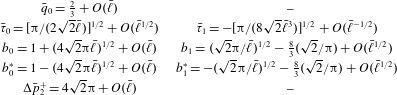
The extra pressure drop, to leading order, is given by
 $$\begin{eqnarray}\displaystyle \unicode[STIX]{x0394}\bar{p}^{+} & = & \displaystyle 4\sqrt{2}\unicode[STIX]{x03C0}\unicode[STIX]{x1D716}+O(\unicode[STIX]{x1D716}^{3/2})\nonumber\\ \displaystyle & \simeq & \displaystyle 17.7715\unicode[STIX]{x1D716}+O(\unicode[STIX]{x1D716}^{3/2}),\end{eqnarray}$$
which is simply the result for a rigid sphere that is freely suspended in a Poiseuille flow (Hochmuth & Sutera Reference Hochmuth and Sutera1970; Bungay & Brenner Reference Bungay and Brenner1973). It is noteworthy that the
 $O(\unicode[STIX]{x1D716})$
term in (6.27) is smaller than the like-ordered term in (6.7). This reduction in drag arises because the outer solution is forced to match to an inner solution with finite curvature rather than to a uniform film.
7 Effect of bending elasticity
$(\bar{\unicode[STIX]{x1D6FD}}\not =0)$

The results presented thus far have not taken into account the effect of bending elasticity. In this section, results for non-vanishing values of
 $\bar{\unicode[STIX]{x1D6FD}}$
are presented for the leading-order inner problem (5.26)–(5.30). Care must be taken when numerically integrating equation (5.27) for
 $\bar{\unicode[STIX]{x1D6FD}}\not =0$
. The general solution of the fifth-order differential equation for
 $\bar{h}_{0}(\bar{x})$
can grow exponentially in the far field, which is forbidden by the matching conditions (5.29)–(5.30). The growth rate of the dominant exponential contribution scales with either
 $\bar{\unicode[STIX]{x1D6FD}}^{1/2}$
or
 $\bar{\unicode[STIX]{x1D6FD}}^{-1/2}$
, depending on the magnitude of
 $\bar{\unicode[STIX]{x1D6FD}}$
. Consequently, the boundary-value problem becomes numerically stiff when
 $\bar{\unicode[STIX]{x1D6FD}}$
is not
 $O(1)$
. In order to circumvent this difficulty, a solution of (5.26)–(5.30) was obtained first for
 $\bar{\unicode[STIX]{x1D6FD}}=1$
, which minimizes the growth rate of the exponentials. Solutions for other values of
 $\bar{\unicode[STIX]{x1D6FD}}$
were then obtained by incrementally ‘marching’ up or down in
 $\bar{\unicode[STIX]{x1D6FD}}$
using the continuation method.
Gap height
 $\bar{h}_{0}$
plotted against the shifted axial coordinate
 $\bar{x}+\bar{\ell }$
for several values of
 $\bar{\unicode[STIX]{x1D6FD}}$
. (a) Long, cylindrical vesicle (
 $\bar{\ell }=10$
). (b) Intermediate length vesicle (
 $\bar{\ell }=1$
). (c) Short, spherical vesicle (
 $\bar{\ell }=0.01$
).

Figure 7 shows the effect of bending elasticity on
 $\bar{h}_{0}$
. Clearly, this effect is marginalized when
 $\bar{\ell }$
is small (figure 7
c). As the vesicle is forced into a spherical shape, it becomes insensitive to changes in curvature. By contrast, bending elasticity has noticeable impact on the vesicle shape when
 $\bar{\ell }$
is large (figure 7
a). The shape exhibits increasingly oscillatory behaviour in the thin-film region as
 $\bar{\unicode[STIX]{x1D6FD}}$
is increased. These oscillations may be understood by considering the linearized form of (5.27) near the fixed point
 $(\bar{h}_{0},\bar{q}_{0})=(1,1/2)$
:
 $$\begin{eqnarray}\displaystyle \bar{\unicode[STIX]{x1D6FD}}\frac{\text{d}^{5}\bar{h}_{0}}{\text{d}\bar{x}^{5}}-\bar{\unicode[STIX]{x1D70F}}_{0}\frac{\text{d}^{3}\bar{h}_{0}}{\text{d}\bar{x}^{3}}+6(\bar{h}_{0}-1)=0, & & \displaystyle\end{eqnarray}$$
which is the analogue of (6.1) for
 $\bar{\unicode[STIX]{x1D6FD}}\not =0$
. The exponential solution
 $\bar{h}_{0}=1+\text{e}^{\unicode[STIX]{x1D6FE}\bar{x}}$
admits a characteristic quintic for the eigenvalues
 $\unicode[STIX]{x1D6FE}$
:
 $$\begin{eqnarray}\bar{\unicode[STIX]{x1D6FD}}\unicode[STIX]{x1D6FE}^{5}-\bar{\unicode[STIX]{x1D70F}}_{0}\unicode[STIX]{x1D6FE}^{3}+6=0.\end{eqnarray}$$
Bruinsma (Reference Bruinsma1996) showed that the roots of (7.2) depend on the magnitude of the characteristic ratio,
 $$\begin{eqnarray}\unicode[STIX]{x1D712}=(6/\bar{\unicode[STIX]{x1D70F}}_{0})^{2/3}(\bar{\unicode[STIX]{x1D6FD}}/\bar{\unicode[STIX]{x1D70F}}_{0}),\end{eqnarray}$$
which gauges the relative importance of bending and tension in the membrane. Values of
 $\unicode[STIX]{x1D712}$
corresponding to the profiles shown in figure 7(a) are tabulated in table 3. The asymptotic solutions for the eigenvalues
 $\unicode[STIX]{x1D6FE}$
are
 $$\begin{eqnarray}\displaystyle & \displaystyle \text{as }\unicode[STIX]{x1D712}\rightarrow 0:\qquad \unicode[STIX]{x1D6FE}=(6/\bar{\unicode[STIX]{x1D70F}}_{0})^{1/3}\left\{1,\pm \sqrt{1/\unicode[STIX]{x1D712}},\text{e}^{\pm 2\unicode[STIX]{x03C0}\text{i}/3}\right\}\quad \text{(tension dominant)}, & \displaystyle\end{eqnarray}$$
 $$\begin{eqnarray}\displaystyle & \displaystyle \text{as }\unicode[STIX]{x1D712}\rightarrow \infty :\qquad \unicode[STIX]{x1D6FE}=(6/\bar{\unicode[STIX]{x1D6FD}})^{1/5}\{-1,\text{e}^{\pm \unicode[STIX]{x03C0}\text{i}/5},\text{e}^{\pm 3\unicode[STIX]{x03C0}\text{i}/5}\}\quad \text{(bending dominant)}, & \displaystyle\end{eqnarray}$$
 $\unicode[STIX]{x1D712}=\unicode[STIX]{x1D712}^{\ast }$
, where
 $$\begin{eqnarray}\unicode[STIX]{x1D712}^{\ast }=\left[\left({\textstyle \frac{3}{5}}\right)^{3/2}-\left({\textstyle \frac{3}{5}}\right)^{5/2}\right]^{2/3}\simeq 0.3257.\end{eqnarray}$$
Shape oscillations are the result of complex eigenvalues
 $\unicode[STIX]{x1D6FE}$
. When
 $\unicode[STIX]{x1D712}<\unicode[STIX]{x1D712}^{\ast }$
(the tension-dominated regime), the eigenvalues scale like
 $(6/\bar{\unicode[STIX]{x1D70F}}_{0})^{1/3}$
and are independent of
 $\bar{\unicode[STIX]{x1D6FD}}$
. Two of the real roots diverge as
 $\unicode[STIX]{x1D712}\rightarrow 0$
and hence are unphysical. The complex-valued roots are associated with the oscillatory approach to the uniform film from the rear tail (cf. (6.3)). When
 $\unicode[STIX]{x1D712}>\unicode[STIX]{x1D712}^{\ast }$
(the bending-dominated regime), the linearized shape equation gains complex eigenmodes at both ends of the uniform film. The eigenvalues in this regime scale like
 $(6/\bar{\unicode[STIX]{x1D6FD}})^{1/5}$
and are independent of
 $\bar{\unicode[STIX]{x1D70F}}_{0}$
. As
 $\unicode[STIX]{x1D712}\rightarrow \infty$
, the term multiplied by
 $\bar{\unicode[STIX]{x1D70F}}_{0}$
in (7.1) asymptotically decays, resulting in a differential balance between bending elasticity and viscous traction over a stretched increment
 $\text{d}\bar{x}=O(\bar{\unicode[STIX]{x1D6FD}}^{1/5})$
. For fixed
 $\bar{\ell }$
, this results in ‘apparent shortening’ of the thin-film region with increasing
 $\bar{\unicode[STIX]{x1D6FD}}$
, as seen in figure 7(a).
Numerical results for the membrane tension
 $\bar{\unicode[STIX]{x1D70F}}_{0}$
and characteristic ratio
 $\unicode[STIX]{x1D712}=(6/\bar{\unicode[STIX]{x1D70F}}_{0})^{2/3}(\bar{\unicode[STIX]{x1D6FD}}/\bar{\unicode[STIX]{x1D70F}}_{0})$
(cf. (7.3)) for long, cylindrical vesicles (
 $\bar{\ell }\gg 1$
) and several values of
 $\bar{\unicode[STIX]{x1D6FD}}$
. The transition between the tension- and bending-dominant eigenmodes occurs at
 $\unicode[STIX]{x1D712}^{\ast }\simeq 0.3257$
.

Leading-order solution for (a) the leakback flux
 $\bar{q}_{0}$
, (b) the membrane tension
 $\bar{\unicode[STIX]{x1D70F}}_{0}$
, (c) the front intercept
 $b_{0}$
, (d) the rear intercept
 $b_{0}^{\ast }$
and (e) the extra pressure drop
 $\unicode[STIX]{x0394}\bar{p}_{2}^{+}$
plotted against the reduced length
 $\bar{\ell }$
for several values pf
 $\bar{\unicode[STIX]{x1D6FD}}$
. Inset: curvature contribution to the extra pressure drop
 $\unicode[STIX]{x0394}\bar{p}_{2}^{+}-4\bar{\ell }$
plotted against the reduced length
 $\bar{\ell }$
.

Figure 8 extends the leading-order results of figure 4 to non-vanishing values of
 $\bar{\unicode[STIX]{x1D6FD}}$
. Although the effect of bending elasticity is non-monotonic over the range of
 $\bar{\ell }$
considered, some general trends may be deduced. The addition of bending resistance typically reduces the membrane tension
 $\bar{\unicode[STIX]{x1D70F}}_{0}$
. This is an expected effect, since bending moments can also exert an in-plane tension (Secomb Reference Secomb1988). The shape coefficients
 $b_{0}$
and
 $b_{0}^{\ast }$
also change with
 $\bar{\unicode[STIX]{x1D6FD}}$
, and in the appendix it is shown that this change has a direct consequence on the available vesicle surface area and enclosed volume. When
 $\bar{\ell }=O(1)$
, increasing
 $\bar{\unicode[STIX]{x1D6FD}}$
tends to reduce the leakback flux
 $\bar{q}_{0}$
and increase the extra pressure drop
 $\unicode[STIX]{x0394}\bar{p}_{2}^{+}$
. This trend implies that undulations in
 $\bar{h}_{0}$
result in local occlusion of flow in the thin-gap region, which hinders vesicle mobility and enhances wall resistance. As
 $\bar{\ell }$
increases, ‘stiffer vesicles’ (larger
 $\bar{\unicode[STIX]{x1D6FD}}$
) are forced into a shape that occludes most of the tube cross-section. This effect manifests in enhanced sensitivity of the constants
 $\bar{q}_{0}$
,
 $\bar{\unicode[STIX]{x1D70F}}_{0}$
,
 $b_{0}$
,
 $b_{0}^{\ast }$
and
 $\unicode[STIX]{x0394}\bar{p}_{2}^{+}$
to changes in
 $\bar{\ell }$
, as indicated by the sharp gradients between in
 $\bar{\ell }=1$
and 10 in figure 8. Since the governing equations are numerically stiff in this region of the parameter space, smaller ‘steps’ in
 $\bar{\unicode[STIX]{x1D6FD}}$
and
 $\bar{\ell }$
were required during the continuation procedure in order to ensure convergence and accuracy within the desired tolerance. When
 $\bar{\ell }$
becomes very large,
 $\bar{q}_{0}$
,
 $\bar{\unicode[STIX]{x1D70F}}_{0}$
,
 $b_{0}$
and
 $b_{0}^{\ast }$
plateau to a value that depends on
 $\bar{\unicode[STIX]{x1D6FD}}$
but not
 $\bar{\ell }$
. Changes in
 $\unicode[STIX]{x0394}\bar{p}_{2}^{+}$
are masked by a ‘cylinder contribution’ of size
 $4\bar{\ell }$
(cf. table 1). The
 $4\bar{\ell }$
contribution is subtracted out in the inset of figure 8(e) so as to isolate the ‘curvature contribution’ to
 $\unicode[STIX]{x0394}\bar{p}_{2}^{+}$
. It is seen that bending elasticity can reduce the wall drag when
 $\bar{\ell }$
is large. This result contrasts with Bruinsma’s prediction that the pressure drop across a long vesicle should be independent of membrane bending elasticity (Bruinsma Reference Bruinsma1996).
The above discussion illustrates that bending elasticity can qualitatively change the nature of the solutions to (5.27). The limit
 $\bar{\unicode[STIX]{x1D6FD}}\rightarrow \infty$
, which was briefly considered by Bruinsma (Reference Bruinsma1996), likely admits an asymptotic solution in terms of the small parameter
 $\bar{\unicode[STIX]{x1D6FD}}^{-1/5}$
. Although it is straightforward to extend the continuation method to larger values of
 $\bar{\unicode[STIX]{x1D6FD}}$
, the large-
 $\bar{\unicode[STIX]{x1D6FD}}$
asymptotic was not attempted in this work as it is not particularly relevant for most experimental conditions. This latter point may be deduced from dimensional analysis. The bending modulus of unilamellar, bilayer vesicles is approximately
 $B=10^{-12}$
erg (Evans & Needham Reference Evans and Needham1987). Taking water to be the typical working fluid (viscosity
 $\unicode[STIX]{x1D707}=1~\text{cP}$
), tube radii in the range
 $R=1{-}100~\unicode[STIX]{x03BC}\text{m}$
, and vesicle speeds in the range
 $U=1~\unicode[STIX]{x03BC}\text{m}~\text{s}^{-1}$
to
 $1~\text{cm}~\text{s}^{-1}$
, the (unstretched) bending parameter is estimated to be in the range
 $\unicode[STIX]{x1D6FD}=10^{-6}$
–
 $10^{2}$
. The stretched bending parameter
 $\bar{\unicode[STIX]{x1D6FD}}=\unicode[STIX]{x1D716}^{1/2}\unicode[STIX]{x1D6FD}$
is even smaller!
8 Elimination of
$\unicode[STIX]{x1D716}$
and
$\ell$
as parameters


The theory put forth has been parametrized in terms of four dimensionless groups (cf. (3.2)), three of which
 $(\unicode[STIX]{x1D716},\ell ,\unicode[STIX]{x1D6FD})$
depend on the local flow conditions. In order to put the results of §§ 5–7 into a more useable form, it is necessary to eliminate
 $\unicode[STIX]{x1D716}$
and
 $\ell$
in favour of ‘geometric parameters’ – i.e. those which do not depend on the local flow conditions. The geometric scales are the tube radius
 $R$
, vesicle surface area
 $A$
and enclosed volume
 $\unicode[STIX]{x1D6FA}$
. Defining the vesicle radius as
 $R_{0}=\sqrt{A/(4\unicode[STIX]{x03C0})}$
, the system geometry (irrespective of the flow field) is completely specified by two dimensionless groups (Vitkova et al.
Reference Vitkova, Mader and Podgorski2004; Trozzo et al.
Reference Trozzo, Boedec, Leonetti and Jaeger2015):
 $$\begin{eqnarray}\displaystyle & \displaystyle \unicode[STIX]{x1D710}=\frac{\unicode[STIX]{x1D6FA}}{\frac{4}{3}\unicode[STIX]{x03C0}R_{0}^{3}}\quad \text{(the reduced volume)}, & \displaystyle\end{eqnarray}$$
 $$\begin{eqnarray}\displaystyle & \displaystyle \unicode[STIX]{x1D6EC}=\frac{R_{0}}{R}\quad \text{(the radius ratio)}. & \displaystyle\end{eqnarray}$$
The reduced volume
 $\unicode[STIX]{x1D710}$
varies between 0 and 1 and gauges the ‘vesicle sphericity’ (a reduced volume of unity corresponds to a perfectly spherical vesicle). The radius ratio
 $\unicode[STIX]{x1D6EC}$
measures the size of the vesicle relative to the size of the tube, but is not normalized because the maximum value
 $\unicode[STIX]{x1D6EC}^{\ast }$
(the critical radius ratio) varies with
 $\unicode[STIX]{x1D710}$
. It is possible to determine
 $\unicode[STIX]{x1D6EC}^{\ast }$
implicitly from the equation for a spherocylinder of radius
 $R$
,
 $$\begin{eqnarray}2\unicode[STIX]{x1D710}\unicode[STIX]{x1D6EC}^{\ast 3}-3\unicode[STIX]{x1D6EC}^{\ast 2}+1=0,\end{eqnarray}$$
or explicitly via the exact solution and Taylor expansion about
 $\unicode[STIX]{x1D710}=1$
,
 $$\begin{eqnarray}\displaystyle \unicode[STIX]{x1D6EC}^{\ast } & = & \displaystyle \frac{1}{2\unicode[STIX]{x1D710}}\left[1+\left(1-2\unicode[STIX]{x1D710}^{2}+2\unicode[STIX]{x1D710}\sqrt{\unicode[STIX]{x1D710}^{2}-1}\right)^{-1/3}+\left(1-2\unicode[STIX]{x1D710}^{2}+2\unicode[STIX]{x1D710}\sqrt{\unicode[STIX]{x1D710}^{2}-1}\right)^{1/3}\right]\end{eqnarray}$$
 $$\begin{eqnarray}\displaystyle & = & \displaystyle 1+\sqrt{\frac{2}{3}(1-\unicode[STIX]{x1D710})}+\frac{7}{9}(1-\unicode[STIX]{x1D710})+\frac{101}{54}\sqrt{\frac{1}{6}(1-\unicode[STIX]{x1D710})}^{3}+\frac{184}{243}(1-\unicode[STIX]{x1D710})^{2}+O\left(\sqrt{1-\unicode[STIX]{x1D710}}^{5}\right).\nonumber\\ \displaystyle & & \displaystyle\end{eqnarray}$$
 $\unicode[STIX]{x1D6EC}^{\ast }$
against
 $\unicode[STIX]{x1D710}$
is shown in figure 9. The ratio
 $\unicode[STIX]{x1D6EC}/\unicode[STIX]{x1D6EC}^{\ast }$
is properly normalized so that a value of unity denotes the maximum vesicle size for a given tube radius. If
 $\unicode[STIX]{x1D6EC}>\unicode[STIX]{x1D6EC}^{\ast }$
, the vesicle cannot pass through the tube without rupturing. Experiments with swollen red blood cells (reduced volume
 $\unicode[STIX]{x1D710}\simeq 0.9$
) indicate that lysis occurs above
 $\unicode[STIX]{x1D6EC}^{\ast }\simeq 1.5$
(Savin, Bandi & Mahadevan Reference Savin, Bandi and Mahadevan2016), which is in excellent agreement with the theoretical prediction of
 $1.4$
from (8.4a
).
Critical radius ratio
 $\unicode[STIX]{x1D6EC}^{\ast }$
plotted against the reduced volume
 $\unicode[STIX]{x1D710}$
. The exact solution and Taylor series near
 $\unicode[STIX]{x1D710}=1$
are given by (8.4a
) and (8.4b
), respectively. Membrane rupture occurs for
 $\unicode[STIX]{x1D6EC}>\unicode[STIX]{x1D6EC}^{\ast }$
, as indicated by the shaded region.

The clearance parameter
 $\unicode[STIX]{x1D716}$
and reduced length
 $\ell$
, which were the appropriate parameters for constructing the narrow-gap perturbation theory, may now be eliminated in favour of the geometric parameters
 $\unicode[STIX]{x1D6EC}$
and
 $\unicode[STIX]{x1D6EC}^{\ast }$
. The following expansions are derived in the appendix:
 $$\begin{eqnarray}\displaystyle & \displaystyle \unicode[STIX]{x1D716}=1-\unicode[STIX]{x1D706}+O[(1-\unicode[STIX]{x1D706})^{2}], & \displaystyle\end{eqnarray}$$
 $$\begin{eqnarray}\displaystyle & \displaystyle \ell /2={\unicode[STIX]{x1D6EC}^{\ast }}^{2}-[1+{\unicode[STIX]{x1D6EC}^{\ast }}^{2}-{\textstyle \frac{1}{2}}(b_{0}+b_{0}^{\ast })](1-\unicode[STIX]{x1D706})+O[(1-\unicode[STIX]{x1D706})^{2}], & \displaystyle\end{eqnarray}$$
where
 $\unicode[STIX]{x1D706}=\unicode[STIX]{x1D6EC}/\unicode[STIX]{x1D6EC}^{\ast }$
is the reduced radius ratio. The coefficients
 $b_{0}$
and
 $b_{0}^{\ast }$
depend the stretched parameters
 $\bar{\ell }$
and
 $\bar{\unicode[STIX]{x1D6FD}}$
(shown in figure 8
c,d) and hence vary with both geometry and flow conditions. The error terms neglected in (8.5)–(8.6) can also depend on the flow conditions. By using equations (8.5)–(8.6), it is possible to eliminate
 $\unicode[STIX]{x1D716}$
and
 $\ell$
from the theory entirely and parametrize the results of the previous sections in terms of the reduced volume
 $\unicode[STIX]{x1D710}$
, radius ratio
 $\unicode[STIX]{x1D6EC}$
and (unstretched) bending parameter
 $\unicode[STIX]{x1D6FD}$
. The utility of this alternative parametrization is that
 $\unicode[STIX]{x1D710}$
and
 $\unicode[STIX]{x1D6EC}$
are purely geometric quantities, with all of the dynamical information contained in
 $\unicode[STIX]{x1D6FD}$
. The limit
 $\unicode[STIX]{x1D716}\rightarrow 0$
is directly mapped to
 $\unicode[STIX]{x1D6EC}\rightarrow \unicode[STIX]{x1D6EC}^{\ast }$
(or
 $\unicode[STIX]{x1D706}\rightarrow 1$
).
Vesicle shapes for fixed
 $\unicode[STIX]{x1D710}$
,
 $\unicode[STIX]{x1D706}$
and
 $\unicode[STIX]{x1D6FD}$
are shown in figure 10. The shapes were generated by additive composition of the outer and inner expansions for
 $r(x)=1-h(x)$
(van Dyke Reference van Dyke1964). The shape change between
 $\unicode[STIX]{x1D6FD}=0$
and
 $10$
is nearly indiscernible – except when
 $\unicode[STIX]{x1D710}$
and
 $\unicode[STIX]{x1D706}$
are small – because confinement suppresses bending elasticity. As
 $\unicode[STIX]{x1D706}$
is increased (for fixed
 $\unicode[STIX]{x1D710}$
), the narrow gap widens and the vesicle elongates. Vesicles of lower reduced volume
 $\unicode[STIX]{x1D710}$
(for fixed
 $\unicode[STIX]{x1D706}$
) tend to be longer; setting
 $\unicode[STIX]{x1D706}=1$
yields an explicit expression for the reduced length
 $\ell$
in terms of
 $\unicode[STIX]{x1D710}$
:
 $$\begin{eqnarray}\displaystyle \lim _{\unicode[STIX]{x1D706}\rightarrow 1}\ell /2=1+2\sqrt{{\textstyle \frac{2}{3}}(1-\unicode[STIX]{x1D710})}+{\textstyle \frac{20}{9}}(1-\unicode[STIX]{x1D710})+O\left(\sqrt{1-\unicode[STIX]{x1D710}}^{3}\right), & & \displaystyle\end{eqnarray}$$
which shows that decreasing
 $\unicode[STIX]{x1D710}$
tends to increase
 $\ell$
if the vesicle is ‘sphere-like’ (
 $\unicode[STIX]{x1D710}$
close to unity).
Vesicle shapes for several values of the reduced volume
 $\unicode[STIX]{x1D710}$
and reduced radius ratio
 $\unicode[STIX]{x1D706}$
: (a)
 $\unicode[STIX]{x1D710}=0.99$
, (b)
 $\unicode[STIX]{x1D710}=0.95$
, (c)
 $\unicode[STIX]{x1D710}=0.90$
, (d)
 $\unicode[STIX]{x1D710}=0.85$
, (e)
 $\unicode[STIX]{x1D710}=0.80$
, (f)
 $\unicode[STIX]{x1D710}=0.75$
, (g)
 $\unicode[STIX]{x1D710}=0.70$
, (h)
 $\unicode[STIX]{x1D710}=0.65$
and (e)
 $\unicode[STIX]{x1D710}=0.60$
. Left column:
 $\unicode[STIX]{x1D6FD}=0$
. Right column:
 $\unicode[STIX]{x1D6FD}=10$
.

Velocity ratio
 $U/V$
and dimensionless extra pressure drop
 $\unicode[STIX]{x0394}p^{+}U/V$
for different values of the reduced volume
 $\unicode[STIX]{x1D710}$
, reduced radius ratio
 $\unicode[STIX]{x1D706}$
(or radius ratio
 $\unicode[STIX]{x1D6EC}$
, also shown) and bending parameter
 $\unicode[STIX]{x1D6FD}$
. The clearance parameter is in the range
 $0<\unicode[STIX]{x1D716}<0.3$
.

The most important hydrodynamical quantities of interest are the speed ratio
 $U/V=(1-2q)^{-1}$
and dimensionless extra pressure drop
 $\unicode[STIX]{x0394}p^{+}U/V$
(here scaled with respect to the mean flow speed
 $V$
instead of the vesicle speed
 $U$
). These quantities were calculated from composite expansions and the numerical results are tabulated in table 4 for fixed
 $\unicode[STIX]{x1D710}$
,
 $\unicode[STIX]{x1D706}$
and
 $\unicode[STIX]{x1D6FD}$
. The vesicle mobility (measured by the speed ratio
 $U/V$
) is relatively unchanged across reduced volumes
 $\unicode[STIX]{x1D710}$
so long as the reduced radius ratio
 $\unicode[STIX]{x1D706}$
is kept constant. This is because the effective cross-sectional area occluded by the vesicle is independent of the vesicle length. On the other hand, the wall resistance (measured by the dimensionless extra pressure drop
 $\unicode[STIX]{x0394}p^{+}U/V$
) is highly sensitive to
 $\unicode[STIX]{x1D710}$
because the drag scales linearly with the vesicle length (cf. (6.7)). As shown in table 4, the value of
 $\unicode[STIX]{x1D706}$
for which
 $\unicode[STIX]{x0394}p^{+}U/V\approx 80$
decreases as
 $\unicode[STIX]{x1D710}$
is decreased.
The asymptotic behaviour of
 $U/V$
and
 $\unicode[STIX]{x0394}p^{+}U/V$
as
 $\unicode[STIX]{x1D706}\rightarrow 1$
(maximum confinement) depends on the vesicle shape. Two limiting cases for
 $\unicode[STIX]{x1D6FD}=0$
were considered in § 6, which correspond to either long, cylindrical vesicles (
 $\unicode[STIX]{x1D710}<1$
,
 $\unicode[STIX]{x1D6EC}^{\ast }>1$
) or short, spherical vesicles (
 $\unicode[STIX]{x1D710}\simeq 1$
,
 $\unicode[STIX]{x1D6EC}^{\ast }\simeq 1$
). After using equations (8.5)–(8.6) to eliminate
 $\unicode[STIX]{x1D716}$
and
 $\ell$
, the asymptotes may be written in terms of the geometric parameters
 $\unicode[STIX]{x1D706}$
and
 $\unicode[STIX]{x1D6EC}^{\ast }$
. These results summarized in table 5. Savin et al. (Reference Savin, Bandi and Mahadevan2016) showed that separate results for cylinders and spheres may be unified by interpolating over the reduced length
 $\ell =2{\unicode[STIX]{x1D6EC}^{\ast }}^{2}+O(1-\unicode[STIX]{x1D706})$
. In this spirit, the following approximate expressions nicely interpolate the results presented in table 5 for all reduced volumes:
 $$\begin{eqnarray}\displaystyle & \displaystyle \lim _{\unicode[STIX]{x1D706}\rightarrow 1}\frac{U}{V}\simeq 1+\frac{4}{3}\left(\frac{3{\unicode[STIX]{x1D6EC}^{\ast }}^{2}-2}{4{\unicode[STIX]{x1D6EC}^{\ast }}^{2}-3}\right)(1-\unicode[STIX]{x1D706}), & \displaystyle\end{eqnarray}$$
 $$\begin{eqnarray}\displaystyle & \displaystyle \lim _{\unicode[STIX]{x1D706}\rightarrow 1}\frac{\unicode[STIX]{x0394}p^{+}U}{V}\simeq \frac{4({\unicode[STIX]{x1D6EC}^{\ast }}^{2}-1)}{1-\unicode[STIX]{x1D706}}\left[1+\left(\frac{\sqrt{2}\unicode[STIX]{x03C0}}{(4{\unicode[STIX]{x1D6EC}^{\ast }}^{2}-3)({\unicode[STIX]{x1D6EC}^{\ast }}^{2}-1)}\right)(1-\unicode[STIX]{x1D706})^{1/2}\right]. & \displaystyle\end{eqnarray}$$
Equations (8.8)–(8.9) are the most practical results of this paper. Since bending elasticity has a negligible effect for most reasonable values of
 $\unicode[STIX]{x1D6FD}$
, it is expected that these expressions will be insensitive to the flow conditions. Thus, the predictions for
 $U/V$
and
 $\unicode[STIX]{x0394}p^{+}U/V$
under high confinement are set entirely by the geometry of the system.


9 Discussion of results
9.1 Review of assumptions
The narrow-gap theory presented in this paper was developed after making several assumptions other than the obvious restriction
 $\unicode[STIX]{x1D716}\ll 1$
. These include
-
(i) inertialessness,
-
(ii) weightlessness,
-
(iii) axisymmetry,
-
(iv) steadiness.
It is instructive at this point to justify these assumptions. In doing so, it will become necessary to introduce some new dimensional parameters that were previously omitted. In the forthcoming section, tube radii in the range
 $R=1{-}100~\unicode[STIX]{x03BC}\text{m}$
and vesicle speeds in the range
 $U=1~\unicode[STIX]{x03BC}\text{m}~\text{s}^{-1}$
to
 $1~\text{cm}~\text{s}^{-1}$
will be assumed, as these are typical working parameters in microfluidic experiments (Squires & Quake Reference Squires and Quake2005).
(i) Neglect of inertial forces in the equations of motion (2.4) is justified so long as the Reynolds number
 ${\mathcal{R}}=\unicode[STIX]{x1D70C}RU/\unicode[STIX]{x1D707}$
is sufficiently small, where
 $\unicode[STIX]{x1D70C}$
is the exterior fluid density (the interior fluid density being
 $\hat{\unicode[STIX]{x1D70C}}$
). In the context of the narrow-gap assumption, one requires
 $$\begin{eqnarray}\bar{{\mathcal{R}}}=\unicode[STIX]{x1D716}{\mathcal{R}}\ll 1\end{eqnarray}$$
for inertial forces to be neglected in the exterior fluid. A similar condition may be written for the interior fluid. Using water as the typical working fluid (viscosity
 $\unicode[STIX]{x1D707}=1~\text{cP}$
and density
 $\unicode[STIX]{x1D70C}=1~\text{g}~\text{cm}^{-3}$
), the Reynolds number is estimated to be in the range
 ${\mathcal{R}}=10^{-6}-1$
. Thus, equation (9.1) is always satisfied so long as
 $\unicode[STIX]{x1D716}\ll 1$
.
(ii) The fluid pressures
 $p$
and
 $\hat{p}$
were made ‘dynamic’ by subtracting the hydrostatic contribution
 $\unicode[STIX]{x1D70C}\boldsymbol{g}\boldsymbol{\cdot }\boldsymbol{x}$
and
 $\hat{\unicode[STIX]{x1D70C}}\boldsymbol{g}\boldsymbol{\cdot }\boldsymbol{x}$
, respectively, where
 $\boldsymbol{g}$
is the acceleration due to gravity. Defining the ‘gravity number’ as
 ${\mathcal{G}}=|\unicode[STIX]{x1D70C}-\hat{\unicode[STIX]{x1D70C}}|gR^{2}/(\unicode[STIX]{x1D707}U)$
(Leal Reference Leal2007) with
 $g\equiv |\boldsymbol{g}|=9.8~\text{m}~\text{s}^{-2}$
, gravitational terms may be neglected in the normal stress condition (2.9a
) so long as
 $$\begin{eqnarray}\bar{{\mathcal{G}}}=\unicode[STIX]{x1D716}^{3/2}{\mathcal{G}}\ll 1.\end{eqnarray}$$
Equation (9.2) is typically satisfied if the exterior and interior fluids have nearly equal density (a neutrally buoyant vesicle). The factor of
 $\unicode[STIX]{x1D716}^{3/2}$
in (9.2) diminishes the effect of non-neutral buoyancy. Assuming the largest density difference to be
 $|\unicode[STIX]{x1D70C}-\hat{\unicode[STIX]{x1D70C}}|=0.1~\text{g}~\text{cm}^{-3}$
, the gravity number is estimated to be in the range
 ${\mathcal{G}}=10^{-4}{-}10^{4}$
, with the largest gravity numbers corresponding to small velocities and large tube radii. It is possible for gravitational effects to play a role under these latter conditions.
(iii) Only axisymmetric vesicle shapes are reported in this work, raising the question as to whether non-axisymmetric solutions exist. Since the azimuthal coordinate
 $\unicode[STIX]{x1D719}$
is not stretched in the small-
 $\unicode[STIX]{x1D716}$
expansion,
 $$\begin{eqnarray}\frac{|\unicode[STIX]{x2202}^{2}h/\unicode[STIX]{x2202}\unicode[STIX]{x1D719}^{2}|}{|\unicode[STIX]{x2202}^{2}h/\unicode[STIX]{x2202}x^{2}|}=\unicode[STIX]{x1D716}\left(\frac{|\unicode[STIX]{x2202}^{2}\bar{h}/\unicode[STIX]{x2202}\unicode[STIX]{x1D719}^{2}|}{|\unicode[STIX]{x2202}^{2}\bar{h}/\unicode[STIX]{x2202}\bar{x}^{2}|}\right)=O(\unicode[STIX]{x1D716}),\end{eqnarray}$$
which implies that the change in the azimuthal curvature due to variations of
 $h$
along
 $\unicode[STIX]{x1D719}$
is small relative to the meridional curvature. Thus, non-axisymmetric solutions do not enter into the leading-order theory if
 $\unicode[STIX]{x1D716}\ll 1$
.
(iv) The steady-state form of the kinematic condition,
 $\text{d}q/\text{d}x=0$
, was used in the development of the narrow-gap theory. The unsteady form is
 $$\begin{eqnarray}\frac{\unicode[STIX]{x2202}h}{\unicode[STIX]{x2202}t}+\frac{\unicode[STIX]{x2202}q}{\unicode[STIX]{x2202}x}=0,\end{eqnarray}$$
where
 $t$
is the time variable (scaled by
 $R/U$
). Rescaling
 $\bar{t}=t/\unicode[STIX]{x1D716}$
and eliminating
 $q$
from the expression, one obtains at leading order,
 $$\begin{eqnarray}\frac{\unicode[STIX]{x2202}\bar{h}_{0}}{\unicode[STIX]{x2202}\bar{t}}-\frac{\unicode[STIX]{x2202}}{\unicode[STIX]{x2202}\bar{x}}\left[\frac{\bar{h}_{0}}{2}+\frac{\bar{h}_{0}^{3}}{12}\left(\bar{\unicode[STIX]{x1D6FD}}\frac{\unicode[STIX]{x2202}^{5}\bar{h}_{0}}{\unicode[STIX]{x2202}\bar{x}^{5}}-\bar{\unicode[STIX]{x1D70F}}_{0}\frac{\unicode[STIX]{x2202}^{3}\bar{h}_{0}}{\unicode[STIX]{x2202}\bar{x}^{3}}\right)\right]=0.\end{eqnarray}$$
Equation (9.5) is the unsteady analogue of (5.27). The linear stability of
 $\bar{h}_{0}(\bar{x},\bar{t})$
near the fixed point
 $\bar{h}_{0}=1$
is analysed by introducing a Fourier perturbation
 $\bar{h}_{0}(\bar{x},\bar{t})=1+\unicode[STIX]{x1D6FF}\text{e}^{\unicode[STIX]{x1D714}\bar{t}+\text{i}k\bar{x}}$
, where
 $\unicode[STIX]{x1D6FF}$
is the amplitude,
 $\unicode[STIX]{x1D714}$
is the frequency and
 $k$
is the wavenumber. After neglecting
 $O(\unicode[STIX]{x1D6FF}^{2})$
terms, the dispersion relationship between
 $\unicode[STIX]{x1D714}$
and
 $k$
is found to be
 $$\begin{eqnarray}\unicode[STIX]{x1D714}=-{\textstyle \frac{1}{12}}(\bar{\unicode[STIX]{x1D6FD}}k^{6}+\bar{\unicode[STIX]{x1D70F}}_{0}k^{4})+{\textstyle \frac{1}{2}}\text{i}k.\end{eqnarray}$$
Equation (9.6) indicates that the Fourier perturbations are travelling waves with phase speed
 $k/2$
. The waves decay in time so long as
 $\bar{\unicode[STIX]{x1D70F}}_{0}+\bar{\unicode[STIX]{x1D6FD}}k^{2}>0$
. Thus, the membrane is stable to small-amplitude perturbations when under tension (
 $\bar{\unicode[STIX]{x1D70F}}_{0}>0$
). It is not possible, under the auspices of the theory, for the vesicle to be put under compression (
 $\bar{\unicode[STIX]{x1D70F}}_{0}<0$
), as can occur when the vesicle is freely suspended in a quiescent fluid. Since it was previously stipulated that
 $\bar{\unicode[STIX]{x1D6FD}}=O(\unicode[STIX]{x1D716}^{-1/2})$
, the viscous stress term in (5.27) remains dominant for any choice of the parameters. As
 $\bar{\unicode[STIX]{x1D6FD}}$
increases, the membrane tension
 $\bar{\unicode[STIX]{x1D70F}}_{0}$
decreases in magnitude (but remains positively valued), resulting in a balance between curvature elasticity and viscous stress in (5.27).
The crucial criteria for shape stability were
 $\unicode[STIX]{x1D716}\ll 1$
and
 $\bar{\unicode[STIX]{x1D6FD}}=O(\unicode[STIX]{x1D716}^{-1/2})$
. For larger values of
 $\unicode[STIX]{x1D716}$
, it is possible for the membrane tension to balance (even locally) the curvature-elastic term in (5.27). When this balance occurs, the membrane tension can become negatively valued and locally flat sections of membrane become linearly unstable to large-wavenumber perturbations. Schwartz et al. (Reference Schwartz, Princen and Kiss1986) also showed that variations in the azimuthal curvature can become non-negligible and destabilizing when
 $\unicode[STIX]{x1D716}$
is not small.
9.2 Comparison to direct numerical simulations
Trozzo et al. (Reference Trozzo, Boedec, Leonetti and Jaeger2015) performed axisymmetric boundary element simulations of vesicles flowing in capillary tubes. A comparison of the present theory to their results for the radius of curvature
 $r=1-h$
and membrane traction
 $\boldsymbol{f}=(\unicode[STIX]{x1D64E}-\hat{\unicode[STIX]{x1D64E}})\boldsymbol{\cdot }\boldsymbol{n}$
is shown in figure 11 for two sets of the parameters
 $\unicode[STIX]{x1D710}$
,
 $\unicode[STIX]{x1D6EC}$
and
 $\unicode[STIX]{x1D6FD}$
(also reported are the associated parameters
 $\unicode[STIX]{x1D716}$
,
 $\bar{\ell }$
and
 $\bar{\unicode[STIX]{x1D6FD}}$
used in the perturbation theory).
Comparison of the present theoretical predictions for vesicle shape
 $r$
and traction components
 $f_{x}$
and
 $f_{\unicode[STIX]{x1D70E}}$
to the boundary element simulations of Trozzo et al. (Reference Trozzo, Boedec, Leonetti and Jaeger2015) (viscosity ratio
 $\unicode[STIX]{x1D705}=1$
). Results are shown for (a)
 $\unicode[STIX]{x1D710}=0.84$
,
 $\unicode[STIX]{x1D6EC}=1.2$
,
 $\unicode[STIX]{x1D6FD}=0.01$
(
 $\unicode[STIX]{x1D716}=0.22$
,
 $\bar{\ell }=1.6$
,
 $\bar{\unicode[STIX]{x1D6FD}}=0.006$
) and (b)
 $\unicode[STIX]{x1D710}=0.61$
,
 $\unicode[STIX]{x1D6EC}=2.1$
,
 $\unicode[STIX]{x1D6FD}=0.03$
(
 $\unicode[STIX]{x1D716}=0.057$
,
 $\bar{\ell }=16$
,
 $\bar{\unicode[STIX]{x1D6FD}}=0.008$
).

The agreement between the theory and the simulations improves with decreasing
 $\unicode[STIX]{x1D716}$
, as expected. The theoretical prediction for the radial component of the membrane traction
 $f_{\unicode[STIX]{x1D70E}}$
exhibits the largest discrepancy with the simulation result. Whereas the simulation reports a linearly increasing profile over the majority of the thin-film region, the perturbative result is mostly flat. This discrepancy is due to the neglect of higher-order perturbative corrections that scale linearly with
 $\bar{\ell }$
. The radial traction
 $f_{\unicode[STIX]{x1D70E}}$
is approximately given by the radial projection of the pressure jump vector
 $-(p-\hat{p})|_{\unicode[STIX]{x1D70E}=r(x)}\boldsymbol{n}$
, which is expanded up to first order in
 $\unicode[STIX]{x1D716}^{1/2}$
in this work:
 $$\begin{eqnarray}(p-\hat{p})|_{\unicode[STIX]{x1D70E}=r(x)}=\unicode[STIX]{x1D716}^{-3/2}[\bar{p}_{0}-\hat{\bar{p}}_{0}+\unicode[STIX]{x1D716}^{1/2}(\bar{p}_{1}-\hat{\bar{p}}_{1})+O(\unicode[STIX]{x1D716},\unicode[STIX]{x1D716}\bar{\ell })].\end{eqnarray}$$
Since
 $\unicode[STIX]{x0394}\bar{p}_{2}^{+}\sim 4\bar{\ell }$
, according to (6.7), the coefficient
 $\bar{p}_{2}-\hat{\bar{p}}_{2}$
of the next term in the asymptotic series must be a function that decreases by an amount
 $4\bar{\ell }$
through the thin-film region. This inner correction forces an outer correction to the rear pressure that is
 $O(\unicode[STIX]{x1D716}\bar{\ell })$
.
By contrast, both the vesicle radius
 $r$
and the axial component of the membrane traction
 $f_{x}$
are well approximated by the perturbation theory within the front nose and thin-film regions. Significant errors in these functions are only observed at the rear tail – again, due to the neglect of
 $O(\unicode[STIX]{x1D716}\bar{\ell })$
terms in the perturbative solution. In the thin-film region, the dominant contribution to
 $f_{x}$
is the membrane shear stress
 $(\unicode[STIX]{x2202}u/\unicode[STIX]{x2202}\unicode[STIX]{x1D70E})|_{\unicode[STIX]{x1D70E}=r(x)}$
:
 $$\begin{eqnarray}\left.\frac{\unicode[STIX]{x2202}u}{\unicode[STIX]{x2202}\unicode[STIX]{x1D70E}}\right|_{\unicode[STIX]{x1D70E}=r(x)}=-\unicode[STIX]{x1D716}^{-1}\left(\left.\frac{\unicode[STIX]{x2202}\bar{u}_{0}}{\unicode[STIX]{x2202}\bar{y}}\right|_{\bar{y}=\bar{h}_{0}(\bar{x})}+\unicode[STIX]{x1D716}^{1/2}\left.\frac{\unicode[STIX]{x2202}\bar{u}_{1}}{\unicode[STIX]{x2202}\bar{y}}\right|_{\bar{y}=\bar{h}_{0}(\bar{x})}+O(\unicode[STIX]{x1D716},\unicode[STIX]{x1D716}\bar{\ell })\right).\end{eqnarray}$$
The agreement with the perturbation theory is therefore expected, since the small-
 $\unicode[STIX]{x1D716}$
assumption resolves parallel flow (and, therefore, shear stresses) within the narrow gap. The fact that shear stresses are more well resolved by the perturbation theory than normal stresses is important for calculating the dimensionless extra pressure drop
 $\unicode[STIX]{x0394}p^{+}U/V$
, which is given by the resultant of shear stresses on the tube wall.
9.3 Comparison to experiments and previous theories
In figure 12, predictions for the speed ratio
 $U/V$
and dimensionless extra pressure drop
 $\unicode[STIX]{x0394}p^{+}U/V$
are compared to available experimental measurements for vesicles and red blood cells in capillary flow. Both the composite expansions (solid lines) as well as the asymptotic interpolants (8.8)–(8.9) (dashed lines) are plotted.
(a) Velocity ratio
 $U/V$
and (b) dimensionless extra pressure drop
 $\unicode[STIX]{x0394}p^{+}U/V$
plotted against the radius ratio
 $\unicode[STIX]{x1D6EC}$
for
 $\unicode[STIX]{x1D6FD}=0$
and several reduced volumes
 $\unicode[STIX]{x1D710}$
. Also shown are the experimental measurements of Vitkova et al. (Reference Vitkova, Mader and Podgorski2004), Ahmmed et al. (Reference Ahmmed, Suteria, Garbin and Vanapalli2017) (for vesicles), Albrecht et al. (Reference Albrecht, Gaehtgens, Pries and Heuser1979) and Pries, Neuhaus & Gaehtgens (Reference Pries, Neuhaus and Gaehtgens1992) (for red blood cells) as well as previous theories due to Secomb et al. (Reference Secomb, Skalak, Oozkaya and Gross1986) and Halpern & Secomb (Reference Halpern and Secomb1989) (for red blood cells).

Measurements of
 $U/V$
for vesicles in circular capillaries (
 $\unicode[STIX]{x1D710}=0.924{-}0.999$
) and square channels (
 $\unicode[STIX]{x1D710}=0.80{-}1$
) were collected by Vitkova et al. (Reference Vitkova, Mader and Podgorski2004) and Ahmmed et al. (Reference Ahmmed, Suteria, Garbin and Vanapalli2017), respectively. Unfortunately, experimental measurements of
 $\unicode[STIX]{x0394}p^{+}U/V$
for vesicles in channel flow are currently unavailable. The experimental data compiled from Albrecht et al. (Reference Albrecht, Gaehtgens, Pries and Heuser1979) and Pries et al. (Reference Pries, Neuhaus and Gaehtgens1992) are for suspensions of red blood cells flowing in capillary tubes at various volume concentrations (or ‘haematocrits’). Other reported measurements (e.g. those of Tomaiuolo et al. (Reference Tomaiuolo, Simeone, Martinelli, Rotoli and Guido2009)) were rejected on the basis that the red blood cells were not highly confined. Also shown are the theories of Secomb et al. (Reference Secomb, Skalak, Oozkaya and Gross1986) and Halpern & Secomb (Reference Halpern and Secomb1989) for red blood cells with vanishing shear and bending elasticity. The predictions of Bruinsma (Reference Bruinsma1996), which are not of the correct scale, are omitted for the sake of clarity.
It is clear that
 $U/V$
and
 $\unicode[STIX]{x0394}p^{+}U/V$
are highly sensitive to
 $\unicode[STIX]{x1D710}$
and
 $\unicode[STIX]{x1D6EC}$
. Figure 12(a) shows that a 5 % change in the reduced volume
 $\unicode[STIX]{x1D710}$
can lead to as much as a 10 % change in the predicted speed ratio
 $U/V$
. As illustrated by the vesicle shapes in figure 10, decreasing
 $\unicode[STIX]{x1D710}$
tends to ‘streamline’ the body of the vesicle, which enhances its mobility in the tube. Variation in the measured values of
 $\unicode[STIX]{x1D710}$
and
 $\unicode[STIX]{x1D6EC}$
can explain the scatter in the experimental measurements of Vitkova et al. (Reference Vitkova, Mader and Podgorski2004) and Ahmmed et al. (Reference Ahmmed, Suteria, Garbin and Vanapalli2017). It is important to keep in mind that the measurements of Ahmmed et al. (Reference Ahmmed, Suteria, Garbin and Vanapalli2017) were conducted in square conduits rather than circular capillaries, which would enhance the vesicle mobility for a given hydraulic channel radius.
The present theory, which is valid for all reduced volumes, complements and extends previous results for red blood cells, which are typically restricted to a narrow window of reduced volumes centred about
 $\unicode[STIX]{x1D710}\simeq 0.61$
(Canham & Burton Reference Canham and Burton1968). Since shear and bending elasticity play only a secondary role relative to the isotropic membrane tension under high confinement, one expects the results for red blood cells and vesicles to be comparable. The present theory converges to the results of Halpern & Secomb (Reference Halpern and Secomb1989) as
 $\unicode[STIX]{x1D6EC}\rightarrow \unicode[STIX]{x1D6EC}^{\ast }=2.3047$
for
 $\unicode[STIX]{x1D710}=0.61$
. Relatively good agreement with the data reported by Albrecht et al. (Reference Albrecht, Gaehtgens, Pries and Heuser1979) and Pries et al. (Reference Pries, Neuhaus and Gaehtgens1992) is observed, although the present theory overpredicts the data of Pries et al. (Reference Pries, Neuhaus and Gaehtgens1992) for smaller values of
 $\unicode[STIX]{x1D6EC}$
due to the neglect of higher-order perturbative corrections. In this regime, the parallel-flow theory of Secomb et al. (Reference Secomb, Skalak, Oozkaya and Gross1986), in which the transverse component of the velocity is neglected in lieu of invoking the narrow-gap assumption, more accurately captures the experimental data.
10 Concluding remarks
A theory for the steady motion of a vesicle (of arbitrary reduced length
 $\ell$
) in a tube has been developed for small clearances
 $\unicode[STIX]{x1D716}\ll 1$
. Two apparent shortcomings in the theory of Bruinsma (Reference Bruinsma1996) are resolved. Firstly, membrane bending elasticity was shown to affect (albeit modestly) the vesicle shape, vesicle mobility and wall resistance, and this effect is enhanced when the ratio
 $(1/2\ell -1)/\unicode[STIX]{x1D716}^{1/2}=O(1)$
. Secondly, it was rigorously proved that
 $\unicode[STIX]{x0394}p^{+}U/V$
is of
 $O(\ell /\unicode[STIX]{x1D716})$
(and not
 $O(\ell ^{3})$
, as is claimed by Bruinsma) when
 $(\ell \gg 1)/2$
, in agreement with previous results for red blood cells (Halpern & Secomb Reference Halpern and Secomb1989) and surfactant-laden bubbles (Cantat Reference Cantat2013).
The results of the theory show that the speed ratio
 $U/V$
and dimensionless extra pressure drop
 $\unicode[STIX]{x0394}p^{+}U/V$
strongly depend on the geometry of the flow system, but are only weakly affected by the strength of flow relative to membrane bending stiffness if
 $\unicode[STIX]{x1D6FD}=O(\unicode[STIX]{x1D716}^{-1})$
. The viscosity contrast
 $\unicode[STIX]{x1D705}$
plays no appreciable role so long as
 $\unicode[STIX]{x1D705}=O(\unicode[STIX]{x1D716}^{-1/2})$
. By recasting the results in terms of measurable quantities
 $\unicode[STIX]{x1D710}$
,
 $\unicode[STIX]{x1D6EC}$
and
 $\unicode[STIX]{x1D6FD}$
, it was possible to show that the speed ratio
 $U/V$
and dimensionless extra pressure drop
 $\unicode[STIX]{x0394}p^{+}U/V$
are, to a good approximation, entirely specified by the reduced radius ratio
 $\unicode[STIX]{x1D706}=\unicode[STIX]{x1D6EC}/\unicode[STIX]{x1D6EC}^{\ast }$
and the reduced volume
 $\unicode[STIX]{x1D710}$
(or critical radius ratio
 $\unicode[STIX]{x1D6EC}^{\ast }$
) when
 $(1-\unicode[STIX]{x1D706})\ll 1$
. The approximate interpolating formulas (8.8)–(8.9) supply the correct asymptotic behaviour of
 $U/V$
and
 $\unicode[STIX]{x0394}p^{+}U/V$
as
 $\unicode[STIX]{x1D706}\rightarrow 1$
.
Comparisons with experimental measurements and previous theories show good agreement, although the dearth of available experimental data for the extra pressure drop is unfortunate. The results of the present theory should be used as a benchmark for future simulations and experimental measurements of cells in tube flow. This area of study is important for the design of devices meant to probe and deform cells through microscale flow confinement. Future work should focus on investigating vesicles of different reduced volume
 $\unicode[STIX]{x1D710}$
in capillary flow, with the aim of extending the catalogue of reported measurements of
 $\unicode[STIX]{x0394}p^{+}$
. This information would not only provide a rheological measure of the apparent viscosity of a vesicle suspension, but also yield new insight into the role of hydrodynamic stresses in effecting membrane poration and rupture in biological cells under near-critical confinement.
Acknowledgements
The authors acknowledge support from the National Science Foundation (CBET 1066263/1066334). J.M.B. was supported by a Graduate Research Fellowship from the National Science Foundation.
Appendix A. Expansions for
$\unicode[STIX]{x1D716}$
and
$\ell$


In this appendix, equations (8.5)–(8.6) are derived by applying the integral constraints (2.13) for the vesicle surface area
 $A$
and enclosed volume
 $\unicode[STIX]{x1D6FA}$
. Equation (2.13a
) for the surface area
 $A$
may be decomposed as follows:
 $$\begin{eqnarray}\displaystyle \hspace{46.00012pt}\frac{A}{2\unicode[STIX]{x03C0}R^{2}} & = & \displaystyle \int _{-\ell }^{0}r\sqrt{1+\left(\frac{\text{d}r}{\text{d}x}\right)^{2}}\,\text{d}x\hspace{152.60017pt}(2.13a)\nonumber\\ \displaystyle & = & \displaystyle \int _{-\ell }^{-\ell +1-X^{\ast }}r\sqrt{1+\left(\frac{\text{d}r}{\text{d}x}\right)^{2}}\,\text{d}x\nonumber\\ \displaystyle & & \displaystyle +\,\int _{-X^{\ast }/\unicode[STIX]{x1D716}^{1/2}}^{\bar{\ell }}\left\{1+\unicode[STIX]{x1D716}\left[\frac{1}{2}\left(\frac{\text{d}\bar{h}}{\text{d}\bar{x}}\right)^{2}-\bar{h}\right]+O(\unicode[STIX]{x1D716}^{2})\right\}\,\unicode[STIX]{x1D716}^{1/2}\text{d}\bar{x}^{\ast }\nonumber\\ \displaystyle & & \displaystyle +\,\int _{-\bar{\ell }}^{X/\unicode[STIX]{x1D716}^{1/2}}\left\{1+\unicode[STIX]{x1D716}\left[\frac{1}{2}\left(\frac{\text{d}\bar{h}}{\text{d}\bar{x}}\right)^{2}-\bar{h}\right]+O(\unicode[STIX]{x1D716}^{2})\right\}\unicode[STIX]{x1D716}^{1/2}\text{d}\bar{x}\nonumber\\ \displaystyle & & \displaystyle +\,\int _{-1+X}^{0}r\sqrt{1+\left(\frac{\text{d}r}{\text{d}x}\right)^{2}}\,\text{d}x,\end{eqnarray}$$
where
 $X$
and
 $X^{\ast }$
are ‘intermediate variables’ of order less than
 $\unicode[STIX]{x1D716}$
and greater than
 $\unicode[STIX]{x1D716}^{1/2}$
. The right-hand side of (A 1) contains four integrals, each corresponding to a contribution from the front or rear part of the outer or inner region. Making use of (5.7), (5.15) and (5.37), the ‘rear-outer contribution’ becomes
 $$\begin{eqnarray}\int _{-\ell }^{-\ell +1-X^{\ast }}r\sqrt{1+\left(\frac{\text{d}r}{\text{d}x}\right)^{2}}\,\text{d}x=1-X^{\ast }-\unicode[STIX]{x1D716}b_{0}^{\ast }(1-X^{\ast })+O(\unicode[STIX]{x1D716}^{3/2}).\end{eqnarray}$$
Likewise, the ‘front-outer contribution’ gives
 $$\begin{eqnarray}\int _{-1+X}^{0}r\sqrt{1+\left(\frac{\text{d}r}{\text{d}x}\right)^{2}}\,\text{d}x=1-X-\unicode[STIX]{x1D716}b_{0}(1-X)+O(\unicode[STIX]{x1D716}^{3/2}).\end{eqnarray}$$
Making use of the numerical solution for
 $\bar{h}_{0}$
and
 $\bar{h}_{1}$
, the ‘rear-inner contribution’ becomes
 $$\begin{eqnarray}\displaystyle & & \displaystyle \int _{-X^{\ast }/\unicode[STIX]{x1D716}^{1/2}}^{\bar{\ell }}\left\{1+\unicode[STIX]{x1D716}\left[\frac{1}{2}\left(\frac{\text{d}\bar{h}}{\text{d}\bar{x}}\right)^{2}-\bar{h}\right]+O(\unicode[STIX]{x1D716}^{2})\right\}\,\unicode[STIX]{x1D716}^{1/2}\text{d}\bar{x}^{\ast }\nonumber\\ \displaystyle & & \displaystyle \quad =X^{\ast }+\unicode[STIX]{x1D716}^{1/2}\bar{\ell }-\unicode[STIX]{x1D716}b_{0}^{\ast }X^{\ast }-\unicode[STIX]{x1D716}^{3/2}\bar{\ell }+O(\unicode[STIX]{x1D716}^{3/2},\unicode[STIX]{x1D716}^{2}\bar{\ell }).\end{eqnarray}$$
Likewise, the ‘front-inner contribution’ gives
 $$\begin{eqnarray}\displaystyle & & \displaystyle \int _{-\bar{\ell }}^{X/\unicode[STIX]{x1D716}^{1/2}}\left\{1+\unicode[STIX]{x1D716}\left[\frac{1}{2}\left(\frac{\text{d}\bar{h}}{\text{d}\bar{x}}\right)^{2}-\bar{h}\right]+O(\unicode[STIX]{x1D716}^{2})\right\}\unicode[STIX]{x1D716}^{1/2}\text{d}\bar{x}\nonumber\\ \displaystyle & & \displaystyle \quad =X+\unicode[STIX]{x1D716}^{1/2}\bar{\ell }-\unicode[STIX]{x1D716}b_{0}X-\unicode[STIX]{x1D716}^{3/2}\bar{\ell }+O(\unicode[STIX]{x1D716}^{3/2},\unicode[STIX]{x1D716}^{2}\bar{\ell }).\end{eqnarray}$$
Inserting the last four results into (A 1) gives
 $$\begin{eqnarray}\frac{A}{4\unicode[STIX]{x03C0}R^{2}}=1+\unicode[STIX]{x1D716}^{1/2}\bar{\ell }-{\textstyle \frac{1}{2}}\unicode[STIX]{x1D716}(b_{0}+b_{0}^{\ast })-\unicode[STIX]{x1D716}^{3/2}\bar{\ell }+O(\unicode[STIX]{x1D716}^{3/2},\unicode[STIX]{x1D716}^{2}\bar{\ell }),\end{eqnarray}$$
where
 $X$
and
 $X^{\ast }$
have properly cancelled.
The enclosed volume
 $\unicode[STIX]{x1D6FA}$
may be evaluated in a similar fashion. Equation (2.13b
) may be decomposed as follows:
 $$\begin{eqnarray}\displaystyle \hspace{58.0001pt}\frac{\unicode[STIX]{x1D6FA}}{\unicode[STIX]{x03C0}R^{3}} & = & \displaystyle \int _{-\ell }^{0}r^{2}\,\text{d}x\hspace{198.50035pt}(2.13b)\nonumber\\ \displaystyle & = & \displaystyle \int _{-\ell }^{-\ell +1-X^{\ast }}r^{2}\,\text{d}x+\int _{-X^{\ast }/\unicode[STIX]{x1D716}^{1/2}}^{\bar{\ell }}[1-2\unicode[STIX]{x1D716}\bar{h}+O(\unicode[STIX]{x1D716}^{2})]\unicode[STIX]{x1D716}^{1/2}\text{d}\bar{x}^{\ast }\nonumber\\ \displaystyle & & \displaystyle +\,\int _{-\bar{\ell }}^{X/\unicode[STIX]{x1D716}^{1/2}}[1-2\unicode[STIX]{x1D716}\bar{h}+O(\unicode[STIX]{x1D716}^{2})]\unicode[STIX]{x1D716}^{1/2}\text{d}\bar{x}+\int _{-1+X}^{0}r^{2}\,\text{d}x.\end{eqnarray}$$
Again, equation (A 7) contains four contributions, including the ‘rear-outer contribution’,
 $$\begin{eqnarray}\int _{-\ell }^{-\ell +1-X^{\ast }}r^{2}\,\text{d}x=\frac{2}{3}-X^{\ast }\left(1-\frac{1}{3}{X^{\ast }}^{2}\right)-\unicode[STIX]{x1D716}b_{0}^{\ast }(1-X^{\ast })^{2}+O(\unicode[STIX]{x1D716}^{3/2}),\end{eqnarray}$$
the ‘front-outer contribution’,
 $$\begin{eqnarray}\int _{-1+X}^{0}r^{2}\,\text{d}x=\frac{2}{3}-X\left(1-\frac{1}{3}X^{2}\right)-\unicode[STIX]{x1D716}b_{0}(1-X)^{2}+O(\unicode[STIX]{x1D716}^{3/2}),\end{eqnarray}$$
the ‘rear-inner contribution’,
 $$\begin{eqnarray}\displaystyle & & \displaystyle \int _{-X^{\ast }/\unicode[STIX]{x1D716}^{1/2}}^{\bar{\ell }}[1-2\unicode[STIX]{x1D716}\bar{h}+O(\unicode[STIX]{x1D716}^{2})]\unicode[STIX]{x1D716}^{1/2}\,\text{d}\bar{x}^{\ast }\nonumber\\ \displaystyle & & \displaystyle \quad =X^{\ast }\left(1-\frac{1}{3}{X^{\ast }}^{2}\right)+\unicode[STIX]{x1D716}^{1/2}\bar{\ell }-\unicode[STIX]{x1D716}b_{0}^{\ast }X^{\ast }(2-X^{\ast })-2\unicode[STIX]{x1D716}^{3/2}\bar{\ell }+O(\unicode[STIX]{x1D716}^{3/2},\unicode[STIX]{x1D716}^{2}\bar{\ell }),\end{eqnarray}$$
and, finally, the ‘front-inner contribution’,
 $$\begin{eqnarray}\displaystyle & & \displaystyle \int _{-\bar{\ell }}^{X^{\ast }/\unicode[STIX]{x1D716}^{1/2}}[1-2\unicode[STIX]{x1D716}\bar{h}+O(\unicode[STIX]{x1D716}^{2})]\unicode[STIX]{x1D716}^{1/2}\text{d}\bar{x}\nonumber\\ \displaystyle & & \displaystyle \quad =X\left(1-\frac{1}{3}X^{2}\right)+\unicode[STIX]{x1D716}^{1/2}\bar{\ell }-\unicode[STIX]{x1D716}b_{0}X(2-X)-2\unicode[STIX]{x1D716}^{3/2}\bar{\ell }+O(\unicode[STIX]{x1D716}^{3/2},\unicode[STIX]{x1D716}^{2}\bar{\ell }).\end{eqnarray}$$
Inserting the last four results into (A 7) gives
 $$\begin{eqnarray}\frac{\unicode[STIX]{x1D6FA}}{2\unicode[STIX]{x03C0}R^{3}}=\frac{2}{3}+\unicode[STIX]{x1D716}^{1/2}\bar{\ell }-\frac{1}{2}\unicode[STIX]{x1D716}(b_{0}+b_{0}^{\ast })-2\unicode[STIX]{x1D716}^{3/2}\bar{\ell }+O(\unicode[STIX]{x1D716}^{3/2},\unicode[STIX]{x1D716}^{2}\bar{\ell }),\end{eqnarray}$$
where again the intermediate variables
 $X$
and
 $X^{\ast }$
have properly cancelled.
After substituting
 $\ell =2(1+\unicode[STIX]{x1D716}^{1/2}\bar{\ell })$
and
 $$\begin{eqnarray}\frac{A}{4\unicode[STIX]{x03C0}R^{2}}=\unicode[STIX]{x1D6EC}^{2},\quad \frac{\unicode[STIX]{x1D6FA}}{2\unicode[STIX]{x03C0}R^{3}}=\frac{2}{3}\unicode[STIX]{x1D710}\unicode[STIX]{x1D6EC}^{3}=\left(\frac{{\unicode[STIX]{x1D6EC}^{\ast }}^{2}-\frac{1}{3}}{{\unicode[STIX]{x1D6EC}^{\ast }}^{3}}\right)\unicode[STIX]{x1D6EC}^{3}\qquad (\text{from }(8.1){-}(8.3)),\end{eqnarray}$$
equations (A 6) and (A 12) may be inverted to give the desired expansions:
 $$\begin{eqnarray}\displaystyle & \displaystyle \hspace{112.40022pt}\unicode[STIX]{x1D716}=1-\unicode[STIX]{x1D706}+O[(1-\unicode[STIX]{x1D706})^{2}],\hspace{117.50017pt}(8.5) & \displaystyle \nonumber\\ \displaystyle & \displaystyle \hspace{46.6001pt}\ell /2={\unicode[STIX]{x1D6EC}^{\ast }}^{2}-[1+{\unicode[STIX]{x1D6EC}^{\ast }}^{2}-{\textstyle \frac{1}{2}}(b_{0}+b_{0}^{\ast })](1-\unicode[STIX]{x1D706})+O[(1-\unicode[STIX]{x1D706})^{2}],\hspace{47.50006pt}(8.6) & \displaystyle \nonumber\end{eqnarray}$$
where
 $\unicode[STIX]{x1D706}=\unicode[STIX]{x1D6EC}/\unicode[STIX]{x1D6EC}^{\ast }$
.