2.1. Definition of the model

We will now begin by setting up the definition of preferential attachment graphs. The construction algorithm of the time-evolving graph $G_i=(V_i,\,E_i)$ at time i is as shown in Algorithm 1 (here $\mathscr{F}_i=(\mathscr{F}_i(v))_{v\in V_i}$ denotes the random vector of node fitness at time i).

Algorithm 1.

Construction of the preferential attachment graph.

In particular, in this work we will construct random trees where at each time step a new node attaches itself to a previous one according to the preferential attachment rule given in (2.1).

The choice of the initial graph $G_1$ is arbitrary and does not affect our results. The random variable

\begin{equation*}Z_t\,:\!=\, \sum_{v\in V_{t-1}}\mathscr{F}_t(v)\deg_{t-1}\!(v)\end{equation*}

is the partition function at time t. Note also that we label a vertex by its arrival time in the graph. This mapping is valid since our graph is a tree. Therefore we will use $u,\,v,\,w,\ldots$ interchangeably as names of vertices or as times in the graph evolution without risk of confusion.

The new feature of our model is that fitnesses randomly vary in time according to a specific discrete-time stochastic process. In the next subsection we will indeed identify two regimes in which the behavior of our model follows closely that of the Bianconi–Barabási resp. Barabási–Albert graphs.

2.2. Identification of two regimes

The relevance of our model lies in the fact that we can construct two families of graphs that will either behave roughly like the Bianconi–Barabási or Barabási–Albert models. Therefore our graph can be used as a tool to test the universality of these two models.

The first step is to partition our family of graphs into suitable regimes where the associated graphs share some features. Subsequently we identify, wherever possible, a representative benchmark for the class, which will be either the Bianconi–Barabási or Barabási–Albert model.

Given the graph $G_{t-1}=(V_{t-1},\,E_{t-1}) $ at time t, let $(\epsilon_i(v))_{i\in\mathbb{N},\,v\in V_{t-1}}$ be a collection of i.i.d. non-negative random variables with law $\nu$ . In the present work we assume that $\text{supp}(\nu)\subset [0,\,1]$ , as is common in the literature on condensation for preferential attachment models with fitness [Reference Borgs, Chayes, Daskalakis and Roch8, Reference Dereich, Mailler and Mörters12, Reference Haslegrave, Jordan and Yarrow20]. In order to define the regimes properly, we introduce a parameter $m\in\mathbb{N}$ that roughly measures the number of fitness increments at a given time step for a vertex. Note also that m may depend on the graph size. Three fitness categories are identified, which in turn define the following graph regimes.

Definition 2.1. (R1 graph.) Let $m\in \mathbb{N}$ be fixed. The class R1 is the class of all graphs $G_t$ evolving according to Algorithm 1 with fitness

\begin{equation*} \mathscr{F}_t(v)=\sum_{i=(t-m)\vee (v+1)}^{t}\epsilon_i(v) \end{equation*}

for every node v.

Definition 2.2. (R2 graph.) Let $m\in \mathbb{N}$ be fixed. The class R2 is the class of all graphs $G_t$ evolving according to Algorithm 1 with fitness

\begin{equation*} \mathscr{F}_t(v)=\sum_{i=v+1}^{(v+m)\wedge t}\epsilon_i(v) \end{equation*}

for every node v.

Definition 2.3. (R3 graph.) Let m(t) be an $\mathbb{N}$ -valued function of the graph size t which is increasing and unbounded. The class R3 is the class of all graphs $G_t$ evolving according to Algorithm 1 with fitness

(2.2) \begin{equation}\mathscr{F}_t(v)=\sum_{i=v+1}^{(v+m(t))\wedge t}\epsilon_i(v)\end{equation}

for every node v.

According to the summation of increments, $\mathscr{F}$ spans a rich variety of stochastic processes. Some notable ones are as follows.

1. (a) The i.i.d. sampling from the law $\nu$ if, for every v, we have $\mathscr{F}_{i}(v)= \epsilon_i(v).$ Observe that $\mathscr{F}_i(v)$ is independent from $\mathscr{F}_j(v)$ for all $i\neq j$ .

2. (b) A moving average process $\textrm{MA}(m)$ of order m, $m<\infty$ , for $\mathscr{F}_t(v)=\epsilon_t(v)+\epsilon_{t-1}(v)+\cdots+\epsilon_{t-(v+1)}(v)$ . Observe that, for fixed v and i, $\mathscr{F}_{i}(v)$ is independent from $\mathscr{F}_{i+m}(v)$ (m-Markov property).

3. (c) The random walk with positive increments distributed according to $\nu$ for $\mathscr{F}_t(v)=\sum_{i=v+1}^t \epsilon_i(v).$

4. (d) For $m<\infty$ and $\mathscr{F}_t(v)=\sum_{i=v+1}^{v+1+m}\epsilon_i(v)$ , the fitness is a finite sum of increments such that $\mathscr{F}_i(v)=\mathscr{F}_{v+1+m}(v)$ for all $i\ge v+1+m$ .

5. (e) If, for every v, we have $\mathscr{F}_i(v)=\epsilon_{v+1}(v)$ for all $i\ge v+1$ , we obtain a time-independent fitness.

The classical Bianconi–Barabási model corresponds to (e). At the other end of the spectrum, we will provide evidence (see Section 4) to support the conjecture that the model in case (a) resembles a Barabási–Albert model. In our opinion this motivates the choice of the summation scheme in the fitness process since it allows for a possible interpolation between the Bianconi–Barabási and Barabási–Albert models. A few remarks are now in order.

Remark 2.3. (On R3.) The fitness process of the class R3 includes case (c), which can be obtained by setting $m(t)=t$ in Definition 2.3. Clearly other functions can be used, e.g. $m(t)=\lfloor{\log t}\rfloor$ . As we shall see, according to the speed of the chosen function, different behaviors will arise, especially regarding the phenomenon of condensation. One may also wonder what happens when one chooses a fitness process as

(2.3) \begin{equation}\mathscr{F}_t(v)=\sum_{i=(t-m(t))\vee (v+1)}^{t}\epsilon_i(v).\end{equation}

When $m(t)=t$ , then (2.3) and (2.2) coincide. Any other choice of m(t) in (2.3) is uninteresting for the purposes of our study (for example, we will see that the phenomenon of condensation is trivial in this case).

Before giving our main results, we conclude this subsection with heuristics on the rich-get-richer phenomenon, a characterizing property of preferential attachment models.

Note that for every regime the expected fitness of vertex v at time t is

\begin{equation*}\mathbb{E}[\mathscr{F}_t(v)]=\mu_\epsilon (m\wedge(t-v)){,}\end{equation*}

where m can also depend on t. This equation shows different effects, all playing a role in the growth of the graph. While for $m=t$ older nodes tend to have higher fitness, for other values of $m=m(t)$ younger nodes will on average have higher fitness, though the preferential attachment mechanism can still favor earlier-born vertices. For m constant, the fitness value will also depend on the extreme value behavior of its distribution.

We now turn to the main results of the paper. We will start by studying the phenomenon of condensation (defined precisely in Section 3.1.2). Then we will move to the attachment probability.

2.3. Condensation

The first result for condensation concerns the classical Bianconi–Barabási model and shows that condensation can be enforced by a convolution operation. More specifically, given a fitness distribution in a Bianconi–Barabási model with mean less than $\frac12$ , we will prove that the graph in Definition 2.4 whose fitness is the m-convolution condensates for m large enough. On the other hand, if the mean is larger than or equal to $\frac12$ , condensation does not appear. This result provides new insight on the heuristic behind condensation. Since this phenomenon requires more ‘rarified’ high fitness population [Reference Borgs, Chayes, Daskalakis and Roch8], the convolution, which increases the tail decay rate of the distribution, will favor condensation. However, if the mean is too high, mass will not escape from the upper end-point of the distribution, countering the appearance of the condensate. Thus there is a trade-off between these two mechanisms, which results in a phase transition at $\frac12$ .

We now make the above reasoning rigorous. We introduce a family of Bianconi–Barabási graphs parametrized by the convolution of the fitness law, that is, given a probability distribution $\nu$ in $[0,\,1]$ , we say that $\textrm{BB}(m)$ is a Bianconi–Barabási graph with fitness law $\nu^{(m)}$ .

Definition 2.4. ( $\textrm{BB}(m)$ graphs.) Let $m\in\mathbb{N}$ . We let $\textrm{BB}(m)$ denote a preferential graph evolving according to Algorithm 1 with

\begin{equation*}\mathscr{F}_t(v)=\sum_{i=1}^m \epsilon_i(v).\end{equation*}

We stress that the fitness distribution is independent of time and is distributed as the convolution $\nu^{(m)}$ . Taking $m=1$ , one obtains a Bianconi–Barabási model with fitness $\epsilon$ . Below, we will use the term ‘Bianconi–Barabási models’ to refer to any graph constructed via Algorithm 1, and we will use the notation $\textrm{BB}(m)$ when it is important to stress the dependence on the convolution. Before giving a condensation result, we would like to define it rigorously. The first definition we use requires the introduction of the upper end-point of the fitness distribution $\textrm{d} \mathscr{F}_t$ of the random variable $\mathscr{F}_t(1)$ :

\begin{equation*} h=h(\mathscr{F})\,:\!=\, \sup\{x\colon \textrm{d} \mathscr{F}_t({-}\infty,\,x)<1\}.\end{equation*}

To restrict ourselves to interesting cases, we assume there is no atom at the upper end-point, i.e. $\xi\{h(\mathscr{F})\})=0.$ Let $V_{\tilde h}\,:\!=\, \big\{v\in V_{t}\colon \mathscr{F}_t(v)\ge \tilde h\big\}$ for $\tilde h\le h$ . Condensation is based on the behavior of the functional

\begin{equation*}M_{\tilde h}\,:\!=\, \sum_{v\in V_{\tilde h}}\deg_{t}\!(v)\end{equation*}

as $t\to \infty$ (firstly) and $\tilde h\to h$ (secondly). Models that do condensate are those for which

(2.4) \begin{equation} \lim_{\tilde h \to h}\liminf_{t\to\infty}\mathbb{E}\biggl[\dfrac{M_{\tilde h}}{t}\biggr]>0.\end{equation}

This corresponds to the formal idea, given in the Introduction, that there is a positive fraction of nodes whose fitness is pushed towards h.

Proposition 2.1. Assume that the probability distribution $\nu$ of the fitness increment $\epsilon$ satisfies

(2.5) \begin{equation}\int_0^1 \dfrac{x}{1-x}\,\textrm{d} \nu(x)<\infty\end{equation}

and

(2.6) \begin{equation}\int_0^1 x\,\textrm{d} \nu(x)<\dfrac12.\end{equation}

Then there exists $m^*\in\mathbb{N}$ such that $\textrm{BB}(m^*)$ condensates.

We see that the presence or lack of condensation translates into checking an integral condition. This is not unusual, and can be explained in view of the classical representation of the Bianconi–Barabási model as a branching process (see e.g. [Reference Dereich, Mailler and Mörters12]).

The second result instead is relative to the R1 regime of our model. It states that in this case condensation does not occur.

When trying to prove a similar result for regime R2 we face additional difficulties. The main one is that we need to control the empirical degree distribution, but the available techniques relying on continuous-time branching processes fail because of the interdependence among the branching rates of the particles represented by the vertices in our context. However, numerical simulations we performed in Section 4 show that when $\textrm{BB}(m)$ condensates, the corresponding graph in R2, which sums the same m increments, will also condensate.

2.4. Evolution of the attachment probability

We now state three propositions regarding the behavior of the attachment probability for our graphs. The main challenge lies in the fact that the attachment probability depends on the fitness, so it is a random object as well.

In particular, the role of Proposition 2.2 is to justify why in regime R1 we expect behavior reminiscent of the Barabási–Albert model. Indeed, the refreshing of the fitness after m steps will imply that on average we attach new nodes with a probability proportional only to the degree multiplied by a constant, the mean increment. This mirrors the behavior in the Barabási–Albert graph where no fitness is present. More formally, we show the following result.

Proposition 2.2. Let $G_t$ be a graph in regime R $1$ . If $v\in V_t$ is such that $v\le t-m$ , then

(2.7) \begin{equation} \mathbb{E}[P(t+1\to v)]\asymp\dfrac{\mathbb{E}[{\deg}_{t-m}(v)]}{t}+{\mathbb{E}[\mathscr Y_{m,\,v}]}{,} \end{equation}

where $\mathscr Y_{m,\,v}$ is a non-negative random variable such that $\mathscr Y_{m,\,v}\le C/t$ $\mathbb{P}$ -a.s.

Note that in (2.7) there is no equality sign, but we are off by a multiplicative factor as the proof will show.

Proposition 2.3 shows that the attachment probability in regime R2 depends on the fitness distribution, resulting in the term ‘Bianconi–Barabási-like’ case.

Proposition 2.3. Let $G_t$ be a graph in regime R $2$ . If $v\in V_t$ is such that $v\le t-m$ , then

\begin{equation*} P(t+1\to v)\asymp\dfrac{\deg_{t}\!(v)\mathscr{F}_t(v)}{mt}\quad \textit{$\mathbb{P}$-a.s.}\end{equation*}

Finally, when m depends on t (the R3 case) we cannot refer to any benchmark model, so it is natural to investigate the attachment probability in this case too. In particular we observe behavior more similar to the Barabási–Albert model. This is due to the fact that, essentially as a consequence of the law of large numbers, the fitness may be replaced by a constant, its mean, thus canceling out in the numerator and denominator of the attachment probability.

Proposition 2.4. Let $G_t$ be a graph in regime R $3$ . Then, for a fixed vertex v,

\begin{equation*} P(t+1\to v)\asymp \dfrac{\deg_t\!(v)}{t}\quad \textit{$\mathbb{P}$-a.s.} \end{equation*}

3.1. Preliminaries

The two main tools we use to study preferential attachment graphs are the majorization order and some results in the theory of branching processes. Although they are by no means complete, we wish to recall here the basics we are going to employ in our work.

3.1.1. Majorization.

Majorization is a tool that was first introduced in [Reference Hardy, Littlewood and Pólya17]. We refer the interested reader to the monograph [Reference Marshall, Olkin and Arnold23] for a complete overview.

Definition 3.1. (Majorization order.) For two vectors $\textbf u,\,\textbf{v}\in\mathbb{R}^d_+$ , we will write $\textbf u\prec \textbf v$ (‘v majorizes u’) if and only if the following is satisfied:

\begin{equation*}\left\{\begin{aligned}\sum_{i=1}^k u_{[i]}& \le \sum_{i=1}^k v_{[i]}, & k=1,\ldots,d-1 {,} \\\sum_{i=1}^d u_{[i]} & =\sum_{i=1}^d v_{[i]}.\end{aligned} \right.\end{equation*}

We say that

\begin{equation*}\mathscr D_d\,:\!=\, \bigl\{(u_1, \ldots, u_d)\in \mathbb{R}^d\colon u_1\ge u_2\ge \ldots\ge u_d\bigr\}.\end{equation*}

Majorization becomes a useful tool in random graphs because it provides a way to control functions whose domain is a simplex, and since the degree sequence satisfies $\sum_{v=1}^t\deg_t\!(v)=2(t-1)$ for trees we can apply majorization to find maxima and minima of appropriate quantities. In particular, we will look at Schur-convex functions, which are are isotonic with respect to the majorization order (see [Reference Marshall, Olkin and Arnold23, Definition A.1, Section 3]). One such function is the partition function of the attachment probability at time t.

3.1.2. Condensation and continuous-time branching processes.

The standard approach to study condensation is the embedding of preferential attachment graphs into continuous-time branching processes. This technique goes back to [Reference Athreya and Karlin3], [Reference Bhamidi6], and [Reference Janson21], and we recall here the results given in [Reference Dereich, Mailler and Mörters12] for the Bianconi–Barabási model with fitness law $\nu$ .

In [Reference Dereich, Mailler and Mörters12, Theorem 2.1] it is shown that a Bianconi–Barabási model exhibits condensation if

(3.1) \begin{equation}\int_0^h\dfrac{\mathscr{F}}{h-\mathscr{F}} \,\textrm{d} \mathscr{F}<1.\end{equation}

In this case the weighted empirical fitness distribution

\begin{equation*}\Xi_t\,:\!=\, \dfrac{1}{2t}\sum_{i=1}^t \deg_t\!(i)\delta_{\mathscr{F}_t(i)}\end{equation*}

converges as t goes to infinity to the sum of an absolutely continuous (with respect to the fitness law) part, called the bulk, and a Dirac mass in the essential supremum of the support of the fitness distribution, called the condensate.

By viewing the CTBP as a reinforced Pólya urn, it is also possible to study condensation by establishing the strict positivity in the limit of the cumulative degree for vertices with high fitness. This is in fact the first approach to the mathematical study of condensation, pioneered by [Reference Borgs, Chayes, Daskalakis and Roch8]; see also [Reference Freeman and Jordan14]. We also remark that there is no ‘standard’ definition of condensation, but it can be seen that, for instance, (2.4) and the convergence of $\Xi_t$ to a bulk and a condensate are equivalent via the representation with CTBPs. We remark that these conditions to define condensation have been investigated only in the cases of static fitness. It is for example possible to see without difficulty that (2.4) is satisfied for $\mathscr{F}_t$ such that $\lim_{t\to\infty}\mathscr{F}_t=+\infty$ a.s. and for which an m-Markov property holds, as one first takes the limit in t and then in $\tilde h$ . This is the reason why we are not interested in studying models with the fitness process given in (2.3).

3.2. Auxiliary lemmas

3.2.1. Condensation.

The next lemma shows that for the $\textrm{BB}(m)$ model defined in Definition 2.4, condensation is monotone under the convolution operation. Namely, once observed, the phenomenon of condensation is not disrupted by adding more increments in the fitness.

Lemma 3.1. Assume $\nu$ has compact support and $m_1<m_2$ . If $\textrm{BB}(m_1)$ condensates, then $\textrm{BB}(m_2)$ condensates.

Proof.Without loss of generality we can assume $m_1=1,\,m_2=2$ . The proof will proceed similarly for $1<m_1<m_2$ by repeated application of the arguments below. We assume also that the law $\nu$ of the fitness of $\textrm{BB}(1)$ is normalized so that $\text{supp}(\nu)=[0,\,1]$ . In order to prove the result we will verify the condition of condensation (3.1). We have, by assumption,

(3.2) \begin{equation}\int_0^1 \dfrac{x}{1-x}\,\textrm{d}\nu(x)<1{,}\end{equation}

and we have to show

(3.3) \begin{equation}\int_0^2 \dfrac{x}{2-x}\,\textrm{d}\nu^{(2)}(x)<1.\end{equation}

Observe that under $\nu^{(2)}$ we have $X=X_1+X_2 $ , with each $X_i\sim \nu$ and independent from each other. We introduce the notation

\begin{equation*}\textbf x\,:\!=\, (x_1,\ldots,x_m)\quad \text{and}\quad\textbf v\,:\!=\, (\underbrace{{1}/{m},\ldots,{1}/{m}}_{m},\,0,\ldots,0)\in \mathbb{R}^{m+\ell},\quad \ell\in\mathbb{N}.\end{equation*}

In the present case we fix m and $\ell$ in such a way that $m+\ell=2$ . We rewrite (3.3) as

\begin{equation*}\int_{0}^2 \dfrac{{x}/{2}}{1-{x}/{2}}\,\textrm{d}\nu^{(2)}(x)<1\iff \iint_{[0,\,1]^2} \dfrac{\langle \textbf v,\, \textbf x\rangle}{1-\langle \textbf v,\, \textbf x\rangle}\,\textrm{d}\nu(x_1)\,\textrm{d} \nu(x_2)<1 .\end{equation*}

Consider the function

(3.4) \begin{align}\varphi\colon \mathscr D_2&\to \mathbb{R}\notag \\\textbf v&\mapsto \iint_{[0,\,1]^2} \dfrac{\langle \textbf v,\, \textbf x\rangle}{1-\langle \textbf v,\, \textbf x\rangle}\,\textrm{d}\nu(x_1)\textrm{d} \nu(x_2). \end{align}

This function is Schur-convex in $\mathscr D_2$ , as one can see by applying [Reference Marshall, Olkin and Arnold23, Theorem A.3, Section 3]

(3.5) \begin{equation}\dfrac{\partial \varphi}{\partial \textbf v_i}(\textbf v_2)=\unicode{x1D7D9}_{\textbf v_i\neq 0}\iint_{[0,\,1]^2}\dfrac{x_i }{(1-\langle \textbf v,\, \textbf x\rangle)^2}\,\textrm{d}\nu(x_1)\,\textrm{d} \nu(x_2)\ge 0,\quad i=1,\,2.\end{equation}

The derivative in each $ \textbf v_i$ can be taken inside the integral since the integrand is $C^1$ in the domain $ \mathscr D_2\times [0,\,1)^2$ . Note also that

\begin{equation*} \dfrac{\partial \varphi}{\partial \textbf v_1}(\textbf v)=\dfrac{\partial \varphi}{\partial\textbf v_2}(\textbf v). \end{equation*}

Therefore, by definition of Schur-convexity and the fact that

\begin{equation*} (\underbrace{{1}/{m},\ldots,{1}/{m}}_{m},\,0,\ldots,0)\preceq (\underbrace{{1}/{m-1},\ldots,{1}/{m-1}}_{m-1},\,0,\ldots,0){,} \end{equation*}

it follows that

\begin{equation*} \varphi((1/2,\,1/2))\le \varphi((1,0))=\int_0^1 \dfrac{x_1}{1-x_1}\,\textrm{d} \nu(x_1)\stackrel{({3.2})}{<}1{,}\end{equation*}

which implies (3.3).

As a part of the proof (and we will call it a corollary) we have obtained the following result.

Corollary 3.1. For $i,\,j\in\mathbb{N}$ , the function $\varphi$ of (3.4) satisfies $\varphi(\textbf v^i)\le \varphi(\textbf v^j)$ if $i\ge j$ and

\begin{equation*}\textbf v^i\,:\!=\, (\underbrace{{1}/{i},\ldots,{1}/{i}}_{i},\,0,\ldots,0).\end{equation*}

Proof of Proposition 2.1.Without loss of generality we assume that $\nu$ is such that $\textrm{BB}(1)$ does not exhibit condensation (otherwise $m^*=1$ ). To show that the model condensates for some $m^*\in\{2,\,3,\ldots\}$ , we observe that for a random vector $\textbf X_m\in[0,\,1]^m$ with $\textbf X_m\sim \prod_{i=1}^m\,\textrm{d} \nu$ one has

(3.6) \begin{equation}\langle \textbf( \underbrace{\!1/m,\ldots,1/m}_{m\text{ times}}),\,\textbf X_m\rangle=\overline X_m=\sum_{i=1}^m \dfrac{X_i}{m}.\end{equation}

Now note that (3.1) can be rewritten using (3.6) as

(3.7) \begin{equation}\mathbb{E}\biggl[\dfrac{\overline X_m}{1-\overline X_m}\biggr]=\mathbb{E}\Biggl[\dfrac{\overline{(\textbf X_\downarrow)}_m}{1-\overline{(\textbf X_\downarrow)}_m}\Biggr]{,}\end{equation}

since under $\prod_{i=1}^m\,\textrm{d} \nu$ we have

(3.8) \begin{equation}\overline X_m\stackrel{d}{=}\overline{\big(\textbf X_\downarrow\big)}_m=\dfrac1m\sum_{i=1}^m X_{[i]}.\end{equation}

Fix a realization $\textbf x_\downarrow$ of $\textbf X_\downarrow$ . Consider the function

\begin{align*}\Phi\colon \mathscr D_m&\to \mathbb{R}\notag \\ \textbf a&\mapsto \dfrac{\langle \textbf a,\,\textbf x_\downarrow\rangle}{1-\langle \textbf a,\,\textbf x_\downarrow\rangle}. \end{align*}

As shown for $\varphi$ of (3.4) in (3.5), one can prove that $\Phi$ is Schur-convex, so that, for fixed $x_\downarrow$ , $\Phi(\textbf a_m)$ is decreasing in m. This enables us to say that

(3.9) \begin{equation}\lim_{m\to\infty}\mathbb{E}\biggl[\dfrac{\overline X_m}{1-\overline X_m}\biggr]\stackrel{({3.7})}{=}\lim_{m\to\infty}\mathbb{E}\Biggl[\dfrac{\overline{(\textbf X_\downarrow)}_m}{1-\overline{(\textbf X_\downarrow)}_m}\Biggr]=\mathbb{E}\Biggl[\lim_{m\to\infty}\dfrac{\overline{(\textbf X_\downarrow)}_m}{1-\overline{(\textbf X_\downarrow)}_m}\Biggr]{,}\end{equation}

using the monotone convergence theorem in the last step (applicable by (2.5) and the monotonicity of $\Phi$ ). We can now show that the right-hand side of (3.9) equals $\mu_\epsilon/(1-\mu_\epsilon)$ using (3.8) and the strong law of large numbers. This yields that

\begin{equation*}\biggl\{\mathbb{E}\biggl[\dfrac{\overline X_m}{1-\overline X_m}\biggr]\colon m\in\mathbb{N}\biggr\}\end{equation*}

is a bounded decreasing sequence converging to $\mu_\epsilon/(1-\mu_\epsilon)$ . This implies the result.

3.2.2. Attachment probability.

A classical result we need to quote is the following. Its proof can be found in [Reference Hardy, Littlewood and Pólya18, Theorem 368, Section 10.2].

Lemma 3.2. (Rearrangement inequality.) For every $n\in\mathbb{N}$ , every sequence of real numbers $x_1\le x_2\le\ldots\le x_n$ , $y_1\le y_2\le\ldots\le y_n$ and every permutation $\sigma\in\mathfrak S_n$ , it holds that

\begin{equation*}\sum_{i=1}^n y_i x_{n-i+1}\le \sum_{i=1}^n y_i x_{\sigma(i)}\le \sum_{i=1}^n y_i x_i.\end{equation*}

In order to treat the attachment probability, we need to have control of the partition functions. We will do so using majorization in regimes R1–R3.

Lemma 3.3. Let $Z_t\,:\!=\, \sum_{v\in V_{t-1}}\mathscr{F}_{t}(v)\deg_{t-1}\!(v)$ be the partition function of (2.1) of models in regimes R $1$ –R $3$ . Then the following holds:

\begin{equation*}(Z_t)^{-1}\asymp (t m)^{-1}\quad \textit{$\mathbb{P}$-a.s.,}\end{equation*}

where the constants in the asymptotic upper and lower bounds are deterministic.

Proof.The proof is based on the following two steps.

1. 1. First we find two matching a.s. upper and lower bounds for $Z_t$ that involve roughly the same sum of independent and identically distributed random variables.

2. 2. Secondly we show by the strong law of large numbers that the sum behaves asymptotically like mt.

Let us begin with the two bounds. Using the fact that the degree is always at least one, we can bound $Z_t$ from below by

(3.10) \begin{align}Z_t\ge \sum_{v\in V_{t-1}} \mathscr{F}_t(v). \end{align}

We then look for a similar bound from above. We argue that with $\mathbb{P}$ -probability we have

(3.11) \begin{align}Z_t&=\sum_{v=1}^t\mathscr{F}_t(v)({\deg}_t(v)-1)+\sum_{v=1}^t\mathscr{F}_t(v)\notag \\ &\le \mathscr{F}_{t,\,\downarrow}(1)\sum_{v=1}^t({\deg}_t(v)-1)+\sum_{v=1}^t\mathscr{F}_t(v)\notag \\ & \le \mathscr{F}_{t,\,\downarrow}(1)(t-2)+\sum_{v=1}^t\mathscr{F}_t(v){,} \end{align}

using that the sum of the degrees is $2(t-1)$ . We have thus obtained (3.10) and (3.11), which have the same order of magnitude as t grows. We will then study only the asymptotics for (3.10), the other bound being very similar. We begin by observing that

(3.12) \begin{align}Z_t\ge \sum_v \mathscr{F}_t(v)\ge \sum_{k=1}^L\epsilon_k \end{align}

where we have relabeled all the increments. Since we are summing all increments in the tree, we drop the dependence of $\epsilon$ on a vertex v since the increments are i.i.d. We have numbered the increments until

(3.13) \begin{equation}L\,:\!=\, (t-m)m+(m-1)m/2=tm-m^2/2-m/2.\end{equation}

Equation (3.12) holds for any regime because the total number of increments is the same. Equation (3.13) is going to infinity for $m\le t$ . Now, for fixed L, Hoeffding’s inequality tells us that

(3.14) \begin{equation}\mathbb{P}\Biggl(\Biggl|\sum_{k=1}^L\epsilon_k-\mu_\epsilon L\Biggr|\ge \sqrt{L}(\!\log L)^2 \Biggr)\le 2\exp\bigl({-}2 (\!\log L)^4\bigr).\end{equation}

The bound in (3.14) is summable in L viz. t, so using the Borel–Cantelli lemma for every $\eta\in(0,\,\mu_\epsilon)$ a.s. we can find $L_0=L_0(\eta)$ such that, for all $L\ge L_0$ ,

\begin{equation*}\sum_{k=1}^L\epsilon_k\ge (\mu_\epsilon -\eta)L.\end{equation*}

Then choose $t_0=t_0(\eta)$ in a set of probability one such that $L\ge L_0$ for $t\ge t_0$ (this is possible since L is an explicit function of t). Therefore we obtain an almost-sure bound of the form

\begin{equation*} Z_t\ge \sum_v \mathscr{F}_t(v)\ge (\mu_\epsilon-\eta)\bigl(tm-m^2/2-m/2\bigr).\end{equation*}

This concludes the proof.

3.3. Proofs of the main results

Proof of Theorem 2.1.For a preferential attachment model with fitness, we have that

(3.15) \begin{align} M_{\tilde h}&=\sum_{v\in V_{t-1}}\deg_{t-1}\!(v)\unicode{x1D7D9}_{\{\mathscr{F}_t(v)\ge \tilde h\}}\notag \\ &=\sum_{v}\deg_{t-1-m}\!(v)\unicode{x1D7D9}_{\{\mathscr{F}_t(v)\ge \tilde h\}} +\sum_{v}D_{v,\,m}\unicode{x1D7D9}_{\{\mathscr{F}_t(v)\ge \tilde h\}}{,}\end{align}

where $D_{v,\,m}\,:\!=\, \{t^{\prime}\ge t-m\colon t^{\prime}\to v\}$ is a random variable bounded almost surely by m. Thus, recalling the definition $V_{\tilde h}\,:\!=\, \big\{v\in V_{t}\colon \mathscr{F}_t(v)\ge \tilde h\big\}$ , we have that $\mathbb{E}\big[M_{\tilde h}\big]$ is bounded above by

(3.16) \begin{align}&\mathbb{P}\bigl(\mathscr{F}_t(1)\ge \tilde h\bigr)E\Biggl[\sum_{v}\deg_{t-m-1}\!(v)\Biggr]+m \mathbb{E}\big[V_{\tilde h}\big]=P\bigl(\mathscr{F}_t(1)\ge \tilde h\bigr)2(t-m-2)+m \mathbb{E}\big[V_{\tilde h}\big].\end{align}

Here we have used the fact that $\mathscr{F}_t(1)$ is independent of the sigma algebra $\sigma(G_{t-m-1})$ (the fitness has the m-Markov property) and that the sum of the degrees up to $t-m-1$ is deterministic. Furthermore, we note that, due to the independence of the fitnesses over vertices,

(3.17) \begin{equation} \dfrac{\mathbb{E}\big[V_{\tilde h}\big]}{ t-1}\sim P\Biggl(\sum_{i=1}^m \epsilon_i\ge \tilde h\Biggr)\to 0 \end{equation}

as $t\to \infty$ and $\tilde h \to h$ . We justify (3.17) since for every node $v\le t-m$ the fitness is a sum of m i.i.d. increments. These two observations combined prove that, for m constant, (3.16) converges to 0.

Proof of Proposition 2.2.We recall the bound

(3.18) \begin{equation} \mu_\epsilon m\biggl(t-\dfrac{m}{2}\biggr)(1+C_1)\le Z_t\le \mu_\epsilon m\biggl(t-\dfrac{m}{2}\biggr)(1+C_2)+tm\quad \textit{$\mathbb{P}$-a.s.} \end{equation}

for t large enough from Lemma 3.3, where $C_1,\,C_2>0$ are two constants that do not depend on $t,\,m$ . Thus, using the left-hand side of (3.18), one can rewrite the expected attachment probability as

(3.19) \begin{align}\mathbb{E}\biggl[\dfrac{\deg_{t-1}\!(v)\mathscr{F}_t(v)}{Z_t}\biggr]&\ge \mathbb{E}\biggl[\dfrac{\deg_{t-1}\!(v)\mathscr{F}_t(v)}{\mu_\epsilon m (t-{m}/{2}+C_2) }\biggr]\notag \\ &=\mathbb{E}\biggl[\dfrac{\deg_{t-m}\!(v)\mathscr{F}_t(v)}{\mu_\epsilon m (t-{m}/{2}+C_2) }\biggr] +\mathbb{E}\biggl[\dfrac{D_{v,\,m}\mathscr{F}_t(v)}{\mu_\epsilon m (t-{m}/{2}+C_2) }\biggr] {,} \end{align}

where $D_{v,\,m}$ is as in (3.15). The a.s. bound on $D_{v,\,m}$ and the fact that $\mathbb{E}[\mathscr{F}_t(v)]=\mu_\epsilon m$ yield that the second summand in (3.19) is ${\textrm{O}}(1/t)$ . As for the first summand, note that $\deg_{t-m}\!(v)$ and $\mathscr{F}_t(v)$ are independent. Therefore we obtain

\begin{align*} \mathbb{E}\biggl[\dfrac{\deg_{t-m}\!(v)\mathscr{F}_t(v)}{Z_t}\biggr]\ge \mathbb{E}\biggl[\dfrac{\deg_{t-m}\!(v)}{t-{m}/{2}+C_2}\biggr]. \end{align*}

The other bound can be obtained in the same way from the right-hand side of (3.18).

Proof of Proposition 2.4.Again using the right-hand side of (3.18), we get

\begin{equation*} \dfrac{\deg_{t-1}\!(v)\mathscr{F}_t(v)}{Z_t}\ge \dfrac{\deg_{t-1}\!(v)}{(\mu_\epsilon +1)tm\bigl(1+\frac{\mu_\epsilon}{2(\mu_\epsilon+1)}\frac{m}{t}+{\textrm{o}}(1)\bigr)}\dfrac{\mathscr{F}_t(v)}{\mu_\epsilon m}\mu_\epsilon m. \end{equation*}

Observe now that ${\mathscr{F}_t(v)}/({\mu_\epsilon m})$ converges to one by the strong law of large numbers with probability one. This shows that a.s., for t large enough,

\begin{equation*}\dfrac{\deg_{t-1}\!(v)\mathscr{F}_t(v)}{Z_t}\end{equation*}

is bounded from below by

\begin{equation*}\dfrac{\mu_\epsilon}{\mu_\epsilon+1}\dfrac{ \deg_t\!(v)}{t\bigl(1+\frac{\mu_\epsilon}{2(\mu_\epsilon+1)}\frac{m}{t}\bigr)}.\end{equation*}

The a.s. statement is a consequence of the law of large numbers for the term ${\mathscr{F}_t(v)}/({\mu_\epsilon m})$ converging to one. A similar upper bound, this time using the lower bound of the partition function in (3.18), yields that a.s., for t large enough,

\begin{equation*}\dfrac{\deg_{t-1}\!(v)\mathscr{F}_t(v)}{Z_t}\end{equation*}

is no greater than

\begin{equation*}\dfrac{ \deg_{t-1}\!(v)}{(t-{m}/{2})}.\end{equation*}

4.1. Degree distribution

We now present the numerical results for the degree distribution in regimes R1 and R2. We will show that the total variation distance between the degree distribution of our model and the benchmarks vanishes asymptotically in the graph size. We chose the total variation distance, not just for its numerical tractability but also because it implies the convergence of the laws.

Conjecture 4.1. (Convergence of the degree distribution in R1.) Let $m\in \mathbb{N}$ , and let $\textrm{deg}_t$ be the empirical degree distribution of a graph $G_t$ in regime R $1$ . Let $\textrm{deg}_t^{\textrm{BA}}$ be the empirical degree distribution of a Barabási–Albert graph. Then

(4.1) \begin{equation}\lim_{t\to\infty}d_{TV}\bigl(\textrm{deg}_t,\,\textrm{deg}_t^{\textrm{BA}}\bigr)=0.\end{equation}

The limit is taken a.s. in the fitness realization for $G_t$ .

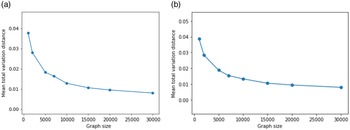
In Figure 1 we plot the mean of the total variation distance (4.1) averaged over 100 Monte Carlo simulations with $m=1$ and $\epsilon\sim U(0,\,1)$ for different graph sizes. Since our result is quenched in the fitness, we are keeping the same realization of the fitnesses and averaging the total variation distance over the Monte Carlo trials.

Figure 1.

(a) Mean of the total variation distance (4.1), $m=1$ , $\epsilon\sim U(0,\,1)$ . (b) Mean of the total variation distance (4.1), $m=5$ , $\epsilon\sim U(0,\,1)$ . Note that it decreases towards zero.

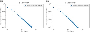
Due to the convergence of (4.1) we are also conjecturing that the asymptotic survival function of the degree distribution is close to a power law with exponent $\tau=2$ , as in the standard Barabási–Albert model [Reference van der Hofstad25, Section 8.4]. We then compare the tail exponent of the survival function of the degree distribution between our model in R1 and the Barabási–Albert model in Figure 2.

Figure 2.

Log-log plot of the empirical survival function for our model (a) in regime R1, $m=1$ , $\epsilon\sim \textrm{Beta}(1,\,3)$ , and a Barabási–Albert model (b). The plot looks like a straight line, which hints at a power-law behavior [Reference Cirillo9]. On top $\tau$ is computed.

Conjecture 4.2. (Convergence of the degree distribution in R2.) Let $m\in\mathbb{N}$ , and let $\textrm{deg}_t$ be the empirical degree distribution of a graph $G_t$ in regime R $2$ . Let $\textrm{deg}_t^{\textrm{BB}(m)}$ be the empirical degree distribution of a $\textrm{BB}(m)$ model with the same parameter $m\in\mathbb{N}$ . Then

(4.2) \begin{equation}\lim_{t\to\infty}d_{TV}\bigl(\textrm{deg}_t,\,\textrm{deg}_t^{\textrm{BB}(m)}\bigr)=0.\end{equation}

The limit is taken a.s. in the fitness realization of $G_t$ .

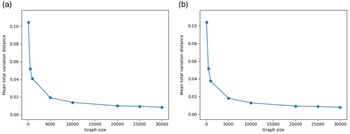
In Figure 3 we plot the mean total variation distance (4.2) over 100 Monte Carlo simulations with $m=5$ resp. $m=10$ and $\epsilon\sim \textrm{Beta}(1,\,3)$ for various graph sizes. As in the Barabási–Albert case, the fitness realization is kept fixed over the various Monte Carlo trials.

Figure 3.

(a) Mean of the total variation distance (4.2) between our model in regime R2 and $\textrm{BB}(m)$ , $m=5$ , $\epsilon\sim \textrm{Beta}(1,\,3)$ . (b) Mean of the total variation distance (4.2) between our model in regime R2 and $\textrm{BB}(m)$ , $m=10$ , $\epsilon\sim \textrm{Beta}(1,\,3)$ . In both cases it goes to zero.

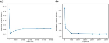
As a comparison, observe in Figure 4 the behavior of the mean total variation distance between our model in regime R2 with $m\neq 1$ and $\textrm{BB}(1)$ averaged over 100 Monte Carlo simulations. Again this hints at the fact that the way in which fitnesses increase does not substantially influence the growth of the network, provided we sum finitely many increments. This also shows that the $\textrm{BB}(m)$ model is robust under dynamical perturbations.

Figure 4.

(a) Mean total variation distance (4.2) between our model with $m=5$ and $\textrm{BB}(1)$ , $\epsilon\sim \textrm{Beta}(1,\,3).$ (b) Mean total variation distance (4.2) between our model with $m=2$ and $\textrm{BB}(1)$ , $\epsilon\sim U(0,\,1).$ In both cases the mean total variation does not approach zero.

4.2. Condensation

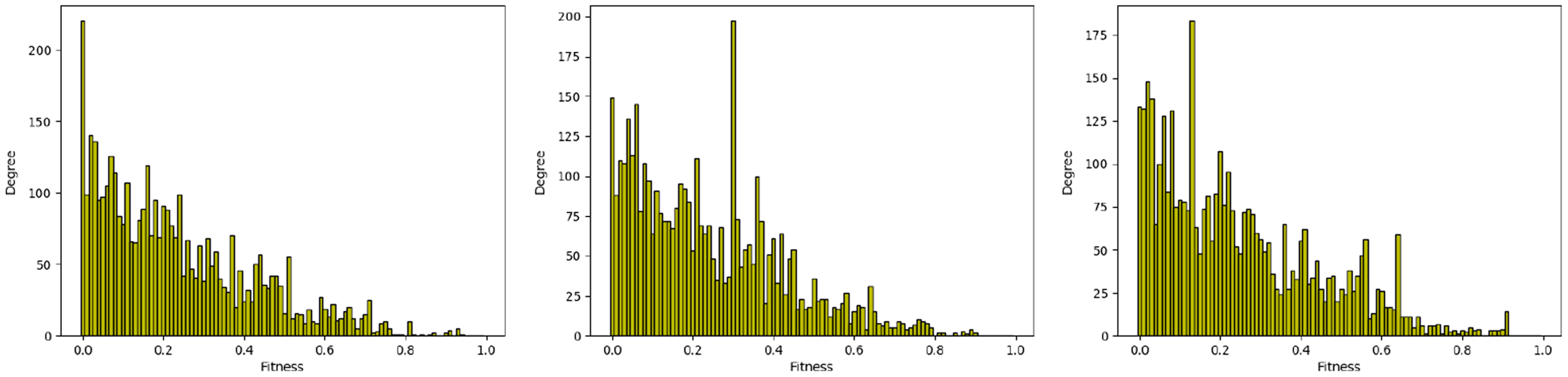
We now present the numerical results on condensation in regimes R1–R3. To do so, we will plot the cumulative degree of the nodes grouped by fitness. In this setting, based on the argument outlined in the Introduction, we expect to see condensation when the landscape of the above has more and higher spikes concentrated towards the upper end-point of the fitness law.

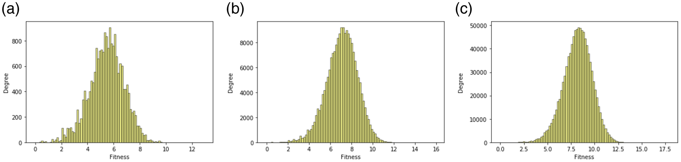
To begin with, recall that by Theorem 2.1 no condensate appears in regime R1. Indeed, when picturing condensation using the cumulative degree grouped by fitness (see Figure 5), one can see that the position of the spikes varies on the whole support of the distribution. This is due to the the m-Markov property.

Figure 5.

Cumulative degree of the nodes grouped by fitness for our model in regime R1 with $m=1$ , $\epsilon\sim \textrm{Beta}(1,\,3)$ . Observe that the location of the highest spike of the degree does not escape towards the supremum of the fitness but is randomly shuffled.

We now turn our attention to regimes R2 and R3.

4.3. Condensation for R2

Given Conjecture 4.2 on the asymptotic degree distribution, we formulate a conjecture on the condensation for R2 models.

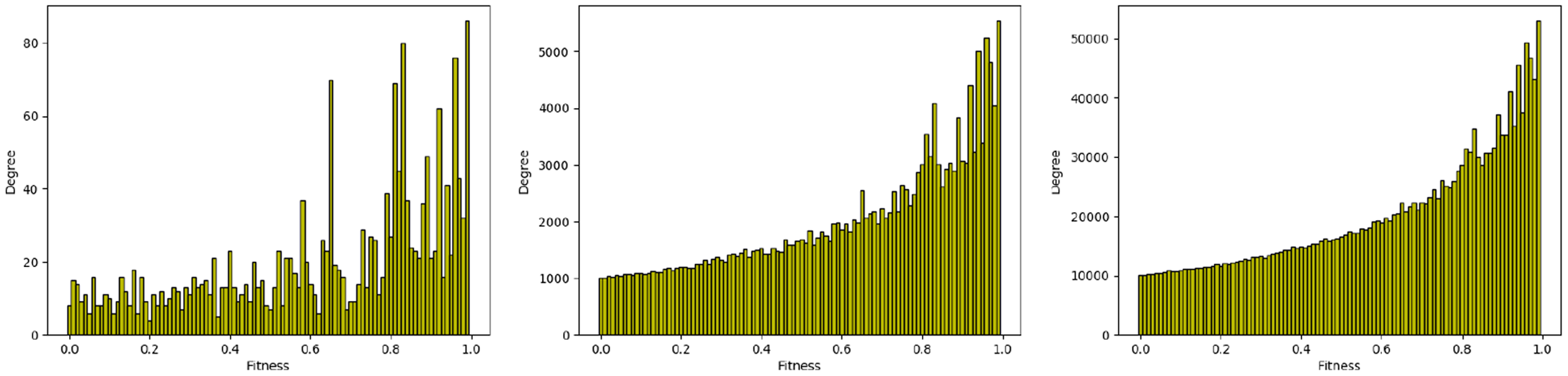
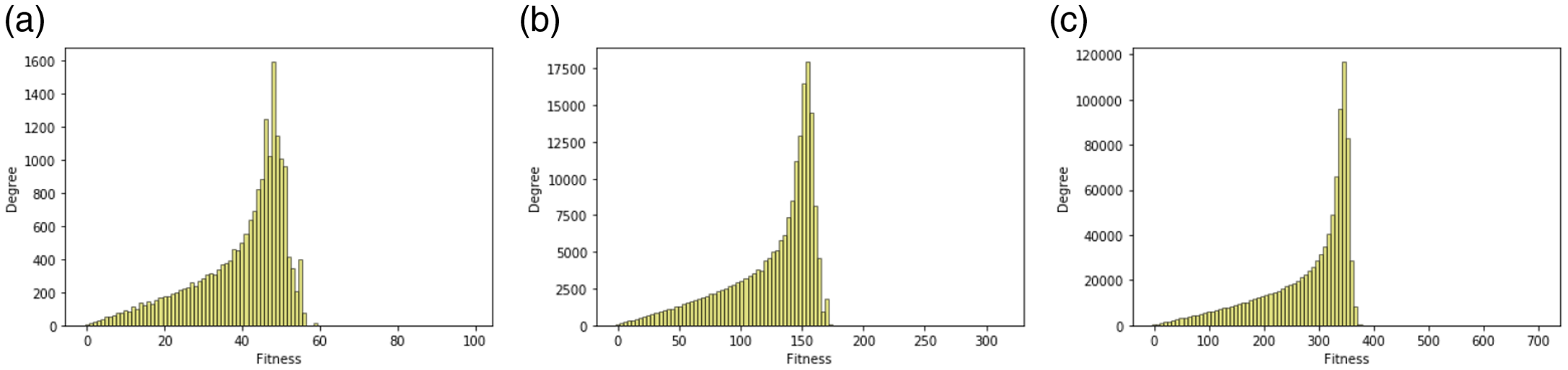
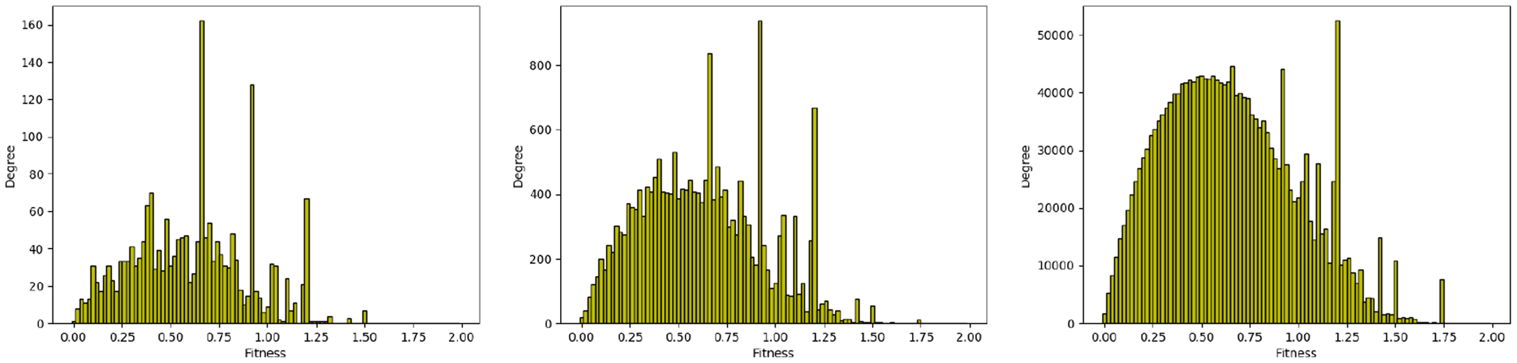
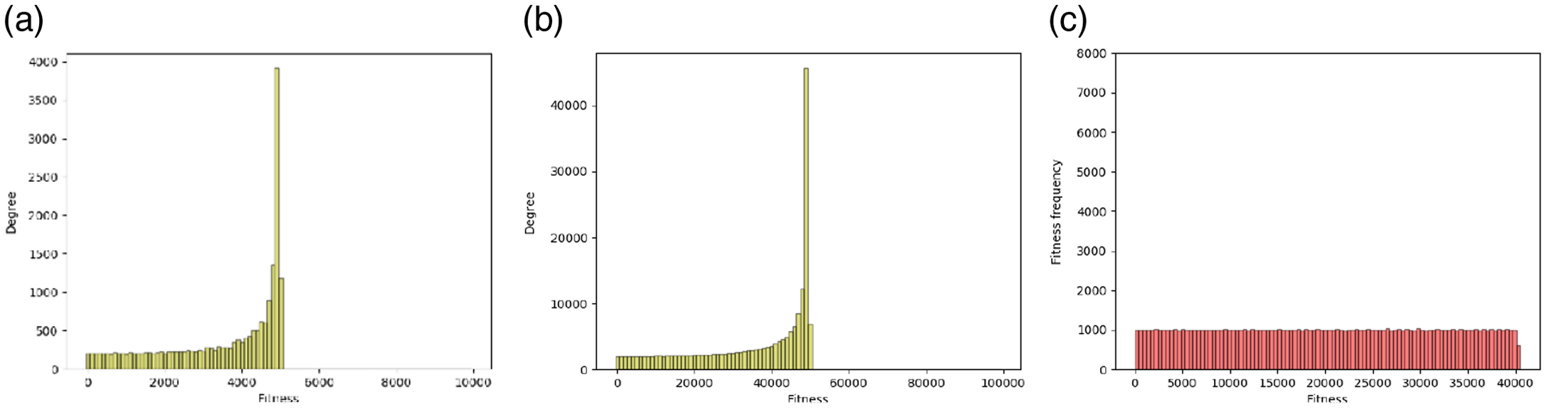
We will support the above conjecture with a few simulations. We recall [Reference Borgs, Chayes, Daskalakis and Roch8, Appendix C.3] that in a $\textrm{BB}(1)$ model the fitness distribution $\textrm{Beta}(\alpha,\,\beta)$ condensates if and only if $\beta>\alpha+1$ . In Figure 6 one can observe the absence of a condensate for $U(0,\,1)$ -distributed increments and $m=1$ . In Figure 7 a condensate appears for the increment distribution $\textrm{Beta}(1,\,1.9)$ when $m=2$ . 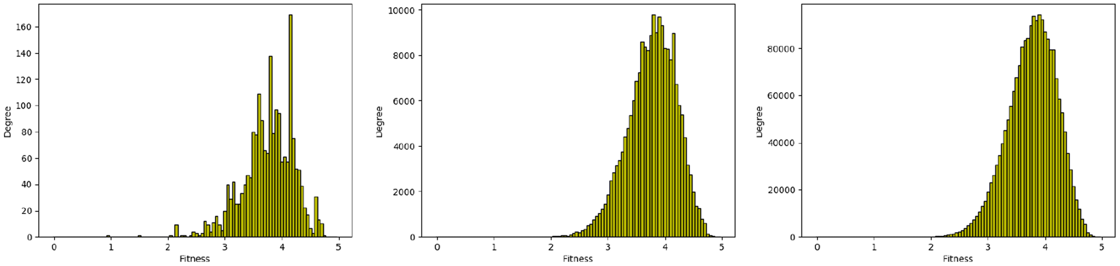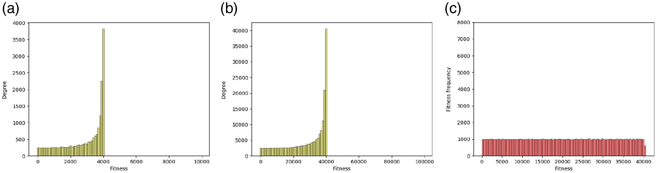Note finally in Figure 8 that there is no condensation for $\textrm{Beta}(3,\,1)$ -distributed increments for $m=5$ . Since in this case $\mu_\epsilon=\frac34>\frac12$ , the threshold in Proposition 2.1 seems to be binding in R2 as well.

Figure 6.

Cumulative degree in fitness intervals for regime R2 with $m=1$ , $\epsilon\sim U(0,\,1)$ . Note that the degree distribution per fitness becomes smoother at the right end-point of the fitness distribution. This model is known not to exhibit condensation.

Figure 7.

Cumulative degree in fitness intervals for regime R2 with $m=2$ with $\epsilon\sim \textrm{Beta}(1,\,1.9)$ . In this case higher spikes appear as the graph size increases towards the upper end-point of the fitness distribution. Recall that the classical Bianconi–Barabási model does not condensate for $\textrm{Beta}(1,\,1.9)$ -distributed fitness.

Figure 8.

Cumulative degree in fitness intervals for regime R2 with $m=5$ , $\epsilon\sim \textrm{Beta}(3,\,1)$ . The degree distribution per fitness appears without peaks as the graph increases and no condensates forms.

4.4. Condensation in regime R3

The case in which $m(t)\gg 1$ presents an interesting open problem which is illustrated in the following simulations.

In Figures 9–11 we plot the cumulative degree for nodes grouped by fitness with $U(0,\,1)$ increments in the regimes $m=\lfloor{\log t}\rfloor,\,\lfloor{\sqrt t}\rfloor,\,t$ respectively. As one can see, the limiting fitness distribution resembles the cumulative fitness distribution for the first two cases, while in the $m=t$ regime a spike appears at $\mu_\epsilon t$ .

Figure 9.

Cumulative degree grouped by fitness in regime R3 with $m=\lfloor{\log_2{t}}\rfloor$ with $\epsilon\sim U(0,\,1)$ . (c) Empirical fitness distribution corresponding to the last cumulative degree plot. Note that the empirical fitness distribution resembles the cumulative degree by fitness. The plots exhibit no spike.

Figure 10.

Cumulative degree grouped by fitness in regime R3 with $m=\lfloor{\sqrt t}\rfloor$ with $\epsilon\sim U(0,\,1)$ . (c) Empirical fitness distribution corresponding to the last cumulative degree plot. Note that the empirical fitness distribution resembles the cumulative degree by fitness. The plots exhibit no spike.

Figure 11.

Cumulative degree grouped by fitness in regime R3 with $m=t$ with $\epsilon\sim U(0,\,1)$ . (c) Empirical fitness distribution corresponding to the last cumulative degree plot. As expected, the fitness distribution is uniform in $[0,\,\mu_\epsilon t]$ . In particular $\mu_\epsilon=1/2,$ $t=100\,000$ , and $\mu_\epsilon t\approx 50\,000.$

As stated at the beginning of Section 4.2, in these kinds of plots condensation is indicated by the presence of spikes around the supremum of the fitness. Looking at Figures 9–10, there are no peaks and the landscape of the empirical fitness distribution resembles the cumulative degree grouped by fitness. On the other hand, in Figure 11 the two quantities are different: the cumulative degree by fitness exhibits a spike roughly around $\mu_\epsilon t$ , $t=100\,000$ , and the empirical fitness distribution seems to be uniform in $[0,\,\mu_\epsilon t].$ Heuristically, a uniform law appears because by summing a linear number of increments the central limit theorem kicks in, so that each node has roughly a Gaussian fitness. More precisely, for most nodes i the fitness is close in law to $\mathcal N(\mu_\epsilon (t-i),\sigma^2_\epsilon(t-i))$ , where $\sigma^2_\epsilon$ is the variance of the increments. Therefore, by Gaussian concentration properties around the mean, we see a fitness landscape close to uniform in $[0,\,\mu_\epsilon t].$

Based on the above considerations, we expect that the speed at which m(t) grows in time influences the appearance of a condensate. Namely, if m(t) is too slow, condensation cannot be enforced, while a faster m(t) leads to Bose–Einstein condensation. Because of the scaling of the central limit theorem, we conjecture $m(t)=\Theta( t)$ to be the threshold for condensation in R3.

This is summarized in the following conjecture.

We expect our results to be universal regardless of the increment distribution. In order to address this topic properly, we need to identify two fitness families. Mailler, Mörters, and Senkevich [Reference Mailler, Mörters and Senkevich22] proposed two fitness categories in the context of competing growth processes and dynamical networks. The difference arises essentially in the behavior at the maximal fitness value (regular variation vs. exponential behavior), which implies different treatment of the two regarding condensation. The families are:

1. (i) bounded random variables in the maximum domain of attraction of the Weibull distribution, e.g. Beta distribution [Reference Embrechts, Klüppelberg and Mikosch13, Section 3.3.2];

2. (ii) bounded random variables in the maximum domain of attraction of the Gumbel distribution, e.g. those with survival function [Reference Embrechts, Klüppelberg and Mikosch13, Section 3.3.3], that is,

   (4.3) \begin{equation}\overline F(x)=\exp\!({-}x/(1-x)),\quad x\in[0,\,1].\end{equation}

So far we have used Beta-distributed increments in our simulations. In order to better support our claims, we provide a realization of our model in R3 with increments belonging to class (ii). Namely, we will use increments distributed as (4.3). As one can see, the behavior shown in Figure 12 is qualitatively similar to Figure 11. The intuition behind this is that the central limit theorem works regardless of the initial increment distribution.

Figure 12.

Cumulative degree grouped by fitness in regime R3 with $m=t$ with increments distributed as (4.3). (c) Empirical fitness distribution corresponding to the last cumulative degree plot. As expected, the fitness distribution is uniform in $[0,\,\mu_\epsilon t]$ . In particular $\mu_\epsilon=1/2$ , $t=100\,000$ , and $\mu_\epsilon t\approx 50\,000.$