1 Introduction
Systems with flow coupled to heat transfer, mass transfer or reactions can exhibit oscillations when spatial variations in temperature or composition create non-uniform surface tensions. Examples of such oscillatory systems include the periodic ejection of fine droplets from a pendant water drop in oil (Fernandez & Homsy Reference Fernandez and Homsy2004), the beating of an oil lens on water (Stocker & Bush Reference Stocker and Bush2007) and the intermittent flow of a free water surface due to diffusion of an organic molecule from a droplet below the surface (Kovalchuk et al. Reference Kovalchuk, Kamusewitz, Vollhardt and Kovalchuk1999). The time scales of the oscillations range from several tenths of a second in the first two examples to minutes in the third example. In all of these systems, the flows are driven by spatial variations in the concentration of surface active molecules (surfactants), and therefore also surface tension, along a surface. In general, flows driven by spatially varying surface tension are referred to as Marangoni flows, and they occur in many natural phenomena and industrial processes (Scriven & Sternling Reference Scriven and Sternling1960). In this paper, we study the spreading of surfactants on a free surface and find that oscillations also occur in this simpler system.
When surfactants are deposited on the free surface of a liquid, they typically locally reduce the surface tension, driving a flow that spreads the surfactant over the surface. The spreading of surfactants used to treat surfactant deficiency in the lungs of prematurely born infants (Grotberg Reference Grotberg1994) motivated early studies of spreading on thin films (Jensen & Grotberg Reference Jensen and Grotberg1992; Jensen Reference Jensen1994). Such spreading flows on thin films can develop fingering instabilities (Troian, Herbolzheimer & Safran Reference Troian, Herbolzheimer and Safran1990; Matar & Troian Reference Matar and Troian1999; Edmonstone, Craster & Matar Reference Edmonstone, Craster and Matar2006; Jensen & Naire Reference Jensen and Naire2006). In addition, surfactant spreading on deep fluid layers has been studied (Jensen Reference Jensen1995; Thess Reference Thess1996; Dussaud & Troian Reference Dussaud and Troian1998).
Interest in Marangoni flows has also been driven by their role in the motion of particles (Pimienta & Antoine Reference Pimienta and Antoine2014) and organisms (Bush & Hu Reference Bush and Hu2006) along interfaces. A classic example of particle motion is the erratic movement of camphor when it is placed on water (Rayleigh Reference Rayleigh1890; Nakata et al.
Reference Nakata, Iguchi, Ose, Kuboyama, Ishii and Yoshikawa1997; Nakata & Hayashima Reference Nakata and Hayashima1998). This motion occurs due to gradients in surface tension around the particles that are created by non-uniform spreading of camphor molecules, which act as a surfactant. These systems are interesting from a thermodynamic perspective because chemical energy is converted to kinetic energy in the absence of a temperature gradient (Nakata et al.
Reference Nakata, Iguchi, Ose, Kuboyama, Ishii and Yoshikawa1997). Such isothermal conversion of chemical to kinetic energy also occurs in biological locomotion, in contrast to the large temperature differences required by heat engines. In fact, some organisms directly exploit Marangoni flows for propulsion (Bush & Hu Reference Bush and Hu2006). For example, the water-walking insects Microvelia can reach speeds of
 $17~\text{cm}~\text{s}^{-1}$
, which is twice their walking speed, by releasing a surfactant.
In addition to driving the motion of individual particles at interfaces, spatial variations in surfactant concentration and surface tension are responsible for coupling the motion of several particles (Kohira et al. Reference Kohira, Hayashima, Nagayama and Nakata2001; Nakata, Doi & Kitahata Reference Nakata, Doi and Kitahata2005). For individual particles, the speeds of disks (Lauga & Davis Reference Lauga and Davis2012) and spheroids (Masoud & Stone Reference Masoud and Stone2014) that asymmetrically release insoluble surfactants have been determined. The collective motion of particles on an interface that locally increase surface tension by reacting with a surface active compound in the adjacent fluid layer has also been studied. Such particles aggregate due to the higher tension in regions of the surface with a higher particle concentration. The possibility of a collapse of particle distributions to points in finite time has been demonstrated (Masoud & Shelley Reference Masoud and Shelley2014), but the effects of inertia were not considered.
Here, we consider the spreading of an insoluble surfactant, which reduces surface tension, on a deep layer of Newtonian fluid that is initially motionless. For unsteady Stokes flow (the appropriate linearized version of the Navier–Stokes equations) with sufficient inertia (i.e. an appropriately defined Reynolds number exceeds a critical value), we find that sinusoidal spatial variations in surfactant concentration oscillate as they decay in time to a uniform distribution. Such longitudinal surface oscillations are distinct from longitudinal waves due to surface elasticity (Lucassen Reference Lucassen1968a ,Reference Lucassen b ) and interfacial instability during transfer of a soluble surfactant across an interface (Sternling & Scriven Reference Sternling and Scriven1959; Velarde & Chu Reference Velarde and Chu1989). In § 2, we present the coupled initial value problem for surfactant spreading and flow. We derive, in § 3, solutions to this problem for the limit of small-amplitude variations in surfactant concentration and negligible surfactant diffusion. In this limit, the flow and surfactant transport equations are linear, and solutions are provided for both the limits of quasi-steady Stokes flow and unsteady Stokes flow of the fluid. Nonlinear surfactant spreading and fluid flow due to initial concentration variations with finite amplitude are studied numerically in § 4 and compared with the behaviour in the linear limit.
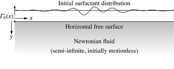
Schematic of the modelled system. An arbitrary initial distribution of insoluble surfactant
 $\unicode[STIX]{x1D6E4}_{0}(x)$
drives the incompressible flow of a semi-infinite layer of Newtonian fluid, which redistributes the surfactant.

2 Problem definition
Consider the transport of an insoluble surfactant along the free surface of a semi-infinite fluid domain in two dimensions, as illustrated in figure 1. Let the
 $x$
axis be parallel to the fluid surface, which is assumed to remain flat, and
 $y$
be perpendicular to it and extend into the fluid. The surface is therefore located at
 $y=0$
, and fluid is present in the half-plane
 $y\in [0,\infty )$
. The surface concentration of the surfactant
 $\unicode[STIX]{x1D6E4}(x,t)$
evolves according to the advection–diffusion equation
 $$\begin{eqnarray}\frac{\unicode[STIX]{x2202}\unicode[STIX]{x1D6E4}}{\unicode[STIX]{x2202}t}+\frac{\unicode[STIX]{x2202}}{\unicode[STIX]{x2202}x}(\unicode[STIX]{x1D6E4}u_{s})=D_{s}\frac{\unicode[STIX]{x2202}^{2}\unicode[STIX]{x1D6E4}}{\unicode[STIX]{x2202}x^{2}},\end{eqnarray}$$
where
 $u_{s}$
is the
 $x$
component of the fluid velocity
 $\boldsymbol{u}=(u,v)$
at
 $y=0$
and
 $D_{s}$
is the diffusivity of the surfactant along the surface. The surfactant concentration determines the surface tension
 $\unicode[STIX]{x1D6FE}$
through the linear equation of state
 $$\begin{eqnarray}\unicode[STIX]{x1D6FE}=\unicode[STIX]{x1D6FE}_{0}-\unicode[STIX]{x1D6FC}\unicode[STIX]{x1D6E4},\end{eqnarray}$$
where
 $\unicode[STIX]{x1D6FE}_{0}$
is the tension of a surfactant-free surface and
 $\unicode[STIX]{x1D6FC}$
is the proportionality constant. This simplification is common and used widely in the literature. It follows that the mean surface tension
 $\bar{\unicode[STIX]{x1D6FE}}$
on a surface is
 $\unicode[STIX]{x1D6FE}_{0}-\unicode[STIX]{x1D6FC}\bar{\unicode[STIX]{x1D6E4}}$
, where
 $\bar{\unicode[STIX]{x1D6E4}}$
is the mean surfactant concentration. We restrict our attention to the case of a surfactant that reduces surface tension, i.e.
 $\unicode[STIX]{x1D6FC}>0$
. We assume that the bulk fluid is Newtonian with dynamic viscosity
 $\unicode[STIX]{x1D707}$
and density
 $\unicode[STIX]{x1D70C}$
, and the flow is incompressible. The fluid velocity
 $\boldsymbol{u}(x,y,t)$
and pressure
 $p(x,y,t)$
therefore evolve according to
 $$\begin{eqnarray}\unicode[STIX]{x1D70C}\left(\frac{\unicode[STIX]{x2202}\boldsymbol{u}}{\unicode[STIX]{x2202}t}+\boldsymbol{u}\boldsymbol{\cdot }\unicode[STIX]{x1D735}\boldsymbol{u}\right)=-\unicode[STIX]{x1D735}p+\unicode[STIX]{x1D707}\unicode[STIX]{x1D6FB}^{2}\boldsymbol{u}\end{eqnarray}$$
together with the continuity equation
 $$\begin{eqnarray}\unicode[STIX]{x1D735}\boldsymbol{\cdot }\boldsymbol{u}=0.\end{eqnarray}$$
Variations in surface tension along the surface of the fluid (at
 $y=0$
) impose a Marangoni stress on it, which leads to the boundary condition
 $$\begin{eqnarray}\left.\frac{\unicode[STIX]{x2202}u}{\unicode[STIX]{x2202}y}\right|_{y=0}=-\frac{1}{\unicode[STIX]{x1D707}}\frac{\unicode[STIX]{x2202}\unicode[STIX]{x1D6FE}}{\unicode[STIX]{x2202}x}=\frac{\unicode[STIX]{x1D6FC}}{\unicode[STIX]{x1D707}}\frac{\unicode[STIX]{x2202}\unicode[STIX]{x1D6E4}}{\unicode[STIX]{x2202}x}.\end{eqnarray}$$
We consider the initial value problem of a given surfactant distribution on an initially motionless fluid and determine how the surfactant distribution and flow evolve over time. This problem has the initial conditions
 $$\begin{eqnarray}\unicode[STIX]{x1D6E4}(x,0)=\unicode[STIX]{x1D6E4}_{0}(x),\quad \boldsymbol{u}(x,y,0)=\mathbf{0}\end{eqnarray}$$
and the boundary conditions are (2.5) together with
 $$\begin{eqnarray}v(x,0,t)=0,\quad |\boldsymbol{u}|=0\quad \text{as }y\rightarrow \infty ,\quad p=0\quad \text{as }y\rightarrow \infty ,\end{eqnarray}$$
for
 $t>0$
. The ambient constant pressure is a reference that is set equal to zero. The first boundary condition arises from the assumption of a flat interface. While the normal component of the velocity is zero along the surface, the tangential component varies due to the non-uniform surfactant concentration and stress.
We now non-dimensionalize the governing equations, using the idea that there is a Marangoni flow driven by small deviations in the surfactant concentration about a mean value. We start with the Marangoni surface stress, equation (2.5), that provides the characteristic speed of the system. We proceed by introducing
 $\tilde{x}=x/\unicode[STIX]{x1D706}$
,
 ${\tilde{y}}=y/\unicode[STIX]{x1D706}$
,
 $\tilde{u} =u/\unicode[STIX]{x1D700}u^{\ast }$
, and
 $\tilde{\unicode[STIX]{x1D6E4}}=(\unicode[STIX]{x1D6E4}-\bar{\unicode[STIX]{x1D6E4}})/(\unicode[STIX]{x1D700}\bar{\unicode[STIX]{x1D6E4}})$
, where the length scale
 $\unicode[STIX]{x1D706}$
, mean surfactant concentration
 $\bar{\unicode[STIX]{x1D6E4}}$
and amplitude of the variation in surfactant concentration
 $\unicode[STIX]{x1D700}\bar{\unicode[STIX]{x1D6E4}}$
are all properties of the initial surfactant distribution. Choosing
 $u^{\ast }=\unicode[STIX]{x1D6FC}\bar{\unicode[STIX]{x1D6E4}}/\unicode[STIX]{x1D707}$
, we are left with
 $$\begin{eqnarray}\left.\frac{\unicode[STIX]{x2202}\tilde{u} }{\unicode[STIX]{x2202}{\tilde{y}}}\right|_{{\tilde{y}}=0}=\frac{\unicode[STIX]{x2202}\tilde{\unicode[STIX]{x1D6E4}}}{\unicode[STIX]{x2202}\tilde{x}}.\end{eqnarray}$$
Recalling the relationship between the surface tension and surfactant concentration, equation (2.2), we see that
 $\unicode[STIX]{x1D700}\unicode[STIX]{x1D6FC}\bar{\unicode[STIX]{x1D6E4}}$
is the amplitude of the variation in surface tension. Therefore,
 $\unicode[STIX]{x1D700}u^{\ast }$
can be interpreted as a Marangoni speed, the ratio of the surface tension difference that drives flow and the resisting viscous stress.
Next, the surfactant advection–diffusion equation (2.1) becomes
 $$\begin{eqnarray}\frac{\unicode[STIX]{x2202}\tilde{\unicode[STIX]{x1D6E4}}}{\unicode[STIX]{x2202}\tilde{t}}+\unicode[STIX]{x1D700}\frac{\unicode[STIX]{x2202}}{\unicode[STIX]{x2202}\tilde{x}}(\tilde{\unicode[STIX]{x1D6E4}}\tilde{u} _{s})+\frac{\unicode[STIX]{x2202}\tilde{u} _{s}}{\unicode[STIX]{x2202}\tilde{x}}=\mathit{Pe}_{s}^{-1}\frac{\unicode[STIX]{x2202}^{2}\tilde{\unicode[STIX]{x1D6E4}}}{\unicode[STIX]{x2202}\tilde{x}^{2}},\end{eqnarray}$$
where
 $\tilde{u} _{s}=u_{s}/(\unicode[STIX]{x1D700}u^{\ast })$
,
 $\tilde{t}=t/t^{\ast }$
, and
 $t^{\ast }=\unicode[STIX]{x1D706}/u^{\ast }$
is an advective time scale. The Péclet number
 $\mathit{Pe}_{s}=u^{\ast }\unicode[STIX]{x1D706}/D_{s}$
is the ratio of the diffusive time scale
 $\unicode[STIX]{x1D706}^{2}/D_{s}$
and the advective time scale
 $\unicode[STIX]{x1D706}/u^{\ast }$
. Using this scaling together with
 $\tilde{p}=p\unicode[STIX]{x1D706}/(\unicode[STIX]{x1D700}\unicode[STIX]{x1D707}u^{\ast })$
, the Navier–Stokes and continuity equations become
 $$\begin{eqnarray}\mathit{Re}\left(\frac{\unicode[STIX]{x2202}\tilde{\boldsymbol{u}}}{\unicode[STIX]{x2202}\tilde{t}}+\unicode[STIX]{x1D700}\tilde{\boldsymbol{u}}\boldsymbol{\cdot }\tilde{\unicode[STIX]{x1D735}}\tilde{\boldsymbol{u}}\right)=-\tilde{\unicode[STIX]{x1D735}}\tilde{p}+\tilde{\unicode[STIX]{x1D6FB}}^{2}\tilde{\boldsymbol{u}}\end{eqnarray}$$
and
 $$\begin{eqnarray}\tilde{\unicode[STIX]{x1D735}}\boldsymbol{\cdot }\tilde{\boldsymbol{u}}=0,\end{eqnarray}$$
where
 $\tilde{\boldsymbol{u}}=\boldsymbol{u}/(\unicode[STIX]{x1D700}u^{\ast })$
. The Reynolds number is defined according to
 $\mathit{Re}=\unicode[STIX]{x1D70C}u^{\ast }\unicode[STIX]{x1D706}/\unicode[STIX]{x1D707}=\unicode[STIX]{x1D70C}\unicode[STIX]{x1D6FC}\bar{\unicode[STIX]{x1D6E4}}\unicode[STIX]{x1D706}/\unicode[STIX]{x1D707}^{2}=\unicode[STIX]{x1D70C}(\unicode[STIX]{x1D6FE}_{0}-\bar{\unicode[STIX]{x1D6FE}})\unicode[STIX]{x1D706}/\unicode[STIX]{x1D707}^{2}$
.
In non-dimensional form, we seek the solution to equations (2.9), (2.10) and (2.11) with the initial conditions
 $$\begin{eqnarray}\tilde{\unicode[STIX]{x1D6E4}}(\tilde{x},0)=\tilde{\unicode[STIX]{x1D6E4}}_{0}(\tilde{x}),\quad \tilde{\boldsymbol{u}}(\tilde{x},{\tilde{y}},0)=\mathbf{0}\end{eqnarray}$$
and the boundary conditions
 $$\begin{eqnarray}\tilde{v}(\tilde{x},0,\tilde{t})=0,\quad \left.\frac{\unicode[STIX]{x2202}\tilde{u} }{\unicode[STIX]{x2202}{\tilde{y}}}\right|_{{\tilde{y}}=0}=\frac{\unicode[STIX]{x2202}\tilde{\unicode[STIX]{x1D6E4}}}{\unicode[STIX]{x2202}\tilde{x}},\quad |\tilde{\boldsymbol{u}}|=0\quad \text{as }{\tilde{y}}\rightarrow \infty ,\quad \text{and}\quad \tilde{p}=0\quad \text{as }{\tilde{y}}\rightarrow \infty .\end{eqnarray}$$
3 Analytical solutions
In the limit of low
 $\mathit{Pe}_{s}$
, we expect smoothing of the surfactant distribution due to diffusion without significant motion of the underlying fluid. The case of high
 $\mathit{Pe}_{s}$
is more interesting and relevant to physical systems, and we now pursue analytical solutions for the limit
 $\mathit{Pe}_{s}\rightarrow \infty$
. We further consider the limit of small variations in surfactant concentration relative to the average concentration, i.e.
 $\unicode[STIX]{x1D700}\rightarrow 0$
. This limit has two effects on the governing equations: the nonlinear terms vanish in both the surfactant and flow equations, (2.9) and (2.10) respectively, leaving the linear system
 $$\begin{eqnarray}\displaystyle & \displaystyle \frac{\unicode[STIX]{x2202}\tilde{\unicode[STIX]{x1D6E4}}}{\unicode[STIX]{x2202}\tilde{t}}+\frac{\unicode[STIX]{x2202}\tilde{u} _{s}}{\unicode[STIX]{x2202}\tilde{x}}=0, & \displaystyle\end{eqnarray}$$
 $$\begin{eqnarray}\displaystyle & \displaystyle \mathit{Re}\frac{\unicode[STIX]{x2202}\tilde{\boldsymbol{u}}}{\unicode[STIX]{x2202}\tilde{t}}=-\tilde{\unicode[STIX]{x1D735}}\tilde{p}+\tilde{\unicode[STIX]{x1D6FB}}^{2}\tilde{\boldsymbol{u}}, & \displaystyle\end{eqnarray}$$
 $$\begin{eqnarray}\displaystyle & \displaystyle \tilde{\unicode[STIX]{x1D735}}\boldsymbol{\cdot }\tilde{\boldsymbol{u}}=0. & \displaystyle\end{eqnarray}$$
 $\unicode[STIX]{x2202}\tilde{u} _{s}/\unicode[STIX]{x2202}\tilde{x}$
along the surface), and changes in surfactant concentration therefore occur due to expansion or contraction of the surface.
We now proceed to find the solution for this linear initial value problem, first making no assumptions about the form of the initial surfactant distribution, i.e. letting
 $\tilde{\unicode[STIX]{x1D6E4}}_{0}(\tilde{x})$
be arbitrary. Additional details about the derivation are provided in appendix B. Since we make frequent use of Fourier (
 $\mathscr{F}$
) transforms with respect to
 $\tilde{x}$
, Laplace (
 $\mathscr{L}$
) transforms with respect to
 $\tilde{t}$
, and their inverses, we use the notation
 $$\begin{eqnarray}\displaystyle & \displaystyle \hat{p}(k,{\tilde{y}},\tilde{t})=\mathscr{F}\{p(\tilde{x},{\tilde{y}},\tilde{t})\}\;\Longleftrightarrow \;p(\tilde{x},{\tilde{y}},\tilde{t})=\mathscr{F}^{-1}\{\hat{p}(k,{\tilde{y}},\tilde{t})\}, & \displaystyle\end{eqnarray}$$
 $$\begin{eqnarray}\displaystyle & \displaystyle \breve{p}(k,{\tilde{y}},s)=\mathscr{L}\{\hat{p}(k,{\tilde{y}},\tilde{t})\}\;\Longleftrightarrow \;\hat{p}(k,{\tilde{y}},\tilde{t})=\mathscr{L}^{-1}\{\breve{p}(k,{\tilde{y}},s)\} & \displaystyle\end{eqnarray}$$
 $k$
is the wavenumber and
 $s$
is the complex frequency. We take the divergence of (3.1b
) and a Fourier transform in
 $\tilde{x}$
to obtain
 $$\begin{eqnarray}-k^{2}\hat{p}+\frac{\unicode[STIX]{x2202}^{2}\hat{p}}{\unicode[STIX]{x2202}{\tilde{y}}^{2}}=0.\end{eqnarray}$$
Ensuring boundedness as
 ${\tilde{y}}\rightarrow \infty$
, the solution for the pressure is
 $$\begin{eqnarray}\hat{p}(k,{\tilde{y}},\tilde{t})=\hat{p}_{0}(k,\tilde{t})\exp (-|k|{\tilde{y}}),\quad \breve{p}(k,{\tilde{y}},s)=\breve{p}_{0}(k,s)\exp (-|k|{\tilde{y}}),\end{eqnarray}$$
where
 $\hat{p}_{0}(k,\tilde{t})$
is the pressure at the surface and remains to be determined. Now, taking the Fourier and Laplace transforms of the
 ${\tilde{y}}$
component of the momentum equation (3.1b
) yields
 $$\begin{eqnarray}(\mathit{Re}\,s+k^{2})\breve{v}-\frac{\unicode[STIX]{x2202}^{2}\breve{v}}{\unicode[STIX]{x2202}{\tilde{y}}^{2}}=|k|\,\breve{p}_{0}(k,s)\exp (-|k|{\tilde{y}}).\end{eqnarray}$$
Retaining the terms that are bounded as
 ${\tilde{y}}\rightarrow \infty$
and using
 $\breve{v}=0$
at
 ${\tilde{y}}=0$
, the solution is
 $$\begin{eqnarray}\breve{v}(k,{\tilde{y}},s)=\frac{|k|\,\breve{p}_{0}(k,s)}{\mathit{Re}\,s}\left[\exp (-|k|{\tilde{y}})-\exp \left(-{\tilde{y}}\sqrt{k^{2}+\mathit{ Re }\,s}\right)\right].\end{eqnarray}$$
From the incompressibility constraint
 $\text{i}k\breve{u}+\unicode[STIX]{x2202}\breve{v}/\unicode[STIX]{x2202}{\tilde{y}}=0$
we find that
 $$\begin{eqnarray}\breve{u}(k,{\tilde{y}},s)=\frac{\text{i}k\,\breve{p}_{0}(k,s)}{|k|\mathit{Re}\,s}\left[\sqrt{k^{2}+\mathit{ Re }\,s}\exp \left(-{\tilde{y}}\sqrt{k^{2}+\mathit{ Re }\,s}\right)-|k|\exp (-|k|{\tilde{y}})\right].\end{eqnarray}$$
At the surface (
 ${\tilde{y}}=0$
), the solutions simplify to
 $$\begin{eqnarray}\displaystyle & \displaystyle \breve{u}(k,0,s)=\frac{\text{i}k}{|k|}\breve{p}_{0}(k,s)\frac{\sqrt{k^{2}+\mathit{Re }\,s}-|k|}{\mathit{Re}\,s}, & \displaystyle\end{eqnarray}$$
 $$\begin{eqnarray}\displaystyle & \displaystyle \breve{v}(k,0,s)=0, & \displaystyle\end{eqnarray}$$
 $$\begin{eqnarray}\displaystyle & \displaystyle \breve{p}(k,0,s)=\breve{p}_{0}(k,s). & \displaystyle\end{eqnarray}$$
 $$\begin{eqnarray}\breve{p}_{0}(k,s)=-|k|\,\breve{\unicode[STIX]{x1D6E4}}(k,s).\end{eqnarray}$$
3.1 Solution for a single mode
To this point, the derivation has considered an arbitrary initial surfactant distribution
 $\tilde{\unicode[STIX]{x1D6E4}}_{0}(\tilde{x})$
, and we now restrict our attention to a particular distribution: a single sinusoidal mode. Though a pure sinusoid is an unlikely initial condition for a physical system, the solution for any periodic initial condition can be expressed as a series of the solutions for individual modes due to the linearity of the governing system of equations. Furthermore, the solution for a pure sinusoid is useful because the fundamental mode decays slowest, as we will show, and therefore determines the late-time dynamics. Choosing the length scale
 $\unicode[STIX]{x1D706}$
to be the wavelength of the initial sinusoidal variation in the surfactant concentration, the initial distribution
 $\tilde{\unicode[STIX]{x1D6E4}}_{0}(\tilde{x})$
is
 $$\begin{eqnarray}\tilde{\unicode[STIX]{x1D6E4}}_{0}(\tilde{x})=\sin (2\unicode[STIX]{x03C0}\tilde{x}).\end{eqnarray}$$
We now take the Fourier and Laplace transforms of the surfactant evolution equation (3.1a ) to obtain
 $$\begin{eqnarray}s\breve{\unicode[STIX]{x1D6E4}}(k,s)-\hat{\unicode[STIX]{x1D6E4}}_{0}(k)+\text{i}k\breve{u}_{s}(k,s)=0,\end{eqnarray}$$
where
 $\breve{u}_{s}(k,s)=\breve{u}(k,0,s)$
and
 $\hat{\unicode[STIX]{x1D6E4}}_{0}(k)=\hat{\unicode[STIX]{x1D6E4}}(k,0)$
. Substituting (3.9a
) and (3.10), we arrive at the Laplace-domain solution for the surfactant evolution:
 $$\begin{eqnarray}\breve{\unicode[STIX]{x1D6E4}}(k,s)=\frac{1}{\displaystyle s+\frac{|k|^{3}}{\mathit{Re}\,s}\left(\sqrt{1+\frac{\mathit{ Re }\,s}{k^{2}}}-1\right)}\hat{\unicode[STIX]{x1D6E4}}_{0}(k).\end{eqnarray}$$
For the initial condition we are interested in, a single sinusoidal mode, we have
 $\hat{\unicode[STIX]{x1D6E4}}_{0}(k)=-\text{i}\unicode[STIX]{x03C0}\,\text{sgn}(k)\,\unicode[STIX]{x1D6FF}(|k|-2\unicode[STIX]{x03C0})$
, where
 $\unicode[STIX]{x1D6FF}(\cdot )$
is the Dirac delta function and
 $\text{sgn}(\cdot )$
is the sign function, and therefore need to only consider
 $|k|=2\unicode[STIX]{x03C0}$
. The resulting solution is
 $$\begin{eqnarray}\breve{\unicode[STIX]{x1D6E4}}(k,s)=\frac{-\text{i}\unicode[STIX]{x03C0}\,\text{sgn}(k)\,\unicode[STIX]{x1D6FF}(|k|-2\unicode[STIX]{x03C0})}{\displaystyle s+\frac{8\unicode[STIX]{x03C0}^{3}}{\mathit{Re}\,s}\left(\sqrt{1+\frac{\mathit{ Re }\,s}{4\unicode[STIX]{x03C0}^{2}}}-1\right)}.\end{eqnarray}$$
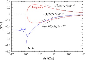
To gain first a qualitative understanding of the surfactant dynamics, we examine the poles of (3.14). As illustrated in figure 2, the dynamics can be classified into one of five cases depending on the value of the Reynolds number:


-
(i)
 $\mathit{Re}\rightarrow 0$
. In this limit, which describes dominantly viscous systems, the pole is
$s=-\unicode[STIX]{x03C0}$
. In the absence of the term on the left-hand side of (2.10), we have a Stokes flow. The complete solution for this case can be derived either directly from the governing equations or using the
$\mathit{Re}\rightarrow 0$
limit of the solutions that have already been derived, which we present in § 3.2. The Stokes flow solution for a two-dimensional surface and a finite fluid depth is also available (Masoud & Shelley Reference Masoud and Shelley2014).
-
(ii)
$\mathit{Re}/(2\unicode[STIX]{x03C0})<1$
, for which only one negative real pole exists. -
(iii)
$1<\mathit{Re}/(2\unicode[STIX]{x03C0})<32/27$
, for which two negative real poles exist. -
(iv)
$\mathit{Re}/(2\unicode[STIX]{x03C0})>32/27$
, for which two complex conjugate poles with negative real parts exist. -
(v)
$\mathit{Re}\gg 1$
. In this limit, equation (3.14) simplifies to (3.15)where
$$\begin{eqnarray}\breve{\unicode[STIX]{x1D6E4}}(k,s)=-\text{i}\unicode[STIX]{x03C0}\,\text{sgn}(k)\,\unicode[STIX]{x1D6FF}(|k|-2\unicode[STIX]{x03C0})\,\breve{\unicode[STIX]{x1D703}}(s),\end{eqnarray}$$
(3.16)and has the two poles
$$\begin{eqnarray}\breve{\unicode[STIX]{x1D703}}(s)=\frac{1}{\displaystyle s+\frac{4\unicode[STIX]{x03C0}^{2}}{\mathit{Re}^{1/2}s^{1/2}}}\end{eqnarray}$$
(3.17)The poles are complex conjugates of each other and have negative real parts. Both the real and imaginary parts of the two poles decay to zero in proportion to
$$\begin{eqnarray}s=2\unicode[STIX]{x03C0}\left(\frac{\mathit{Re}}{2\unicode[STIX]{x03C0}}\right)^{-1/3}\left(-\frac{1}{2}\pm \text{i}\frac{\sqrt{3}}{2}\right).\end{eqnarray}$$
$\mathit{Re}^{-1/3}$
.






We focus now on the limit of large
 $\mathit{Re}$
and invert the Laplace-domain solution, equation (3.15), back to the time domain. First, we note that
 $$\begin{eqnarray}\displaystyle \breve{\unicode[STIX]{x1D703}}(s) & = & \displaystyle \frac{1}{\displaystyle s+\frac{4\unicode[STIX]{x03C0}^{2}}{\mathit{Re}^{1/2}\,s^{1/2}}}\nonumber\\ \displaystyle & = & \displaystyle \frac{1}{3s^{1/2}}\left[{\displaystyle \frac{1}{s^{1/2}-b_{0}\frac{\displaystyle (2\unicode[STIX]{x03C0})^{2/3}}{\displaystyle \mathit{Re}^{1/6}}}}+{\displaystyle \frac{1}{s^{1/2}-b_{+}\frac{\displaystyle (2\unicode[STIX]{x03C0})^{2/3}}{\displaystyle \mathit{Re}^{1/6}}}}+{\displaystyle \frac{1}{s^{1/2}-b_{-}\frac{\displaystyle (2\unicode[STIX]{x03C0})^{2/3}}{\displaystyle \mathit{Re}^{1/6}}}}\right],\qquad\end{eqnarray}$$
where
 $b_{0}=-1$
and
 $b_{\pm }=(1\pm \text{i}\sqrt{3})/2$
are the three cube roots of
 $-1$
. Of the three terms on the right, the first does not contribute a pole. The inverse Laplace transform of
 $$\begin{eqnarray}F(s)=\frac{1}{\sqrt{s}\left(\sqrt{s}+\unicode[STIX]{x1D6FD}\right)},\end{eqnarray}$$
where
 $\unicode[STIX]{x1D6FD}$
is a complex constant, is (Erdélyi et al.
Reference Erdélyi, Magnus, Oberhettinger and Tricomi1954, p. 234, equation (7))
 $$\begin{eqnarray}\mathscr{L}^{-1}\{F(s)\}=f(t)=\exp (\unicode[STIX]{x1D6FD}^{2}t)\text{erfc}(\unicode[STIX]{x1D6FD}\sqrt{t}),\end{eqnarray}$$
and we can use this to invert every term in (3.18). We thus obtain
 $$\begin{eqnarray}\hat{\unicode[STIX]{x1D6E4}}(k,\tilde{t})=-\text{i}\unicode[STIX]{x03C0}\,\text{sgn}(k)\,\unicode[STIX]{x1D6FF}(|k|-2\unicode[STIX]{x03C0})\,\unicode[STIX]{x1D703}(\tilde{t})\end{eqnarray}$$
and
 $$\begin{eqnarray}\tilde{\unicode[STIX]{x1D6E4}}(\tilde{x},\tilde{t})=\sin (2\unicode[STIX]{x03C0}\tilde{x})\,\unicode[STIX]{x1D703}(\tilde{t}),\end{eqnarray}$$
where the time-dependent component,
 $\unicode[STIX]{x1D703}(\tilde{t})$
, which determines how the amplitude of the surfactant distribution decays over time, is
 $$\begin{eqnarray}\unicode[STIX]{x1D703}(\tilde{t})=\frac{1}{3}\mathop{\sum }_{n=0,+,-}\exp \left(b_{n}^{2}\frac{(2\unicode[STIX]{x03C0})^{4/3}}{\mathit{Re}^{1/3}}\tilde{t}\right)\text{erfc}\left(-b_{n}\frac{(2\unicode[STIX]{x03C0})^{2/3}}{\mathit{Re}^{1/6}}\sqrt{\tilde{t}}\right).\end{eqnarray}$$
For any complex
 $z$
,
 $\exp (\overline{z}^{2})\text{erfc}(\overline{z})=\overline{\exp (z^{2})\text{erfc}(z)}$
, where an overbar denotes the complex conjugate. Since
 $b_{-}=\overline{b_{+}}$
, the
 $n=+$
and
 $n=-$
terms of the sum are complex conjugates of each other, and the sum of the three terms is real.
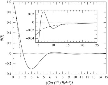
The decay of the variation in surfactant concentration resembles a damped oscillation, as shown in figure 3, but the amplitude of the variation becomes zero only three times and decays monotonically at late times. Determined numerically, the three roots
 $\tilde{t}_{i}$
of
 $\unicode[STIX]{x1D703}(\tilde{t})$
are
 $((2\unicode[STIX]{x03C0})^{4/3}/\mathit{Re}^{1/3})\tilde{t}_{i}=1.6452$
,
 $5.7437$
and
 $8.3765$
. Oscillations occur due to the inertia of the fluid that is set in motion by the surface stress distribution. Initially, regions with high surfactant concentration (lower surface tension) expand, while those with low concentration (higher tension) contract. When the surfactant distribution becomes uniform, first at
 $\tilde{t}_{1}$
, the fluid continues to expand/contract the surfactant distribution, which now creates regions of locally low/high concentration. The surface stresses then reverse the upper layer of the flow, and the surfactant distribution decays again. The surfactant concentration overshoots the equilibrium two more times before gradually decaying to uniformity. The finite number of oscillations distinguishes this system from a typical damped oscillator.
The decay over time of the amplitude of a sinusoidal surfactant concentration distribution at high
 $\mathit{Re}$
(3.23). The early time behaviour (3.26) is shown with a dash-dotted line. The inset emphasizes the finite number of roots and the absence of sustained oscillation, with the late-time monotonic decay (3.24) shown as a dashed line.

Using
 $\exp (z^{2})\text{erfc}(z)\sim (1/z\sqrt{\unicode[STIX]{x03C0}})(1-1/2z^{2})$
for large
 $z$
, obtained from the first two terms of the asymptotic expansion of
 $\text{erfc}$
(Olver et al.
Reference Olver, Lozier, Boisvert and Clark2010, equation (7.12.1); DLMF 2015), we find that at late times, deviations in surfactant concentration decay monotonically according to the power law
 $$\begin{eqnarray}\unicode[STIX]{x1D703}(\tilde{t})\sim -\frac{1}{2\sqrt{\unicode[STIX]{x03C0}}}\left(\frac{(2\unicode[STIX]{x03C0})^{4/3}}{\mathit{Re}^{1/3}}\tilde{t}\right)^{-3/2}.\end{eqnarray}$$
This result is shown as the dashed line in the inset of figure 3. Two terms in the approximation are required because
 $1/b_{0}+1/b_{+}+1/b_{-}=0$
, which makes the contribution of the first term vanish in the sum in equation (3.23).
The factor on
 $\tilde{t}$
in the solution for the surfactant decay, equation (3.23), shows that in the large
 $\mathit{Re}$
limit, the decay time scale is not the advective time scale
 $t^{\ast }=\unicode[STIX]{x1D706}/u^{\ast }$
. Instead, the surfactant decay time scale
 $t_{\unicode[STIX]{x1D6E4}}^{\ast }$
is the cube root of the product of the viscous time scale
 $\unicode[STIX]{x1D70C}\unicode[STIX]{x1D706}^{2}/\unicode[STIX]{x1D707}$
and the square of the advective time scale
 $t^{\ast }=\unicode[STIX]{x1D706}/u^{\ast }$
:
 $$\begin{eqnarray}t_{\unicode[STIX]{x1D6E4}}^{\ast }=t^{\ast }\mathit{Re}^{1/3}=\left(\frac{\unicode[STIX]{x1D70C}\unicode[STIX]{x1D706}^{4}\unicode[STIX]{x1D707}}{\unicode[STIX]{x1D6FC}^{2}\bar{\unicode[STIX]{x1D6E4}}^{2}}\right)^{1/3}=\left(t^{\ast 2}\frac{\unicode[STIX]{x1D70C}\unicode[STIX]{x1D706}^{2}}{\unicode[STIX]{x1D707}}\right)^{1/3}.\end{eqnarray}$$
One may still interpret this as an advective time scale with characteristic velocity
 $u^{\ast }/\mathit{Re}^{1/3}$
instead of
 $u^{\ast }$
.
The surfactant decay time scale also follows from a simple scaling argument. From the surfactant transport equation (3.1a
), we have
 $\unicode[STIX]{x2202}\tilde{\unicode[STIX]{x1D6E4}}/\unicode[STIX]{x2202}\tilde{t}\sim \unicode[STIX]{x2202}\tilde{u} _{s}/\unicode[STIX]{x2202}\tilde{x}\sim \tilde{u} _{s}$
, and the surface stress boundary condition (2.8) provides
 $\unicode[STIX]{x2202}\tilde{u} /\unicode[STIX]{x2202}{\tilde{y}}\sim \unicode[STIX]{x2202}\tilde{\unicode[STIX]{x1D6E4}}/\unicode[STIX]{x2202}\tilde{x}\sim \tilde{\unicode[STIX]{x1D6E4}}$
for
 ${\tilde{y}}\rightarrow 0^{+}$
. Making the approximation that
 $\unicode[STIX]{x2202}\tilde{u} /\unicode[STIX]{x2202}{\tilde{y}}\sim \tilde{u} _{s}/\tilde{\unicode[STIX]{x1D6FF}}$
, where
 $\tilde{\unicode[STIX]{x1D6FF}}\ll 1$
is a boundary layer thickness that grows over time as
 $\tilde{\unicode[STIX]{x1D6FF}}\sim (\tilde{t}/\mathit{Re})^{1/2}$
(this follows from the momentum equation (3.1b
) and
 $\mathit{Re}\,\unicode[STIX]{x2202}\tilde{u} /\unicode[STIX]{x2202}\tilde{t}\sim \unicode[STIX]{x2202}^{2}\tilde{u} /\unicode[STIX]{x2202}{\tilde{y}}^{2}$
), we obtain
 $\tilde{u} _{s}\sim \tilde{\unicode[STIX]{x1D6E4}}\tilde{\unicode[STIX]{x1D6FF}}$
. It follows that
 $\unicode[STIX]{x2202}\tilde{\unicode[STIX]{x1D6E4}}/\unicode[STIX]{x2202}\tilde{t}\sim (\tilde{t}/\mathit{Re})^{1/2}\tilde{\unicode[STIX]{x1D6E4}}$
, and scaling time by
 $\mathit{Re}^{-1/3}$
eliminates dependence on
 $\mathit{Re}$
. This result also indicates that at early times
 $\log \tilde{\unicode[STIX]{x1D6E4}}\sim \tilde{t}^{3/2}/\mathit{Re}^{1/2}$
, consistent with a series expansion of equation (3.23) about
 $\tilde{t}=0$
, which yields
 $$\begin{eqnarray}\unicode[STIX]{x1D703}(\tilde{t})=1-\frac{4}{3\sqrt{\unicode[STIX]{x03C0}}}\left(\frac{(2\unicode[STIX]{x03C0})^{4/3}}{\mathit{Re}^{1/3}}\tilde{t}\right)^{3/2}\end{eqnarray}$$
to leading order in
 $\tilde{t}$
.
3.2 Stokes flow limit
In the Stokes flow limit, i.e.
 $\mathit{Re}\rightarrow 0$
, of (2.10), the subsurface flow decays exponentially without oscillation (see also Masoud & Shelley Reference Masoud and Shelley2014). In this limit, the Laplace-domain solution for the surfactant evolution simplifies to
 $$\begin{eqnarray}\breve{\unicode[STIX]{x1D6E4}}(k,s)=\frac{1}{s+\unicode[STIX]{x03C0}}\hat{\unicode[STIX]{x1D6E4}}_{0}(k),\end{eqnarray}$$
and inversion provides
 $$\begin{eqnarray}\hat{\unicode[STIX]{x1D6E4}}(k,\tilde{t})=\exp (-\unicode[STIX]{x03C0}\tilde{t})\hat{\unicode[STIX]{x1D6E4}}_{0}(k).\end{eqnarray}$$
Furthermore, we obtain
 $$\begin{eqnarray}\displaystyle & \displaystyle \breve{p}(k,{\tilde{y}},s)=\breve{p}_{0}(k,s)\,\exp (-|k|{\tilde{y}}), & \displaystyle\end{eqnarray}$$
 $$\begin{eqnarray}\displaystyle & \displaystyle \breve{u}(k,{\tilde{y}},s)=-\frac{\text{i}}{2k}\breve{p}_{0}(k,s)\,\exp (-|k|{\tilde{y}})\,(|k|{\tilde{y}}-1), & \displaystyle\end{eqnarray}$$
 $$\begin{eqnarray}\displaystyle & \displaystyle \breve{v}(k,{\tilde{y}},s)={\textstyle \frac{1}{2}}\breve{p}_{0}(k,s)\,{\tilde{y}}\exp (-|k|{\tilde{y}}), & \displaystyle\end{eqnarray}$$
 $\tilde{\unicode[STIX]{x1D6E4}}_{0}(\tilde{x})=\sin (2\unicode[STIX]{x03C0}\tilde{x})$
follows as
 $$\begin{eqnarray}\displaystyle & \displaystyle \tilde{\unicode[STIX]{x1D6E4}}(\tilde{x},\tilde{t})=\sin (2\unicode[STIX]{x03C0}\tilde{x})\exp (-\unicode[STIX]{x03C0}\tilde{t}), & \displaystyle\end{eqnarray}$$
 $$\begin{eqnarray}\displaystyle & \displaystyle \tilde{u} (\tilde{x},{\tilde{y}},\tilde{t})=-{\textstyle \frac{1}{2}}\cos (2\unicode[STIX]{x03C0}\tilde{x})(1-2\unicode[STIX]{x03C0}{\tilde{y}})\exp (-2\unicode[STIX]{x03C0}{\tilde{y}})\exp (-\unicode[STIX]{x03C0}\tilde{t}), & \displaystyle\end{eqnarray}$$
 $$\begin{eqnarray}\displaystyle & \displaystyle \tilde{v}(\tilde{x},{\tilde{y}},\tilde{t})=-{\textstyle \frac{1}{2}}\sin (2\unicode[STIX]{x03C0}\tilde{x})(2\unicode[STIX]{x03C0}{\tilde{y}})\exp (-2\unicode[STIX]{x03C0}{\tilde{y}})\exp (-\unicode[STIX]{x03C0}\tilde{t}), & \displaystyle\end{eqnarray}$$
 $$\begin{eqnarray}\displaystyle & \displaystyle \tilde{p}_{0}(\tilde{x},\tilde{t})=-2\unicode[STIX]{x03C0}\sin (2\unicode[STIX]{x03C0}\tilde{x})\exp (-\unicode[STIX]{x03C0}\tilde{t}). & \displaystyle\end{eqnarray}$$
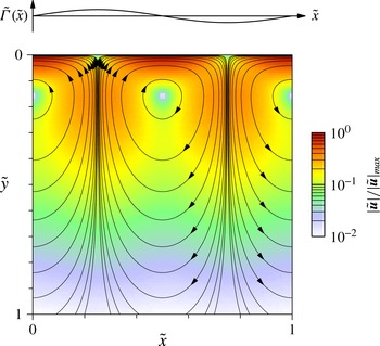
Stokes flow solution for the initial surfactant distribution
 $\tilde{\unicode[STIX]{x1D6E4}}_{0}(\tilde{x})=\sin (2\unicode[STIX]{x03C0}\tilde{x})$
in the subdomain
 $[0,1]\times [0,1]$
of the semi-infinite domain. The structure of the flow remains constant as it decays exponentially.

3.3 Developing flow under a steady surfactant distribution
To highlight how the time scale of the coupled transient problem differs from the advective and viscous time scales, we consider briefly a simpler problem: the response of the fluid to a sudden and sustained change in surfactant distribution. In contrast, the surfactant distribution in the coupled problem is initially changed and then allowed to evolve over time. Specifically, we consider the response of a motionless fluid to
 $\tilde{\unicode[STIX]{x1D6E4}}(\tilde{x},\tilde{t})=\sin (2\unicode[STIX]{x03C0}\tilde{x})H(\tilde{t})$
where
 $H(\cdot )$
is the Heaviside step function. For this condition, we have
 $$\begin{eqnarray}\hat{\unicode[STIX]{x1D6E4}}(k,\tilde{t})=-\text{i}\unicode[STIX]{x03C0}\,\text{sgn}(k)\,\unicode[STIX]{x1D6FF}(|k|-2\unicode[STIX]{x03C0})\,H(\tilde{t}),\quad \breve{\unicode[STIX]{x1D6E4}}(k,s)=-\frac{\text{i}\unicode[STIX]{x03C0}}{s}\,\text{sgn}(k)\,\unicode[STIX]{x1D6FF}(|k|-2\unicode[STIX]{x03C0}).\end{eqnarray}$$
Using (3.9a ) and (3.10), the Laplace-domain solution for the surface speed is
 $$\begin{eqnarray}\breve{u}(k,0,s)=-\frac{4\unicode[STIX]{x03C0}^{3}}{\mathit{Re}\,s^{2}}\left(\sqrt{1+\frac{\mathit{ Re }\,s}{4\unicode[STIX]{x03C0}^{2}}}-1\right)\unicode[STIX]{x1D6FF}(|k|-2\unicode[STIX]{x03C0}),\end{eqnarray}$$
and upon inverting the Laplace (Erdélyi et al. Reference Erdélyi, Magnus, Oberhettinger and Tricomi1954) and Fourier transforms, we obtain the time-domain solution
 $$\begin{eqnarray}\displaystyle \tilde{u} (\tilde{x},0,\tilde{t})=-\cos (2\unicode[STIX]{x03C0}\tilde{x})\left[\frac{1}{2}\,\text{erf}\left(\sqrt{\tilde{t}^{\prime }}\right)-\tilde{t}^{\prime }\,\text{erfc}\left(\sqrt{\tilde{t}^{\prime }}\right)+\sqrt{\frac{\tilde{t}^{\prime }}{\unicode[STIX]{x03C0}}}\exp (-\tilde{t}^{\prime })\right], & & \displaystyle\end{eqnarray}$$
where
 $\tilde{t}^{\prime }=4\unicode[STIX]{x03C0}^{2}\tilde{t}/\mathit{Re}$
. This solution is a monotonic rise in time to a steady state. The effect of
 $\mathit{Re}$
here is a rescaling of time. The time scale for the development of a flow under a steady stress distribution is the viscous time scale
 $\unicode[STIX]{x1D70C}\unicode[STIX]{x1D706}^{2}/\unicode[STIX]{x1D707}$
in contrast to the advective time scale
 $t^{\ast }$
of the coupled problem in the Stokes flow limit and
 $t_{\unicode[STIX]{x1D6E4}}^{\ast }$
in the high
 $\mathit{Re}$
limit.
4 Numerical results
We now investigate numerically the situations not addressed by the analytical cases, specifically large-amplitude variation in
 $\unicode[STIX]{x1D6E4}$
and behaviour at intermediate
 $\mathit{Re}$
. We use a semi-implicit spectral finite difference method in the vorticity–streamfunction form (for details see appendix A). The approach is similar to that followed for the analytical solution but retains the nonlinear terms. A Fourier transform is used in the
 $x$
direction, and second-order central finite differences are used in the
 $y$
direction. The height of the simulation domain is finite, and the boundary condition for the vorticity on the no-slip boundary is applied using Thom’s formula (Thom Reference Thom1933). Integration in time is performed with the second-order Adams–Bashforth method after an initial explicit Euler time step. The resolution of the simulations is 64 points in the
 $x$
direction and 257 in
 $y$
for a domain with a height that is double its width. This aspect ratio is judged to be sufficiently high to approximate a semi-infinite domain because in the worst case of Stokes flow, the flow speed for the fundamental mode in a semi-infinite domain decays by four orders of magnitude within this depth. The spatial resolution in
 $y$
is twice the resolution in
 $x$
, chosen to resolve the flow near the surface. Unless specified otherwise, the initial condition is
 $\tilde{\unicode[STIX]{x1D6E4}}_{0}(\tilde{x})=\sin (2\unicode[STIX]{x03C0}\tilde{x})$
.
4.1 Steady surfactant distribution
As a benchmark, we examine first the transient solution for the flow developing from rest under a steady surfactant distribution, i.e.
 $\unicode[STIX]{x1D6E4}(x,t)=\unicode[STIX]{x1D6E4}_{0}(x)~\text{for}~t>0$
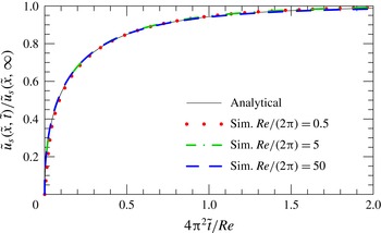
. The computed surface speed as a function of time, shown in figure 5 for
 $\mathit{Re}/(2\unicode[STIX]{x03C0})=0.5$
, 5, and 50 with
 $\unicode[STIX]{x1D700}=0.1$
, agrees well with the analytical solution, equation (3.33). Though not shown, deviation from the analytical solution begins with
 $\unicode[STIX]{x1D700}\mathit{Re}/(2\unicode[STIX]{x03C0})\approx 10$
due to the nonlinear term in (2.10) that was neglected in the derivation of the analytical solution.
Comparison of the analytical solution for the development of the surface flow due to a constant sinusoidal surfactant distribution, equation (3.33), and simulations with
 $\unicode[STIX]{x1D700}=0.1$
and
 $\mathit{Re}/(2\unicode[STIX]{x03C0})=0.5$
, 5 and 50. The flow evolves in the same way for all
 $\tilde{x}$
.

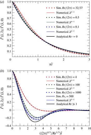
Numerical and analytical solutions for the decay of small variations in the surfactant concentration with (a)
 $\mathit{Re}/(2\unicode[STIX]{x03C0})\leqslant 32/27$
and (b)
 $\mathit{Re}/(2\unicode[STIX]{x03C0})>32/27$
. The dotted curves show the simulation results (with
 $\unicode[STIX]{x1D700}=0.01$
), the coloured solid lines show numerical inversion of the Laplace domain solution (3.13), and the solid black lines show the analytical solutions ((3.28) for
 $\mathit{Re}\rightarrow 0$
and (3.23) for
 $\mathit{Re}\gg 1$
). The curves with large dots were computed with sufficiently high
 $\mathit{Pe}_{s}$
that diffusion is negligible (
 $\mathit{Pe}_{s}=1000$
in (a) and in (b)
 $\mathit{Pe}_{s}=1587$
, 4641 and 10 000 for
 $\mathit{Re}/(2\unicode[STIX]{x03C0})=4$
, 100 and 1000, respectively), while the curve with smaller dots in (b) shows the computed result for
 $\mathit{Re}/(2\unicode[STIX]{x03C0})=1000$
with
 $\mathit{Pe}_{s}=500$
.

4.2 Small
$\unicode[STIX]{x1D700}$

Simulations of the full transient problem with decaying small-amplitude (
 $\unicode[STIX]{x1D700}\rightarrow 0$
) variations in the surfactant concentration and high
 $\mathit{Pe}_{s}$
are shown in figure 6. In the limits of small and large
 $\mathit{Re}$
, the numerical results approach the corresponding analytical solutions. For intermediate
 $\mathit{Re}$
, the simulation results were compared with numerical inversion of the Laplace-domain solution (3.14). Since the simulations include the surfactant diffusion term, a sufficiently large value of
 $\mathit{Pe}_{s}$
is required to keep diffusion negligible. The choice of
 $\mathit{Pe}_{s}$
must ensure that the diffusion time scale is significantly longer than the surfactant decay time scale, which is not necessarily the advection time scale used to define
 $\mathit{Pe}_{s}$
. In the limit of low
 $\mathit{Re}$
, we require
 $$\begin{eqnarray}\frac{\unicode[STIX]{x1D706}^{2}}{D_{s}}\gg \frac{t^{\ast }}{\unicode[STIX]{x03C0}}\Rightarrow \mathit{Pe}_{s}\gg 1,\end{eqnarray}$$
whereas in the high
 $\mathit{Re}$
limit the requirement is
 $$\begin{eqnarray}\frac{\unicode[STIX]{x1D706}^{2}}{D_{s}}\gg \frac{\mathit{Re}^{1/3}t^{\ast }}{(2\unicode[STIX]{x03C0})^{4/3}}\Rightarrow \frac{(2\unicode[STIX]{x03C0})^{4/3}}{\mathit{Re}^{1/3}}\mathit{Pe}_{s}\gg 1,\end{eqnarray}$$
which follows from (3.25). While a fixed high
 $\mathit{Pe}_{s}$
is suitable at low
 $\mathit{Re}$
, in which case the surfactant decay time scale is the advection time scale,
 $\mathit{Pe}_{s}$
must be scaled in proportion to
 $\mathit{Re}^{1/3}$
for high
 $\mathit{Re}$
. The simulations in figure 6(a) all had
 $\mathit{Pe}_{s}=1000$
, while those in figure 6(b) were performed with
 $\mathit{Pe}_{s}=1587$
, 4641 and 10 000 for
 $\mathit{Re}/(2\unicode[STIX]{x03C0})=4$
, 100 and 1000, respectively. For these values,
 $(\mathit{Re}/(2\unicode[STIX]{x03C0}))^{-1/3}\mathit{Pe}_{s}=1000$
. Good agreement in all cases with the Laplace-domain solution for infinite
 $\mathit{Pe}_{s}$
indicates that these choices of
 $\mathit{Pe}_{s}$
are satisfactory to suppress the effects of diffusion. For comparison, a simulation with
 $\mathit{Pe}_{s}=500$
and
 $\mathit{Re}/(2\unicode[STIX]{x03C0})=1000$
is also shown in figure 6. At this lower
 $\mathit{Pe}_{s}$
, agreement with the high
 $\mathit{Pe}_{s}$
solution is still reasonable. Though not shown in figure 6, the surfactant distribution continues to decay faster as
 $\mathit{Pe}_{s}$
is decreased further. With
 $\mathit{Pe}_{s}=10$
, the minimum becomes
 $-0.01$
at
 $[(2\unicode[STIX]{x03C0})^{4/3}/\mathit{Re}^{1/3}]\tilde{t}\approx 1.5$
.
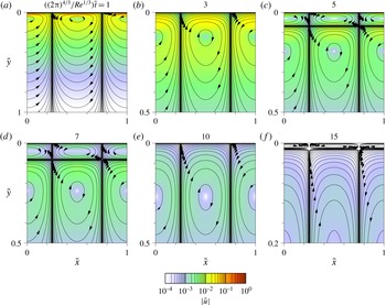
The evolution of the flow structure at
 $\mathit{Re}/(2\unicode[STIX]{x03C0})=100$
and
 $\unicode[STIX]{x1D700}=0.01$
is illustrated in figure 7. As mentioned earlier, the oscillations in the surfactant concentration occur due to the inertia of the flow when the surfactant concentration first becomes uniform. During the initial decay in the amplitude of the surfactant variation, its first zero crossing, and subsequent growth, the flow structure consists of a row of counter-rotating vortices that penetrate deeper into the fluid layer over time. A second layer of vortices forms above the initial layer when the first peak in amplitude (of the opposite sign to the initial condition) is reached. The change in sign of the surface stress therefore reverses the motion of the surfactant and creates this new layer of vortices rather than stopping and reversing the initial vortex layer. The flow structure alternates between having one and two layers of vortices until the third and final peak in amplitude. The flow and surfactant concentration variation then decay monotonically to zero with two rows of vortices present. The development of the flow for
 $\mathit{Re}/(2\unicode[STIX]{x03C0})=100$
is representative of the structure seen in the oscillatory decay regime (
 $\mathit{Re}/(2\unicode[STIX]{x03C0})>32/27$
). With increasing
 $\mathit{Re}$
, however, the vortices are compressed vertically.
Evolution of the flow structure at
 $\mathit{Re}/(2\unicode[STIX]{x03C0})=100$
and
 $\unicode[STIX]{x1D700}=0.01$
in the upper half (a), quarter (b–e), and fifth (f) of the simulated domain. The colour indicates the flow speed, and a logarithmic colour scale is used for convenience. Time proceeds from (a) to (f). Different ranges of the vertical axes in (a) and (f) are used to emphasize the structure of the flow.

4.3 Initial conditions with multiple modes
Due to the linearity of the governing equations in the limit of small
 $\unicode[STIX]{x1D700}$
, the solutions for arbitrary periodic initial surfactant distributions can be constructed by superposition of the solutions for single modes. Expanding
 $\tilde{\unicode[STIX]{x1D6E4}}_{0}(\tilde{x})$
for
 $\tilde{x}\in [0,1]$
in a Fourier series as
 $\sum _{n=1}^{\infty }a_{n}\sin (2\unicode[STIX]{x03C0}n\tilde{x}+\unicode[STIX]{x1D719}_{n})$
, we see that the solution will consist of the single-mode solutions for wavelengths
 $\unicode[STIX]{x1D706}_{n}=\unicode[STIX]{x1D706}_{1}/n$
where
 $\unicode[STIX]{x1D706}_{1}$
is the wavelength of the fundamental mode. These modes have corresponding Reynolds numbers
 $\mathit{Re}_{n}=\mathit{Re}_{1}/n$
and time scales
 $t_{n}^{\ast }=t_{1}^{\ast }/n$
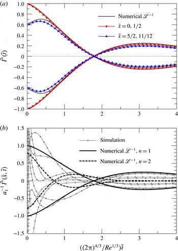
. The fundamental mode decays slowest, as shown in figure 8 for (a) an initial distribution that has two modes and (b) one that is random. For the simulation with two modes,
 $\mathit{Pe}_{s}$
was chosen as 20 800 to satisfy equation (4.2) for the
 $n=3$
mode; for the random distribution,
 $\mathit{Pe}_{s}=10\,000$
for the fundamental mode. The evolution of the random distribution shows that when the fundamental mode reaches its first zero, the third and higher modes are effectively negligible because the solution at this time is bounded by the amplitude of the second mode.
The decay of initial surfactant distributions with multiple modes. The time axis is scaled using the Reynolds number for the fundamental mode,
 $\mathit{Re}_{1}$
, with
 $\mathit{Re}_{1}/(2\unicode[STIX]{x03C0})=1000$
and
 $\unicode[STIX]{x1D700}=0.01$
for both cases. In (a), the initial condition is
 $\tilde{\unicode[STIX]{x1D6E4}}_{0}(\tilde{x})=\cos (2\unicode[STIX]{x03C0}\tilde{x})+(1/4)\sin (6\unicode[STIX]{x03C0}\tilde{x})$
. The numerical solutions (coloured lines with symbols) are compared with numerical inversion of the Laplace-domain solution (solid black lines) at
 $\tilde{x}=0$
,
 $5/12$
,
 $1/2$
and
 $11/12$
. In (b),
 $\tilde{\unicode[STIX]{x1D6E4}}_{0}$
is a random value from
 $[-1,1]$
at each point in the simulated domain. The concentrations are shown at positions
 $\tilde{x}$
that are multiples of
 $1/8$
(grey lines with dots), and they are scaled by the magnitude
 $a_{1}$
of the fundamental mode in the initial condition. The black lines show the decay of the first (
 $n=1$
, solid) and second (
 $n=2$
, dashed) modes in the initial distribution obtained by numerical inversion of the Laplace-domain solution and evaluated at the positions of maximum amplitude for each mode.

4.4 Finite
$\unicode[STIX]{x1D700}$

For small
 $\unicode[STIX]{x1D700}$
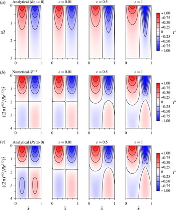
, the portions of the surface with positive and negative deviation from the mean surfactant concentration evolve symmetrically, and this case is described by the analytical and Laplace-domain solutions. The simulations in figure 9 show the asymmetry in the evolution of the surfactant as
 $\unicode[STIX]{x1D700}$
increases to one, which is its upper bound since negative concentrations are inadmissible. While the results for
 $\unicode[STIX]{x1D700}=0.01$
match the
 $\unicode[STIX]{x1D700}\rightarrow 0$
solutions, the region with positive
 $\tilde{\unicode[STIX]{x1D6E4}}$
initially widens and decays faster for higher
 $\unicode[STIX]{x1D700}$
with low
 $\mathit{Re}$
(figure 9
a), the region with negative
 $\tilde{\unicode[STIX]{x1D6E4}}$
narrows, and the concentration profile sharpens around the minimum. These effects are due to the nonlinear term in (2.9), which accelerates the decrease of
 $\tilde{\unicode[STIX]{x1D6E4}}$
near its maximum, makes
 $\unicode[STIX]{x2202}\tilde{\unicode[STIX]{x1D6E4}}/\unicode[STIX]{x2202}\tilde{t}$
non-zero where initially
 $\tilde{\unicode[STIX]{x1D6E4}}\approx 0$
, and decreases
 $\unicode[STIX]{x2202}\tilde{\unicode[STIX]{x1D6E4}}/\unicode[STIX]{x2202}\tilde{t}$
near the minimum
 $\tilde{\unicode[STIX]{x1D6E4}}$
. In fact, as will be described in greater detail for higher
 $\mathit{Re}$
, the convective term vanishes at the minimum
 $\tilde{\unicode[STIX]{x1D6E4}}$
as
 $\unicode[STIX]{x1D700}\rightarrow 1$
leaving only diffusion to drive changes in concentration there.
Evolution of the surfactant concentration in the limit
 $\unicode[STIX]{x1D700}\rightarrow 0$
(analytical solutions or numerical inversion of Laplace-domain solution) and numerical solutions for finite-amplitude variation in concentration (
 $\unicode[STIX]{x1D700}=0.01$
, 0.5 and 1) at (a)
 $\mathit{Re}/(2\unicode[STIX]{x03C0})=0.1$
, (b) 100 and (c) 1000.

At the higher
 $\mathit{Re}$
, for which oscillations occur (figure 9
b,c), the effects of increasing
 $\unicode[STIX]{x1D700}$
are more complex because of the nonlinear terms in both the surfactant evolution and fluid flow. At early times (
 $[(2\unicode[STIX]{x03C0})^{4/3}/\mathit{Re}^{1/3}]\tilde{t}<1$
), the behaviour is similar to that with lower
 $\mathit{Re}$
. Unlike at lower
 $\mathit{Re}$
, the concentration at the minimum then begins to increase faster, and for
 $\unicode[STIX]{x1D700}=1$
, the growth rate exceeds that in the immediately adjacent regions, and a local maximum and two adjacent minima form in the surfactant concentration. This local maximum is more pronounced and occurs earlier at the highest
 $\mathit{Re}$
. From
 $[(2\unicode[STIX]{x03C0})^{4/3}/\mathit{Re}^{1/3}]\tilde{t}\approx 1.5$
to 2, a temporary doubling in the spatial frequency of the concentration profile is evident.
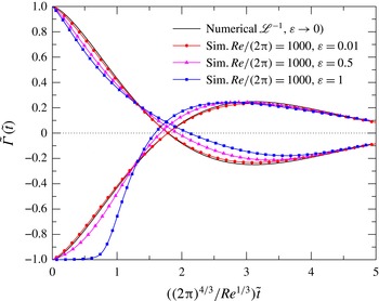
The asymmetry in the evolution of the surfactant concentrations at the locations of the initial minimum and maximum is emphasized in figure 10. The most significant change in the dynamics with increasing
 $\unicode[STIX]{x1D700}$
is the emergence of a delay in the growth of the concentration from
 $\tilde{\unicode[STIX]{x1D6E4}}=-1$
. In figure 9, this was seen as a narrowing of the region with negative
 $\tilde{\unicode[STIX]{x1D6E4}}$
. For
 $\unicode[STIX]{x1D700}$
approaching sufficiently close to one, the advective terms in the surfactant dynamics become negligible for any
 $\mathit{Pe}_{s}$
, leaving only diffusion to drive changes in
 $\tilde{\unicode[STIX]{x1D6E4}}$
at early times. The diffusive flux that determines the duration of the initial delay depends on the initial concentration profile and the developing flow, which sharpens the profile, increasing the flux. The dominance of the diffusive term persists until
 $\tilde{\unicode[STIX]{x1D6E4}}$
increases sufficiently that the advective terms take over. Due to the effect of diffusion on the initial delay, the surfactant evolution for high
 $\unicode[STIX]{x1D700}$
is expected to depend on
 $\mathit{Pe}_{s}$
.
Asymmetry in the decay of the surfactant concentration from its maximum and minimum values at
 $\mathit{Re}/(2\unicode[STIX]{x03C0})=1000$
,
 $\mathit{Pe}_{s}=10\,000$
, and several
 $\unicode[STIX]{x1D700}$
. The solid black line shows the numerical inversion of the Laplace-domain solution for the limit of
 $\unicode[STIX]{x1D700}\rightarrow 0$
, equation (3.14).

4.5 Parameters for physical systems
Where do typical physical systems lie in the dimensionless parameter space and how would they behave? Consider an aqueous surfactant solution with a clean surface tension
 $\unicode[STIX]{x1D6FE}_{0}$
of
 $72~\text{mN}~\text{m}^{-1}$
and 10 % variation in tension around a mean of
 $50~\text{mN}~\text{m}^{-1}$
. Using
 $\unicode[STIX]{x1D70C}=1000~\text{kg}~\text{m}^{-3}$
and
 $\unicode[STIX]{x1D707}=1~\text{mPa}~\text{s}$
, we obtain
 $\mathit{Re}=2.2\times 10^{4}$
for a millimetre-scale variation in surface tension. The advective time scale is
 $45~\unicode[STIX]{x03BC}\text{s}$
. Assuming a diffusivity of the order of
 $10^{-9}~\text{m}^{2}~\text{s}^{-1}$
, which is typical of small solute molecules, the diffusive time scale is
 $\unicode[STIX]{x1D706}^{2}/D_{s}=10^{3}~\text{s}$
and
 $\mathit{Pe}_{s}=2.2\times 10^{7}$
. This system is clearly in the high
 $\mathit{Re}$
limit and the surfactant decay time scale is
 $1.3~\text{ms}$
, much shorter than the diffusive time scale. For centimetre-scale variation,
 $\mathit{Re}=2.2\times 10^{5}$
, the advective time scale is
 $0.45~\text{ms}$
, the diffusive time scale is
 $10^{5}~\text{s}$
,
 $\mathit{Pe}_{s}=2.2\times 10^{8}$
and the surfactant decay time scale is
 $27~\text{ms}$
. For both these sample sets of parameters, the surfactant decay time scales are significantly shorter than the diffusion time scales, satisfying the key assumption in the modelling that
 $\mathit{Pe}_{s}$
is large and diffusion can be neglected. The diffusivities of larger solute molecules can be up to several orders of magnitude lower, such as
 $10^{-10}~\text{m}^{2}~\text{s}^{-1}$
for sodium dodecyl sulphate, and values of
 $\mathit{Pe}_{s}$
for such solutes would be correspondingly higher. Considering that Schmidt numbers
 $\mathit{Sc}_{s}=\unicode[STIX]{x1D707}/(\unicode[STIX]{x1D70C}D_{s})=\mathit{Pe}_{s}/\mathit{Re}$
for aqueous systems are typically
 $O(1000)$
, the assumption of high
 $\mathit{Pe}_{s}$
is reasonable for the oscillatory surfactant decay regime in which
 $\mathit{Re}$
exceeds one. The effects of diffusion need to be included for lower
 $\mathit{Re}$
, however, unless the system has a higher
 $\mathit{Sc}_{s}$
. The high
 $\mathit{Re}$
of the sample systems, which exceed those considered in this paper for
 $\unicode[STIX]{x1D700}>0$
, motivate further study of nonlinear phenomena at high
 $\mathit{Re}$
and finite
 $\unicode[STIX]{x1D700}$
, in particular the limit
 $\unicode[STIX]{x1D700}\rightarrow 1$
.
5 Conclusions
We have presented analytical solutions for the decay of small-amplitude variations in the concentration of an insoluble surfactant on an initially motionless and infinitely deep layer of a Newtonian liquid. Surfactant diffusion was neglected in the analytical solutions. While the surfactant decays monotonically (and exponentially) in the Stokes flow limit, for unsteady Stokes flow at higher
 $\mathit{Re}$
, the amplitude of the surfactant concentration distribution oscillates, changing sign three times before decaying monotonically at late times as
 $t^{-3/2}$
. A unique feature of the dynamics of this system is this finite number of oscillations, which distinguishes it from a typical damped simple harmonic oscillator. During the oscillations, the structure of the flow below the surface alternates between one and two layers of counter-rotating vortices. The origin of the oscillations is the inertia of the flow induced by the initial surface Marangoni stress distribution, which drives the surfactant concentration beyond a uniform equilibrium distribution. The analytical solution for the surfactant concentration in the limit of large
 $\mathit{Re}$
reveals that the time scale for surfactant decay (and oscillation) is the cube root of the product of the viscous time scale and the square of the advective time scale. In contrast, at low
 $\mathit{Re}$
the decay time scale is simply the advective time scale.
We used a hybrid spectral–finite difference method to examine the nonlinear problem of finite-amplitude (
 $\unicode[STIX]{x1D700}$
) variations in surfactant concentration in the limit of high surface Péclet number. Increases in
 $\unicode[STIX]{x1D700}$
create an asymmetry in the evolution of regions with above- and below-average surfactant concentration. The portion of the surface with a positive deviation from the mean initially widens and decays faster than it would for lower
 $\unicode[STIX]{x1D700}$
, while growth in the portion with a negative deviation is delayed. In the limit
 $\unicode[STIX]{x1D700}\rightarrow 1$
, the delay is significant and is caused by diffusion of the surfactant dominating over advection at early times in the vicinity of the minimum (near zero) concentration. At high
 $\mathit{Re}$
, the rapid growth after the delay creates an additional local maximum and two adjacent minima in the concentration profile, which contribute higher-frequency components to the surfactant distribution than the initial fundamental frequency.
Since typical aqueous systems would have higher
 $\mathit{Re}$
than those we considered at present (see § 4.5), nonlinear phenomena in the behaviour of surfactants at higher
 $\mathit{Re}$
with large-amplitude variations in concentration deserve further attention (i.e. the limit of
 $\unicode[STIX]{x1D700}\rightarrow 1$
and
 $\mathit{Re}\gg 1$
). A wide variety of additional physical and chemical phenomena could also be included in the model to examine their effects on the evolution and oscillation of surfactant distributions. Possibilities include soluble surfactants, confinement (i.e. finite height of the fluid layer), a deforming surface, two viscous fluids, reactions and surfactant adsorption/desorption at the interface and the evolution of two-dimensional surfactant patterns on a three-dimensional fluid domain. In physiological systems, which can be significantly more viscous than higher purity aqueous systems, the effects of non-Newtonian rheology, such as shear thinning, could also be considered. A better understanding of surfactant and flow dynamics on interfaces could be used to enhance heat and mass transfer and study the motion of individual organisms and inanimate particles on interfaces, as well as the collective motion of many such particles.
Acknowledgement
O.S. thanks the Natural Sciences and Engineering Research Council of Canada (NSERC) for a postdoctoral fellowship.
Appendix A. Numerical method
The transport equation for the surfactant concentration, including diffusion, on a non-deforming planar surface is:
 $$\begin{eqnarray}\frac{\unicode[STIX]{x2202}\unicode[STIX]{x1D6E4}}{\unicode[STIX]{x2202}t}+\unicode[STIX]{x1D735}_{s}\boldsymbol{\cdot }(\unicode[STIX]{x1D6E4}\boldsymbol{u}_{s})=D_{s}\unicode[STIX]{x1D6FB}_{s}^{2}\unicode[STIX]{x1D6E4},\end{eqnarray}$$
where
 $\boldsymbol{u}_{s}(\boldsymbol{x},t)=\boldsymbol{u}(\boldsymbol{x},y=0,t)$
,
 $\boldsymbol{x}$
is the position on the plane and
 $y$
is perpendicular to it and extends into the adjacent fluid. Since surfactant is transported only in one direction,
 $x$
, in the plane, the equation above reduces to
 $$\begin{eqnarray}\frac{\unicode[STIX]{x2202}\unicode[STIX]{x1D6E4}}{\unicode[STIX]{x2202}t}+\frac{\unicode[STIX]{x2202}}{\unicode[STIX]{x2202}x}(\unicode[STIX]{x1D6E4}u_{s})=D_{s}\frac{\unicode[STIX]{x2202}^{2}\unicode[STIX]{x1D6E4}}{\unicode[STIX]{x2202}x^{2}}.\end{eqnarray}$$
Taking the Fourier transform of both sides in
 $x$
we have
 $$\begin{eqnarray}\frac{\unicode[STIX]{x2202}\hat{\unicode[STIX]{x1D6E4}}}{\unicode[STIX]{x2202}t}+\text{i}k\widehat{u_{s}\unicode[STIX]{x1D6E4}}=-D_{s}k^{2}\hat{\unicode[STIX]{x1D6E4}},\end{eqnarray}$$
which can also be written as
 $$\begin{eqnarray}\frac{\unicode[STIX]{x2202}}{\unicode[STIX]{x2202}t}[\exp (D_{s}k^{2}t)\hat{\unicode[STIX]{x1D6E4}}]=-\text{exp}\,(D_{s}k^{2}t)\text{i}k\widehat{u_{s}\unicode[STIX]{x1D6E4}}.\end{eqnarray}$$
In the discrete form, the first time step uses the first-order Euler method:
 $$\begin{eqnarray}\hat{\unicode[STIX]{x1D6E4}}^{m+1}=\exp (-D_{s}k^{2}\unicode[STIX]{x0394}t)[\hat{\unicode[STIX]{x1D6E4}}^{m}-\text{i}k\unicode[STIX]{x0394}t\widehat{u_{s}\unicode[STIX]{x1D6E4}}^{m}].\end{eqnarray}$$
All subsequent time steps use the second-order Adams–Bashforth method:
 $$\begin{eqnarray}\hat{\unicode[STIX]{x1D6E4}}^{m+1}=\exp (-D_{s}k^{2}\unicode[STIX]{x0394}t)\left[\hat{\unicode[STIX]{x1D6E4}}^{m}-\frac{\text{i}k\unicode[STIX]{x0394}t}{2}(3\widehat{u_{s}\unicode[STIX]{x1D6E4}}^{m}-\exp (-D_{s}k^{2}\unicode[STIX]{x0394}t)\widehat{u_{s}\unicode[STIX]{x1D6E4}}^{m-1})\right].\end{eqnarray}$$
While analytical solutions were obtained for a semi-infinite two-dimensional system, a finite domain size (
 $W$
in
 $x$
and
 $H$
in
 $y$
) is used for the simulations. The Navier–Stokes equations for the fluid in the bulk can be written in the vorticity–streamfunction form as
 $$\begin{eqnarray}\displaystyle & \displaystyle \frac{\unicode[STIX]{x2202}\unicode[STIX]{x1D714}}{\unicode[STIX]{x2202}t}+\boldsymbol{u}\boldsymbol{\cdot }\unicode[STIX]{x1D735}\unicode[STIX]{x1D714}=\unicode[STIX]{x1D708}\unicode[STIX]{x1D6FB}^{2}\unicode[STIX]{x1D714}, & \displaystyle\end{eqnarray}$$
 $$\begin{eqnarray}\displaystyle & \displaystyle \unicode[STIX]{x1D6FB}^{2}\unicode[STIX]{x1D713}=\unicode[STIX]{x1D714}, & \displaystyle\end{eqnarray}$$
 $\unicode[STIX]{x1D708}=\unicode[STIX]{x1D707}/\unicode[STIX]{x1D70C}$
and
 $$\begin{eqnarray}u=\frac{\unicode[STIX]{x2202}\unicode[STIX]{x1D713}}{\unicode[STIX]{x2202}y},\quad v=-\frac{\unicode[STIX]{x2202}\unicode[STIX]{x1D713}}{\unicode[STIX]{x2202}x}.\end{eqnarray}$$
The boundary conditions are
 $$\begin{eqnarray}u(0,y)=u(W,y),\quad v(0,y)=v(W,y),\end{eqnarray}$$
 $$\begin{eqnarray}\unicode[STIX]{x1D707}\frac{\unicode[STIX]{x2202}u}{\unicode[STIX]{x2202}y}(x,0)=-\frac{\unicode[STIX]{x2202}\unicode[STIX]{x1D6FE}}{\unicode[STIX]{x2202}x}=\unicode[STIX]{x1D6FC}\frac{\unicode[STIX]{x2202}\unicode[STIX]{x1D6E4}}{\unicode[STIX]{x2202}x},\quad v(x,0)=0,\quad u(x,H)=v(x,H)=0.\end{eqnarray}$$
The domain is periodic in
 $x$
, has a Marangoni stress distribution at
 $y=0$
and a no-slip wall at
 $y=H$
. The boundary conditions for the vorticity and streamfunction are:
 $$\begin{eqnarray}\unicode[STIX]{x1D714}(x,0)=\frac{\unicode[STIX]{x2202}u}{\unicode[STIX]{x2202}y}(x,0)=\frac{\unicode[STIX]{x1D6FC}}{\unicode[STIX]{x1D707}}\frac{\unicode[STIX]{x2202}\unicode[STIX]{x1D6E4}}{\unicode[STIX]{x2202}x},\end{eqnarray}$$
 $$\begin{eqnarray}\unicode[STIX]{x1D714}(0,y)=\unicode[STIX]{x1D714}(W,y),\quad \frac{\unicode[STIX]{x2202}\unicode[STIX]{x1D714}}{\unicode[STIX]{x2202}x}(0,y)=\frac{\unicode[STIX]{x2202}\unicode[STIX]{x1D714}}{\unicode[STIX]{x2202}x}(W,y),\end{eqnarray}$$
 $$\begin{eqnarray}\unicode[STIX]{x1D713}(x,0)=0,\quad \unicode[STIX]{x1D713}(x,H)=0,\quad \frac{\unicode[STIX]{x2202}\unicode[STIX]{x1D713}}{\unicode[STIX]{x2202}y}(x,H)=0,\end{eqnarray}$$
 $$\begin{eqnarray}\unicode[STIX]{x1D713}(0,y)=\unicode[STIX]{x1D713}(W,y),\quad \frac{\unicode[STIX]{x2202}\unicode[STIX]{x1D713}}{\unicode[STIX]{x2202}x}(0,y)=\frac{\unicode[STIX]{x2202}\unicode[STIX]{x1D713}}{\unicode[STIX]{x2202}x}(W,y).\end{eqnarray}$$
Taking the Fourier transform in
 $x$
we have
 $$\begin{eqnarray}\displaystyle & \displaystyle \frac{\unicode[STIX]{x2202}\hat{\unicode[STIX]{x1D714}}}{\unicode[STIX]{x2202}t}+\widehat{\boldsymbol{u}\boldsymbol{\cdot }\unicode[STIX]{x1D735}\unicode[STIX]{x1D714}}=\unicode[STIX]{x1D708}\left(\frac{\unicode[STIX]{x2202}^{2}\hat{\unicode[STIX]{x1D714}}}{\unicode[STIX]{x2202}y^{2}}-k^{2}\hat{\unicode[STIX]{x1D714}}\right), & \displaystyle\end{eqnarray}$$
 $$\begin{eqnarray}\displaystyle & \displaystyle \frac{\unicode[STIX]{x2202}^{2}\hat{\unicode[STIX]{x1D713}}}{\unicode[STIX]{x2202}y^{2}}-k^{2}\hat{\unicode[STIX]{x1D713}}=\hat{\unicode[STIX]{x1D714}}, & \displaystyle\end{eqnarray}$$
 $$\begin{eqnarray}\displaystyle & \displaystyle \hat{\unicode[STIX]{x1D714}}(k,0)=\text{i}k\frac{\unicode[STIX]{x1D6FC}}{\unicode[STIX]{x1D707}}\hat{\unicode[STIX]{x1D6E4}}, & \displaystyle\end{eqnarray}$$
 $$\begin{eqnarray}\displaystyle \hat{\unicode[STIX]{x1D713}}(x,0)=0,\quad \hat{\unicode[STIX]{x1D713}}(x,H)=0, & & \displaystyle\end{eqnarray}$$
which can be written in discrete form as (skipping the use of first-order Euler integration for the first time step):
 $$\begin{eqnarray}\displaystyle & & \displaystyle \hat{\unicode[STIX]{x1D714}}_{n}^{m+1}-\frac{\unicode[STIX]{x1D708}\unicode[STIX]{x0394}t}{2}\left(\frac{\hat{\unicode[STIX]{x1D714}}_{n+1}^{m+1}-2\hat{\unicode[STIX]{x1D714}}_{n}^{m+1}+\hat{\unicode[STIX]{x1D714}}_{n-1}^{m+1}}{(\unicode[STIX]{x0394}y)^{2}}-k^{2}\hat{\unicode[STIX]{x1D714}}_{n}^{m+1}\right)\nonumber\\ \displaystyle & & \displaystyle \quad =\hat{\unicode[STIX]{x1D714}}_{n}^{m}+\frac{\unicode[STIX]{x1D708}\unicode[STIX]{x0394}t}{2}\left(\frac{\hat{\unicode[STIX]{x1D714}}_{n+1}^{m}-2\hat{\unicode[STIX]{x1D714}}_{n}^{m}+\hat{\unicode[STIX]{x1D714}}_{n-1}^{m}}{(\unicode[STIX]{x0394}y)^{2}}-k^{2}\hat{\unicode[STIX]{x1D714}}_{n}^{m}\right)-\frac{\unicode[STIX]{x0394}t}{2}(3\widehat{\boldsymbol{u}\boldsymbol{\cdot }\unicode[STIX]{x1D735}\unicode[STIX]{x1D714}}^{m}-\widehat{\boldsymbol{u}\boldsymbol{\cdot }\unicode[STIX]{x1D735}\unicode[STIX]{x1D714}}^{m-1}),\end{eqnarray}$$
 $$\begin{eqnarray}\hat{\unicode[STIX]{x1D714}}_{1}^{m+1}=\text{i}k\frac{\unicode[STIX]{x1D6FC}}{\unicode[STIX]{x1D707}}\hat{\unicode[STIX]{x1D6E4}}^{m+1},\quad \hat{\unicode[STIX]{x1D714}}_{N}^{m+1}=\frac{2}{(\unicode[STIX]{x0394}y)^{2}}\hat{\unicode[STIX]{x1D713}}_{N-1}^{m+1}\quad \text{(Thom's formula (Thom 1933))},\end{eqnarray}$$
 $$\begin{eqnarray}[2+(\unicode[STIX]{x0394}y)^{2}k^{2}]\hat{\unicode[STIX]{x1D713}}_{n}^{m+1}-\hat{\unicode[STIX]{x1D713}}_{n+1}^{m+1}-\hat{\unicode[STIX]{x1D713}}_{n-1}^{m+1}=-(\unicode[STIX]{x0394}y)^{2}\hat{\unicode[STIX]{x1D714}}_{n}^{m+1},\end{eqnarray}$$
 $$\begin{eqnarray}\hat{\unicode[STIX]{x1D713}}_{1}^{m+1}=0,\quad \hat{\unicode[STIX]{x1D713}}_{N}^{m+1}=0,\end{eqnarray}$$
 $$\begin{eqnarray}\hat{u} _{n}^{m+1}=\frac{\hat{\unicode[STIX]{x1D713}}_{n+1}^{m+1}-\hat{\unicode[STIX]{x1D713}}_{n-1}^{m+1}}{2\unicode[STIX]{x0394}y},\end{eqnarray}$$
 $$\begin{eqnarray}\hat{u_{s}}^{m+1}=\hat{u} _{1}^{m+1}=\frac{2\hat{\unicode[STIX]{x1D713}}_{2}^{m+1}-(\unicode[STIX]{x0394}y)^{2}\hat{\unicode[STIX]{x1D714}}_{1}^{m+1}}{2\unicode[STIX]{x0394}y},\quad \hat{u} _{N}^{m+1}=0,\end{eqnarray}$$
 $$\begin{eqnarray}{\hat{w}}_{n}^{m+1}=-\text{i}k\hat{\unicode[STIX]{x1D713}}_{n}^{m+1},\end{eqnarray}$$
 $$\begin{eqnarray}{\hat{w}}_{1}^{m+1}=0,\quad {\hat{w}}_{N}^{m+1}=0.\end{eqnarray}$$
Here
 $N$
is the number of points in the
 $y$
direction spaced by
 $\unicode[STIX]{x0394}y$
, subscripts denote indices in the
 $y$
direction, and superscripts denote time steps of size
 $\unicode[STIX]{x0394}t$
. The dimensionless parameters in the simulations are

where
 $\unicode[STIX]{x0394}\unicode[STIX]{x1D6E4}=\max (\unicode[STIX]{x1D6E4})-\bar{\unicode[STIX]{x1D6E4}}$
is the amplitude of the variation in
 $\unicode[STIX]{x1D6E4}$
, and
 is the aspect ratio of the domain.
Appendix B. Derivations
We provide here the derivations of the main results in the paper with additional details. We start with the non-dimensional form of the flow equation
 $$\begin{eqnarray}\mathit{Re}\frac{\unicode[STIX]{x2202}\tilde{\boldsymbol{u}}}{\unicode[STIX]{x2202}\tilde{t}}=-\tilde{\unicode[STIX]{x1D735}}\tilde{p}+\tilde{\unicode[STIX]{x1D6FB}}^{2}\tilde{\boldsymbol{u}},\end{eqnarray}$$
and take its divergence to obtain
 $$\begin{eqnarray}\tilde{\unicode[STIX]{x1D6FB}}^{2}\tilde{p}=0.\end{eqnarray}$$
Applying the Fourier transform,
 $$\begin{eqnarray}-k^{2}\hat{p}+\frac{\unicode[STIX]{x2202}^{2}\hat{p}}{\unicode[STIX]{x2202}{\tilde{y}}^{2}}=0,\end{eqnarray}$$
and ensuring boundedness as
 ${\tilde{y}}\rightarrow \infty$
, the solution for
 $k>0$
is
 $$\begin{eqnarray}\hat{p}(k,{\tilde{y}},\tilde{t})=\hat{p}_{0}(k,\tilde{t})\exp (-k{\tilde{y}}),\end{eqnarray}$$
while for
 $k<0$
it is
 $$\begin{eqnarray}\hat{p}(k,{\tilde{y}},\tilde{t})=\hat{p}_{0}(k,\tilde{t})\exp (k{\tilde{y}}),\end{eqnarray}$$
where the pressure along the surface is
 $\tilde{p}_{0}(\tilde{x},\tilde{t})=\tilde{p}(\tilde{x},0,\tilde{t})$
. Combining the two cases, we have
 $$\begin{eqnarray}\hat{p}(k,{\tilde{y}},\tilde{t})=\hat{p}_{0}(k,\tilde{t})\exp (-|k|{\tilde{y}}),\quad \breve{p}(k,{\tilde{y}},s)=\breve{p}_{0}(k,s)\exp (-|k|{\tilde{y}}).\end{eqnarray}$$
The
 ${\tilde{y}}$
component of the linearized momentum equation yields
 $$\begin{eqnarray}\displaystyle & \displaystyle \mathit{Re}\frac{\unicode[STIX]{x2202}\tilde{v}}{\unicode[STIX]{x2202}\tilde{t}}=-\frac{\unicode[STIX]{x2202}\tilde{p}}{\unicode[STIX]{x2202}{\tilde{y}}}+\frac{\unicode[STIX]{x2202}^{2}\tilde{v}}{\unicode[STIX]{x2202}\tilde{x}^{2}}+\frac{\unicode[STIX]{x2202}^{2}\tilde{v}}{\unicode[STIX]{x2202}{\tilde{y}}^{2}}, & \displaystyle\end{eqnarray}$$
 $$\begin{eqnarray}\displaystyle & \displaystyle \mathit{Re}\frac{\unicode[STIX]{x2202}\hat{v}}{\unicode[STIX]{x2202}\tilde{t}}=-\frac{\unicode[STIX]{x2202}\hat{p}}{\unicode[STIX]{x2202}{\tilde{y}}}-k^{2}\hat{v}+\frac{\unicode[STIX]{x2202}^{2}\hat{v}}{\unicode[STIX]{x2202}{\tilde{y}}^{2}}. & \displaystyle\end{eqnarray}$$
 $\tilde{v}=0$
at
 $\tilde{t}=0$
,
 $$\begin{eqnarray}\displaystyle & \displaystyle \mathit{Re}(s\breve{v}-\hat{v}(k,{\tilde{y}},0))=|k|\breve{p}_{0}(k,s)\exp (-|k|{\tilde{y}})-k^{2}\breve{v}+\frac{\unicode[STIX]{x2202}^{2}\breve{v}}{\unicode[STIX]{x2202}{\tilde{y}}^{2}}, & \displaystyle\end{eqnarray}$$
 $$\begin{eqnarray}\displaystyle & \displaystyle \left(\mathit{Re}\,s+k^{2}\right)\breve{v}-\frac{\unicode[STIX]{x2202}^{2}\breve{v}}{\unicode[STIX]{x2202}{\tilde{y}}^{2}}=|k|\breve{p}_{0}(k,s)\exp (-|k|{\tilde{y}}). & \displaystyle\end{eqnarray}$$
 ${\tilde{y}}\rightarrow \infty$
, the solution is
 $$\begin{eqnarray}\breve{v}(k,{\tilde{y}},s)=\frac{|k|\breve{p}_{0}}{\mathit{Re}\,s}\exp (-|k|{\tilde{y}})+\breve{A}\exp \left(-{\tilde{y}}\sqrt{k^{2}+\mathit{ Re }\,s}\right),\end{eqnarray}$$
where
 $\breve{A}(k,s)$
is unknown. Since
 $\tilde{v}=0$
at
 ${\tilde{y}}=0$
, it follows that
 $$\begin{eqnarray}\breve{v}(k,{\tilde{y}},s)=\frac{|k|\breve{p}_{0}}{\mathit{Re}\,s}\left[\exp (-|k|{\tilde{y}})-\exp \left(-{\tilde{y}}\sqrt{k^{2}+\mathit{ Re }\,s}\right)\right].\end{eqnarray}$$
Transforming the incompressibility constraint
 $\tilde{\unicode[STIX]{x1D735}}\boldsymbol{\cdot }\tilde{\boldsymbol{u}}=0$
, we find
 $$\begin{eqnarray}\text{i}k\breve{u}+\frac{\unicode[STIX]{x2202}\breve{v}}{\unicode[STIX]{x2202}{\tilde{y}}}=0,\end{eqnarray}$$
and substituting (B 10) we obtain
 $$\begin{eqnarray}\breve{u}(k,{\tilde{y}},s)=\frac{\text{i}k\breve{p}_{0}}{|k|\mathit{Re}\,s}\left[\sqrt{k^{2}+\mathit{ Re }\,s}\exp \left(-{\tilde{y}}\sqrt{k^{2}+\mathit{ Re }\,s}\right)-|k|\exp (-|k|{\tilde{y}})\right].\end{eqnarray}$$
In the Stokes flow limit
 $\mathit{Re}\rightarrow 0$
, the solution is
 $$\begin{eqnarray}\displaystyle & \displaystyle \breve{p}(k,{\tilde{y}},s)=\breve{p}_{0}(k,s)\exp (-|k|{\tilde{y}}), & \displaystyle\end{eqnarray}$$
 $$\begin{eqnarray}\displaystyle & \displaystyle \breve{u}(k,{\tilde{y}},s)=-\frac{\text{i}\breve{p}_{0}}{2k}(|k|{\tilde{y}}-1)\exp (-|k|{\tilde{y}}), & \displaystyle\end{eqnarray}$$
 $$\begin{eqnarray}\displaystyle & \displaystyle \breve{v}(k,{\tilde{y}},s)={\textstyle \frac{1}{2}}\breve{p}_{0}{\tilde{y}}\exp \left(-|k|{\tilde{y}}\right). & \displaystyle\end{eqnarray}$$
The surface stress boundary condition is
 $$\begin{eqnarray}\left.\frac{\unicode[STIX]{x2202}\breve{u}}{\unicode[STIX]{x2202}{\tilde{y}}}\right|_{{\tilde{y}}=0}=\text{i}k\breve{\unicode[STIX]{x1D6E4}},\end{eqnarray}$$
which leads to
 $$\begin{eqnarray}\breve{p}_{0}=-|k|\breve{\unicode[STIX]{x1D6E4}}.\end{eqnarray}$$
Taking the Fourier and Laplace transforms of the surfactant evolution equation, we obtain
 $$\begin{eqnarray}s\breve{\unicode[STIX]{x1D6E4}}-\hat{\unicode[STIX]{x1D6E4}}_{0}(k)+\text{i}k\breve{u}_{s}=0,\end{eqnarray}$$
and substituting (B 12) and (B 15) provides the solution for the evolution of the surfactant concentration:
 $$\begin{eqnarray}\breve{\unicode[STIX]{x1D6E4}}(k,s)=\frac{1}{\displaystyle s+\frac{|k|^{3}}{\mathit{Re}\,s}\left(\sqrt{1+\frac{\mathit{ Re }\,s}{k^{2}}}-1\right)}\hat{\unicode[STIX]{x1D6E4}}_{0}(k).\end{eqnarray}$$
For large
 $\mathit{Re}$
,
 $$\begin{eqnarray}\displaystyle \frac{1}{\displaystyle s+\frac{|k|^{3}}{\mathit{Re}\,s}\left(\sqrt{1+\frac{\mathit{Re }\,s}{k^{2}}}-1\right)}\approx \frac{1}{\displaystyle s+\frac{k^{2}}{\sqrt{\mathit{Re }\,s}}}. & & \displaystyle\end{eqnarray}$$
In the limit
 $\mathit{Re}\rightarrow 0$
, we substitute (B 13b
) instead of (B 12) into (B 16) and obtain
 $$\begin{eqnarray}\breve{\unicode[STIX]{x1D6E4}}(k,s)=\frac{1}{s+\frac{1}{2}|k|}\hat{\unicode[STIX]{x1D6E4}}_{0}(k).\end{eqnarray}$$
In this case,
 $$\begin{eqnarray}\displaystyle & \displaystyle \hat{\unicode[STIX]{x1D6E4}}(k,\tilde{t})=\hat{\unicode[STIX]{x1D6E4}}_{0}(k)\exp \left(-{\textstyle \frac{1}{2}}|k|\tilde{t}\right), & \displaystyle\end{eqnarray}$$
 $$\begin{eqnarray}\displaystyle & \displaystyle \hat{p}_{0}(k,\tilde{t})=-|k|\hat{\unicode[STIX]{x1D6E4}}(k,\tilde{t})=-|k|\,\hat{\unicode[STIX]{x1D6E4}}_{0}(k)\,\exp \left(-{\textstyle \frac{1}{2}}|k|\tilde{t}\right). & \displaystyle\end{eqnarray}$$
 $\tilde{\unicode[STIX]{x1D6E4}}_{0}(\tilde{x})=\sin (2\unicode[STIX]{x03C0}\tilde{x})$
, we have
 $$\begin{eqnarray}\hat{\unicode[STIX]{x1D6E4}}_{0}(k)=-\text{i}\unicode[STIX]{x03C0}\,\text{sgn}(k)\,\unicode[STIX]{x1D6FF}(|k|-2\unicode[STIX]{x03C0}),\end{eqnarray}$$
the solution for the surface pressure is
 $$\begin{eqnarray}\hat{p}_{0}(k,\tilde{t})=\text{i}\unicode[STIX]{x03C0}k\,\unicode[STIX]{x1D6FF}(|k|-2\unicode[STIX]{x03C0})\exp \left(-{\textstyle \frac{1}{2}}|k|\tilde{t}\right),\quad \tilde{p}_{0}(\tilde{x},\tilde{t})=-2\unicode[STIX]{x03C0}\sin (2\unicode[STIX]{x03C0}\tilde{x})\exp (-\unicode[STIX]{x03C0}\tilde{t}),\end{eqnarray}$$
the bulk solutions follow as
 $$\begin{eqnarray}\displaystyle & \displaystyle \hat{p}(k,{\tilde{y}},\tilde{t})=\text{i}\unicode[STIX]{x03C0}k\,\unicode[STIX]{x1D6FF}(|k|-2\unicode[STIX]{x03C0})\exp \left(-{\textstyle \frac{1}{2}}|k|\tilde{t}\right)\exp (-|k|{\tilde{y}}), & \displaystyle\end{eqnarray}$$
 $$\begin{eqnarray}\displaystyle & \displaystyle \tilde{p}(\tilde{x},{\tilde{y}},\tilde{t})=-2\unicode[STIX]{x03C0}\sin (2\unicode[STIX]{x03C0}\tilde{x})\exp (-2\unicode[STIX]{x03C0}{\tilde{y}})\exp (-\unicode[STIX]{x03C0}\tilde{t}), & \displaystyle\end{eqnarray}$$
 $$\begin{eqnarray}\displaystyle & \displaystyle \hat{u} (k,{\tilde{y}},\tilde{t})=-\frac{\text{i}\hat{p}_{0}}{2k}(|k|{\tilde{y}}-1)\exp (-|k|{\tilde{y}}), & \displaystyle\end{eqnarray}$$
 $$\begin{eqnarray}\displaystyle & \displaystyle \tilde{u} (\tilde{x},{\tilde{y}},\tilde{t})=-{\textstyle \frac{1}{2}}\cos (2\unicode[STIX]{x03C0}\tilde{x})(1-2\unicode[STIX]{x03C0}{\tilde{y}})\exp (-2\unicode[STIX]{x03C0}{\tilde{y}})\exp (-\unicode[STIX]{x03C0}\tilde{t}), & \displaystyle\end{eqnarray}$$
 $$\begin{eqnarray}\displaystyle & \displaystyle \hat{v}(k,{\tilde{y}},\tilde{t})={\textstyle \frac{1}{2}}\hat{p}_{0}{\tilde{y}}\exp (-|k|{\tilde{y}}), & \displaystyle\end{eqnarray}$$
 $$\begin{eqnarray}\displaystyle & \displaystyle \tilde{v}(\tilde{x},{\tilde{y}},\tilde{t})=-{\textstyle \frac{1}{2}}\sin (2\unicode[STIX]{x03C0}\tilde{x})(2\unicode[STIX]{x03C0}{\tilde{y}})\exp (-2\unicode[STIX]{x03C0}{\tilde{y}})\exp (-\unicode[STIX]{x03C0}\tilde{t}), & \displaystyle\end{eqnarray}$$
 $$\begin{eqnarray}\tilde{\unicode[STIX]{x1D6E4}}(\tilde{x})=\sin (2\unicode[STIX]{x03C0}\tilde{x})\exp (-\unicode[STIX]{x03C0}\tilde{t}).\end{eqnarray}$$
For the transient flow under a steady surfactant distribution, the surfactant distribution is
 $$\begin{eqnarray}\displaystyle & \displaystyle \tilde{\unicode[STIX]{x1D6E4}}(\tilde{x},\tilde{t})=\sin (2\unicode[STIX]{x03C0}\tilde{x})\,H(\tilde{t}), & \displaystyle\end{eqnarray}$$
 $$\begin{eqnarray}\displaystyle & \displaystyle \hat{\unicode[STIX]{x1D6E4}}(k,\tilde{t})=-\text{i}\unicode[STIX]{x03C0}\,\text{sgn}(k)\,\unicode[STIX]{x1D6FF}(|k|-2\unicode[STIX]{x03C0})\,H(\tilde{t}), & \displaystyle\end{eqnarray}$$
 $$\begin{eqnarray}\displaystyle & \displaystyle \breve{\unicode[STIX]{x1D6E4}}(k,s)=-\frac{\text{i}\unicode[STIX]{x03C0}}{s}\,\text{sgn}(k)\,\unicode[STIX]{x1D6FF}(|k|-2\unicode[STIX]{x03C0}). & \displaystyle\end{eqnarray}$$
 $$\begin{eqnarray}\breve{p}_{0}(k,s)=\frac{\text{i}k\unicode[STIX]{x03C0}}{s}\unicode[STIX]{x1D6FF}(|k|-2\unicode[STIX]{x03C0}),\end{eqnarray}$$
and substitution into (B 12) provides:
 $$\begin{eqnarray}\displaystyle & \displaystyle \breve{u}_{s}(k,s)=-\frac{4\unicode[STIX]{x03C0}^{3}}{\mathit{Re}\,s^{2}}\unicode[STIX]{x1D6FF}(|k|-2\unicode[STIX]{x03C0})\left[\sqrt{1+\frac{\mathit{ Re }\,s}{4\unicode[STIX]{x03C0}^{2}}}-1\right], & \displaystyle\end{eqnarray}$$
 $$\begin{eqnarray}\displaystyle & \displaystyle \hat{u} _{s}(k,\tilde{t})=-\unicode[STIX]{x03C0}\unicode[STIX]{x1D6FF}(|k|-2\unicode[STIX]{x03C0})\left[\frac{1}{2}\,\text{erf}\left(\sqrt{t^{\prime }}\right)-t^{\prime }\,\text{erfc}\left(\sqrt{t^{\prime }}\right)+\sqrt{\frac{t^{\prime }}{\unicode[STIX]{x03C0}}}\exp (-t^{\prime })\right]\!, & \displaystyle\end{eqnarray}$$
 $$\begin{eqnarray}\displaystyle & \displaystyle \tilde{u} _{s}(\tilde{x},\tilde{t})=-\text{cos}\,(2\unicode[STIX]{x03C0}\tilde{x})\left[\frac{1}{2}\,\text{erf}\left(\sqrt{t^{\prime }}\right)-t^{\prime }\,\text{erfc}\left(\sqrt{t^{\prime }}\right)+\sqrt{\frac{t^{\prime }}{\unicode[STIX]{x03C0}}}\exp (-t^{\prime })\right]\!, & \displaystyle\end{eqnarray}$$
 $t^{\prime }=4\unicode[STIX]{x03C0}^{2}\tilde{t}/\mathit{Re}$
.