2.1. Tearing and interchange stability

To determine stability with respect to ideal interchange modes, we evaluate Suydam's criterion (Hosking & Dewar Reference Hosking and Dewar2016) at several resonant surfaces of interest. Recall that

(2.3)\begin{equation} x B_z^{2}(x)\left[\frac{q'(x)}{q(x)}\right]^{2}+8\mu_0 p'(x)>0,\end{equation}

is required for stability, where $'$ denotes differentiation with respect to $x$, B _z is the axial component of the equilibrium magnetic field and $\mu _0$ is the vacuum permeability. Specifically, we consider the $(m=2,n=1)$, $(m=3,n=2)$, $(m=4,n=3)$, $(m=6,n=4)$ and $(m=7,n=5)$ modes which are associated with the following set of low-order mode rational surfaces; $q(x_s)=\{2,1.5,1.33,1.4\}$ where $x_s=\{0.51,0.27,0.11,0.19\}$, respectively. The mode rational surfaces are shown in figure 1. Of these, only the $(m=4,n=3)$ mode is interchange unstable.

Next, linear stability with respect to tearing modes is determined by evaluating the usual $\varDelta '$ parameter at the resonant surfaces of interest, $x_s$, which are such that $q(x_s)=m/n$ for a particular $(m,n)$ mode. Recall that (Furth, Rutherford & Selberg Reference Furth, Rutherford and Selberg1973),

(2.4)\begin{equation} \varDelta'\equiv \frac{\displaystyle \lim_{x\to x_s^{+}}\psi'(x)- \lim_{x\to x_s^{-}}\psi'(x)}{a\psi(x_s)}<0,\end{equation}

is required for stability, where $\psi (x)$ is a solution of the Euler–Lagrange equation that follows from the Energy Principle (e.g. see (1) from Furth et al. Reference Furth, Rutherford and Selberg1973). The requisite boundary conditions are $\psi (0)=0$ if $m\neq \pm 1$, $\psi '(0)=0$ if $m=\pm 1$ and $\psi (1)=0$ with $\psi \left ( x_s \right )=\psi _0$ for some $\psi _0={\rm const.}>0$. Applied to the modes of interest, we find that the $(m=2,n=1)$, $(m=3,n=2)$, $(m=6,n=4)$ and $(m=7,n=5)$ modes are tearing unstable since $\varDelta '>0$ in all cases.

2.2. Non-ideal linear growth rates

To compute linear growth rates and verify the characterisation given in § 2.1, we use the linear version of M3D-C$^{1}$. Specifically, we calculate the non-ideal (linear) growth rates, $\gamma _{(m,n)}$, for $1\leq n\leq 5$. For each $n$, the corresponding $m$ is that associated with the fastest growing linear instability. We perform a series of parameter scans with varying resistivity, $\eta$, to determine the scaling of $\gamma _{(m,n)}$ with respect to resistivity, which allows us to classify the dominant linear instabilities.

The growth rates for modes with $1\leq n\leq 5$ are shown in figure 2 and calculated for $\eta \in [10^{-8},10^{-6}]$ and $\nu =10^{-7}$, where $\nu$ is the viscosity. The parameter range considered is equivalent to $\eta \in [0.0274,2.741]\ \Omega \text {m}$ in SI units, $S\in [7.96\times 10^{5}, 7.96\times 10^{7}]$ and $P_m\in [0.1,10]$, where the Lundquist number, $S$, is the ratio of the resistive and Alfvénic time scales and $P_m\equiv \nu /\eta$ is the magnetic Prandtl number. For each $n$ considered, the poloidal mode number of the most unstable mode coincides with those considered in § 2.1. This is as expected since the $(m=2,n=1)$, $(m=3,n=2)$, $(m=4,n=3)$, $(m=6, n=4)$ and $(m=7,n=5)$ modes are associated with mode rational surfaces of relatively low order. We observe that the growth rate for each of these modes scales linearly on a log–log plot, indicating that they are all of resistive character. In particular, we find $\gamma _{(2,1)}\sim \eta ^{0.684}$, $\gamma _{(3,2)}\sim \eta ^{0.603}$, $\gamma _{(4,3)}\sim \eta ^{0.344}$, $\gamma _{(6,4)}\sim \eta ^{0.653}$ and $\gamma _{(7,5)}\sim \eta ^{0.538}$. Of these, $\gamma _{(2,1)}$, $\gamma _{(3,2)}$ and $\gamma _{(6,4)}$ agree well with the theoretical scaling for tearing modes (Wesson & Campbell Reference Wesson and Campbell2011), which goes like $\gamma \propto \eta ^{3/5}$. Similarly, $\gamma _{(7,5)}$ agrees qualitatively. This is consistent with the classification of these instabilities as tearing modes. By contrast, the dependency of $\gamma _{(4,3)}$ on $\eta$ is much weaker.

Figure 2.

Non-ideal linear growth rates, $\gamma _{(m,n)}$, computed using M3D-C$^{1}$ for toroidal mode numbers $1\leq n\leq 5$. In each case, the poloidal mode number, $m$, corresponds to that of the fastest growing linear instability. The dependence of $\gamma _{(m,n)}$ on resistivity, $\eta$, indicates these are resistive modes. In particular, $\gamma _{(2,1)}\sim \eta ^{0.684}$, $\gamma _{(3,2)}\sim \eta ^{0.603}$, $\gamma _{(4,3)}\sim \eta ^{0.344}$, $\gamma _{(6,4)}\sim \eta ^{0.653}$ and $\gamma _{(7,5)}\sim \eta ^{0.538}$.

In § 5, we will consider and compare the nonlinear plasma responses to externally applied $(m=2,n=1)$ RMP fields as calculated by M3D-C$^{1}$ and SPEC, for the equilibrium specified by (2.1) and (2.2). Whereas the preceding analysis shows that this equilibrium is linearly unstable, figure 3 also indicates that $\gamma _{(m,n)}$ depends strongly on the viscosity, $\nu$. This is as expected and, based on figure 3, we find that increasing the viscosity by an order of magnitude reduces the growth rate by approximately half an order of magnitude. For the nonlinear studies, we use $P_m=1$. We will find that growth of the $(m=4,n=3)$ interchange mode is largely damped out in the nonlinear M3D-C$^{1}$ simulations. In addition, the resistive instabilities are sufficiently slow growing that there is adequate separation between growth of these modes and saturation of the $(m=2,n=1)$ magnetic island associated with the applied RMP.

Figure 3.

Non-ideal linear growth rates, $\gamma _{(m,n)}$, computed using M3D-C$^{1}$ for $\nu =10^{-7}$ (circles) and $\nu =10^{-6}$ (stars) and three different values of resistivity, $\eta$.

4.1. Coordinate systems

For the periodic, cylindrical geometry considered in this work, quantities in SPEC and M3D-C$^{1}$ can be described using the same Cartesian coordinate system, with orthonormal basis vectors $\{\hat {\boldsymbol {i}},\hat {\boldsymbol {j}},\hat {\boldsymbol {k}}\}$. A position vector, $\boldsymbol {r}$, can be decomposed as

(4.1)\begin{gather} \boldsymbol{r}_{\text{SPEC}} = r\cos\theta\hat{\boldsymbol{i}} + r\sin\theta\hat{\boldsymbol{j}} + \zeta{\boldsymbol{k}}, \end{gather}

(4.2)\begin{gather}\boldsymbol{r}_{\text{M3D-C$^{1}$}} = r\cos\theta\hat{\boldsymbol{i}} + r\sin\theta\hat{\boldsymbol{j}} + z/R_0{\boldsymbol{k}}, \end{gather}

in SPEC and M3D-C$^{1}$, respectively. From (4.1) and (4.2), we can define cylindrical coordinates, $\{r,\theta,\zeta \}$ and $\{r,\theta,z\}$, for SPEC and M3D-C$^{1}$, respectively. Since $\zeta$ and $z$ are analogues of the toroidal angle, $\phi$, both $\zeta$ and $z/R_0$ must be $2{\rm \pi}$-periodic and such that $\zeta =z/R_0$. To distinguish the latter from the cylindrical coordinates used by M3D-C$^{1}$ in a toroidal geometry and which are usually denoted $\{R,\phi,Z\}$, we refer to $\{r,\theta,z\}$ as the ‘local’ cylindrical coordinates.

4.2. Boundary representation in SPEC

For this work, we use the fixed-boundary version of SPEC. In this case, an externally applied magnetic field perturbation is modelled by modifying the shape of the plasma boundary, which is a required input parameter. For a periodic cylinder, the boundary shape is specified by $r_b(\theta,\zeta )\cos \theta \hat {\boldsymbol {i}}+r_b(\theta,\zeta )\sin \theta \hat {\boldsymbol {j}}+\zeta \hat {\boldsymbol {k}}$. The scalar function $r_b(\theta,\zeta )$ is given by the following stellarator symmetric Fourier representation (Hudson et al. Reference Hudson, Dewar, Dennis, Hole, McGann, von Nessi and Lazerson2012):

(4.3)\begin{equation} r_b(\theta,\zeta) = \sum_i r_{i}\cos\left( m_i \theta-n_i\zeta \right),\end{equation}

where $\{r_i\}$ are the Fourier coefficients and $i$ indexes every unique ordered pair $\{m_i,n_i\}$ for $m_i\in [0,\texttt {mpol}]$ and $n_i\in [0,\texttt {ntor}]$. Therefore, for an externally applied $(m,n)$ magnetic field perturbation, the perturbed boundary in SPEC is given by

(4.4)\begin{equation} r_{b,\text{RMP}}(\theta,\zeta) = a + \Delta r_a\cos\left( m \theta-n\zeta \right),\end{equation}

where $\Delta r_a$ denotes the magnitude of the non-axisymmetric perturbation. Clearly, when $\Delta r_a\to 0$, (4.4) reduces to the circular cross-section configuration with minor radius $a=1\ \text {m}$ of the axisymmetric equilibrium given in § 2. In this work, we consider only the case where a single $(m,n)$ perturbation field is applied for $0.01\ \text {mm}\leq \Delta r_a<2\ \text {mm}$. However, it is straightforward to generalise to an externally applied field with multiple harmonics.

4.3. Representation of RMP fields in M3D-C$^{1}$

In M3D-C$^{1}$, several different approaches for modelling RMP and error fields have been implemented and are regularly used to study the plasma response (Ferraro Reference Ferraro2012; Ferraro et al. Reference Ferraro, Evans, Lao, Moyer, Nazikian, Orlov, Shafer, Unterberg, Wade and Wingen2013; Reiman et al. Reference Reiman, Ferraro, Turnbull, Park, Cerfon, Evans, Lanctot, Lazarus, Liu, McFadden, Monticello and Suzuki2015; Wingen et al. Reference Wingen, Ferraro, Shafer, Unterberg, Canik, Evans, Hillis, Hirshman, Seal, Snyder and Sontag2015; Canal et al. Reference Canal, Ferraro, Evans, Osborne, Menard, Ahn, Maingi, Wingen, Ciro, Frerichs, Schmitz, Soukhanoviskii, Waters and Sabbagh2017; Lyons et al. Reference Lyons, Ferraro, Paz-Soldan, Nazikian and Wingen2017). Moreover, the recent extension of M3D-C$^{1}$ to stellarator geometry (Zhou et al. Reference Zhou, Ferraro, Jardin and Strauss2021) affords additional capability to self-consistently model plasma evolution in the presence of strong non-axisymmetric external fields.

For this work, the externally applied magnetic field perturbation is modelled in M3D-C$^{1}$ by a vacuum field, $\boldsymbol {B}_{\text {RMP}}$, so that the total magnetic field, $\boldsymbol {B}$, is given by $\boldsymbol {B}=\boldsymbol {B}_{\text {plasma}}+\boldsymbol {B}_{\text {RMP}}$. From this definition, $\boldsymbol {B}_{\text {RMP}}$ satisfies,

(4.5)\begin{gather} \boldsymbol{\nabla}\times\boldsymbol{B}_{\text{RMP}}=0, \end{gather}

(4.6)\begin{gather}\boldsymbol{\nabla}\boldsymbol{\cdot}\boldsymbol{B}_{\text{RMP}}=0. \end{gather}

Importantly, in cylindrical geometry, the absence of poloidal mode coupling makes it possible to impose an RMP field associated with a single poloidal and toroidal mode number.

Using the local cylindrical coordinates $\{r,\theta,z\}$ we can expand the differential operators in (4.5) and (4.6) according to their usual definitions. From (4.5) and (4.6) it follows that $\boldsymbol {B}_{\text {RMP}}=\boldsymbol {\nabla } M(r,\theta,z)$, where $M(r,\theta,z)$ is a scalar function satisfying

(4.7)\begin{equation} \nabla^{2}M(r,\theta,z)=0.\end{equation}

Assuming boundedness at $r=0$ and $2{\rm \pi}$-periodic boundary conditions in $\theta$ and $z$, the general solution of (4.7) is given by

(4.8)\begin{equation} M(r,\theta,z)=\delta B_{r}\alpha^{{-}1} I_{m}\left( nr/R_0 \right)\,{\rm e}^{-{\rm i} m\theta}\,{\rm e}^{{\rm i}nz/R_0},\end{equation}

where $I_{m}\left ( x \right )$ is a modified Bessel function of the first kind and $\alpha$ and $\delta B_{r}$ are some constants. The exponential terms in (4.8) correspond to a ‘phase factor’ which we denote by $\varPhi (\theta,z)$ for convenience. Thus, in cylindrical $\{r,\theta,z\}$-coordinates, the components of $\boldsymbol {B}_{\text {RMP}}$ are given by

(4.9)\begin{gather} B_{r,\text{RMP}}(r,\theta,z)=\frac{\delta B_{r} n}{2R_0} \left[ I_{m-1}\left( \frac{nr}{R_0} \right)+I_{m+1}\left( \frac{nr}{R_0} \right) \right] \frac{\varPhi(\theta,z)}{\alpha}, \end{gather}

(4.10)\begin{gather}B_{\theta,\text{RMP}}(r,\theta,z)={-}\frac{{\rm i}\delta B_{r} m}{r} I_{m}\left( \frac{nr}{R_0} \right)\frac{\varPhi(\theta,z)}{\alpha}, \end{gather}

(4.11)\begin{gather}B_{z,\text{RMP}}(r,\theta,z)={\rm i}\delta B_{r} nI_{m}\left( \frac{nr}{R_0} \right) \frac{\varPhi(\theta,z)}{\alpha}, \end{gather}

where $\alpha$ is chosen so that $B_{r,\text {RMP}}(r=1,\theta,z)=\delta B_{r} \varPhi (\theta,z)$ yielding

(4.12)\begin{equation} \alpha = \frac{n}{2R_0}\left[ I_{m-1}\left( \frac{n}{R_0} \right)+ I_{m+1}\left( \frac{n}{R_0} \right) \right].\end{equation}

4.4. Relating the M3D-C$^{1}$ and SPEC representations of RMP fields

Whereas an externally applied magnetic field perturbation in SPEC is modelled by specifying the amplitude of a deformation of the plasma boundary, $\Delta r_a$, in M3D-C$^{1}$ the amplitude of the field at the plasma boundary, $\delta B_{r}$, is prescribed. In order to compare the M3D-C$^{1}$ and SPEC parameters, we now derive a relationship between $\Delta r_a$ and $\delta B_{r}$.

Recall that the total magnetic field in M3D-C$^{1}$ is given by $\boldsymbol {B}=\boldsymbol {B}_{\text {plasma}}+\boldsymbol {B}_{\text {RMP}}$, i.e. the sum of the (nonlinear) plasma response and the vacuum RMP field. In this work, we consider small-amplitude external magnetic field perturbations, corresponding to a $\sim 1\,\%$ perturbation of the magnetic field at the plasma edge. Since $\delta B_{r}\ll 1$, it suffices to use linear theory to relate $\delta B_{r}$ to $\Delta r_a$.

Let $\boldsymbol {r}(r,\theta,\zeta )=\boldsymbol {r}_{0}(r,\theta,\zeta )+\boldsymbol {\xi }(r,\theta,\zeta )$ denote a position vector in SPEC, where $\boldsymbol {\xi }(r,\theta,\zeta )$ is a displacement vector that vanishes when $\Delta r_a=0$. In the $\{\hat {\boldsymbol {r}},\hat {\boldsymbol {\theta }},\hat {\boldsymbol {\zeta }}\}$ basis and using (4.4), we can write

(4.13)\begin{gather} \boldsymbol{r}_{0}(r,\theta,\zeta)=a\hat{\boldsymbol{r}}+\theta \hat{\boldsymbol{\theta}}+\zeta\hat{\boldsymbol{\zeta}}, \end{gather}

(4.14)\begin{gather}\boldsymbol{\xi}(r,\theta,\zeta)=\Delta r_a\cos\left( m \theta-n\zeta \right)\hat{\boldsymbol{r}}. \end{gather}

Under a linear approximation, the plasma response in M3D-C$^{1}$ is given by $\boldsymbol {B}=\boldsymbol {B}_0+\boldsymbol {B}_{\text {RMP}}$, where $\boldsymbol {B}_0$ is the equilibrium magnetic field described in § 2. Consequently, we can relate $\boldsymbol {B}_{\text {RMP}}$ to $\boldsymbol {\xi }$ using,

(4.15)\begin{equation} \boldsymbol{B}_{\text{RMP}} = \boldsymbol{\nabla}\times\left( \boldsymbol{\xi}\times\boldsymbol{B}_0 \right),\end{equation}

which follows from the linearised ideal MHD equations.

Using the fact that $\boldsymbol {B}_0(r)=B_{\theta,0}(r)\hat {\boldsymbol {\theta }}+B_{z,0}(r)\hat {\boldsymbol {z}}$, we expand (4.15) in the $\{\hat {\boldsymbol {r}},\hat {\boldsymbol {\theta }},\hat {\boldsymbol {\zeta }}\}$ basis assuming that $\boldsymbol {\xi }(r,\theta,z)$ is given by (4.14) with $\zeta =z/R_0$. The radial component, $\hat {\boldsymbol {r}}$, yields

(4.16)\begin{equation} \frac{B_{\theta,0}(r)}{r}\frac{\partial\xi_r(r,\theta,z)}{\partial\theta}+ B_{z,0}(r)\frac{\partial\xi_r(r,\theta,z)}{\partial z}=B_{r,\text{RMP}}(r,\theta,z). \end{equation}

Using (4.14) and (4.9) we find,

(4.17)\begin{equation} \Delta r_a\left[ \frac{mB_{\theta,0}(r)}{r}-\frac{n B_{z,0}(r)}{R_0} \right] \sin \left( m\theta-nz/R_0 \right)={\rm Im} [{B_{r,\text{RMP}} (r,\theta,z)}].\end{equation}

Evaluating at the boundary, $r=a$, yields

(4.18)\begin{equation} \Delta r_a\left[ \frac{mB_{\theta,0}(r=a)}{a}-\frac{n B_{z,0}(r=a)}{R_0} \right]={-}\frac{\delta B_{r} n}{2R_0\alpha}\left[ I_{m-1}\left( \frac{na}{R_0} \right) +I_{m+1}\left( \frac{na}{R_0} \right) \right].\end{equation}

Using the fact that $q=rB_{z,0}/R_0 B_{\theta,0}$, it follows that

(4.19)\begin{equation} \delta B_{r}=2\Delta r_a \frac{\alpha R_0 B_{\theta,0}(r=a)}{a} \left( q_a-\frac{m}{n} \right)\left[ I_{m-1}\left( \frac{na}{R_0} \right)+ I_{m+1}\left( \frac{na}{R_0} \right) \right]^{{-}1},\end{equation}

where $q_a$ is the edge safety factor. By assumption, we require that $m/n< q_a$ so the right-hand side of (4.19) is always positive.

When $a=1$, as is the case considered throughout this work, (4.19) reduces to

(4.20)\begin{equation} \delta B_{r}= \Delta r_a n B_{\theta,0}(r=1) \left( q_a-\frac{m}{n} \right),\end{equation}

or equivalently

(4.21)\begin{equation} \delta B_{r}=\Delta r_a \frac{mB_{z,0}(r=1)}{R_0}\left( \frac{n}{m}-\frac{1}{q_a} \right).\end{equation}

5.1. Nonlinear RMP response in M3D-C$^{1}$

Starting from the initial axisymmetric equilibrium given by (2.1) and (2.2), we use M3D-C$^{1}$ to simulate the full, nonlinear plasma evolution in response to an $(m=2,n=1)$ RMP field, which is applied from $t=0$ and specified by (4.9)–(4.11). Note that, while we consider static equilibria as an initial condition, M3D-C$^{1}$ allows for flows to develop self-consistently in the course of the plasma evolution. In all cases, we choose isotropic values of resistivity and viscosity with $\eta =2.741\, \Omega \text {m}$ such that $P_m\equiv \nu /\eta =1$ and $S=7.96\times 10^{6}$, where $P_m$ and $S$ are the magnetic Prandtl number and Lundquist number, respectively. We use a model for the heat flux density, $\boldsymbol {q}$, that is given by

(5.1)\begin{equation} \boldsymbol{q}={-}\kappa_t\boldsymbol{\nabla} T-\kappa_{{\parallel}}\frac{\boldsymbol{B}\boldsymbol{B}\boldsymbol{\cdot} \boldsymbol{\nabla} T}{B^{2}},\end{equation}

where $\kappa _{\parallel }/\kappa _t=10^{6}$ is the ratio of the parallel to perpendicular heat conductivity coefficients, $T$ is the temperature and no heat source is applied.

In §§ 2.1 and 2.2 we saw that the equilibrium is linearly unstable, including to an $(m=2,n=1)$ tearing mode and $(m=4,n=3)$ interchange mode. To determine the potential impact of the unstable modes on the nonlinear plasma response, we first performed a preliminary nonlinear study using M3D-C$^{1}$ without an RMP field applied. We find that the unstable resistive modes are slow growing, which ensures sufficient separation between growth and saturation of the $(m=2,n=1)$ magnetic island that is driven by the RMP, and other instabilities of the equilibrium. In particular, the $(m=2,n=1)$ tearing mode is very slow growing, which is consistent with the linear studies described in § 2.2. As indicated in § 2.2, the linear growth rates depend strongly on $\nu$ and, for the dissipation and transport parameters used in the nonlinear studies (which represent realistic experimental values), we find that the $(m=4,n=3)$ interchange mode is largely damped out. Therefore, for the parameters considered in this study, the plasma evolution in the presence of the RMP is primarily due to the nonlinear plasma response to the externally applied field.

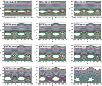
We consider RMP amplitudes in the range $0.1\ \text {mT}\leq \delta B_{r}\leq 2\ \text {mT}$ and examine the plasma properties at $t=5000\tau _A$, which we found was sufficient for the plasma response to reach a quasi-steady state. This was determined by examining the growth rate of the kinetic energy. Poincaré sections taken at $t=5000\tau _A$ for each $\delta B_{r}$ considered are shown in figure 6 as a function of poloidal angle and normalised poloidal flux. As expected, when the amplitude of the applied RMP is small ($0.1\ \text {mT}\leq \delta B_{r} \leq 0.5\ \text {mT}$), we observe saturation of an $(m=2,n=1)$ magnetic island at the $q=2$ surface, that is driven by the externally applied magnetic field.

Figure 6.

Poincaré sections of the plasma response as computed by M3D-C$^{1}$ and evaluated at $t=5000\tau _A$ for $0.1\ \text {mT}\leq \delta B_{r}\leq 2\ \text {mT}$. Shown here as a function of normalised poloidal flux, $\psi _p$, and poloidal angle, $\theta$.

For intermediate values, where $0.6\ \text {mT}\leq \delta B_{r} \leq 0.9\ \text {mT}$, we see the formation of secondary island chains about the O-points of the primary $(m=2,n=1)$ magnetic island chain. For example, for $\delta B_{r}=0.7$ mT, we see a secondary $m=9$ island chain. As the perturbation amplitude increases and the secondary islands grow larger, nonlinear interactions begin to drive significant chaos, leading to break up of the separatrix associated with the primary $(m=2,n=1)$ island. 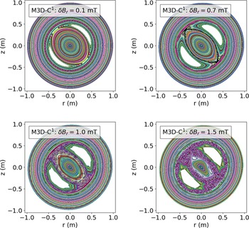For sufficiently large perturbation amplitudes ($\delta B_{r}\geq 1\ \text {mT}$), the primary $(m=2,n=1)$ island becomes embedded in, and eventually consumed by, a sea of chaos. In figure 7, we show a selection of Poincaré sections in $r-z$ coordinates which illustrate the different qualitative features associated with the nonlinear plasma response for varying $\delta B_{r}$. Namely, (i) a saturated $(m=2,n=1)$ magnetic island ($\delta B_{r}=0.1\ \text{mT}$), (ii) formation of secondary island chains ($\delta B_{r}=0.7\ \text{mT}$), (iii) break up of the separatrix associated with the primary $(m=2, n=1)$ island ($\delta B_{r}=1\ \text{mT}$) and, finally, (iv) near-complete stochasticisation of the plasma core ($\delta B_{r}=1.5\ \text{mT}$).

Figure 7.

Poincaré sections of the plasma response as computed by M3D-C$^{1}$ and evaluated at $t=5000\tau _A$ for $\delta B_{r}=0.1,\ 0.7,\ 1,\ 1.5\ \text{mT}$. The pressure profiles shown in figure 8 correspond to cuts taken along $z=0$.

The corresponding pressure profiles taken at a cut along $z=0$ when $t=5000\tau _A$ are shown in figure 8. Overlaid for comparison are the discretised pressure profiles used in the SPEC calculations, with $\varPsi _{t,i=3}=0.3$, $0.4$ and $0.5$. As expected, for $0.1 \text {mT}\leq \delta B_{r} \leq 1.5\ \text {mT}$ we find significant flattening of the pressure profile in regions coinciding with the $(m=2,n=1)$ magnetic island. Nonetheless, in all these cases we observe the presence of pressure gradients in regions coinciding with the $(m=2,n=1)$ island and magnetic field line chaos. This is attributable to the fact that the M3D-C$^{1}$ model accommodates finite perpendicular heat conductivity, where $\kappa _{\parallel }/\kappa _t\gg 1$. On the other hand, in the MRxMHD model there is assumed to be no perpendicular heat diffusion. As a consequence, pressure gradients cannot be supported across magnetic islands or in regions of magnetic field line chaos. It is to be expected that the SPEC and M3D-C$^{1}$ results will diverge when the effect of finite perpendicular heat conductivity becomes significant, although the differences may diminish for $\kappa _{\parallel }/\kappa _t$ significantly larger than the value considered in this work (Hudson Reference Hudson2009).

Figure 8.

Pressure profiles at $t=5000\tau _A$ as computed by M3D-C$^{1}$ shown as a cut taken along $z=0$ for $\delta B_{r}= 0.1,\ 0.7,\ 1,\ 1.5\ \text{mT}$ (solid lines). Also shown is the equilibrium pressure profile (black line), given by (2.2). For comparison, the discretised pressure profiles used in the SPEC calculations are represented by filled curves for $\varPsi _{t,i=3}=0.3$ (red), $0.4$ (green) and $0.5$ (blue).

5.2. Properties of the RMP response calculated with SPEC

As in § 5.1, we start from the initial axisymmetric equilibrium given by (2.1) and (2.2) and, this time, use the procedure described in § 3 to calculate MRxMHD solutions to an $(m=2,n=1)$ perturbation of the plasma boundary, with amplitude $\Delta r_a$. Specifically, we consider $0.01\ \text {mm}\leq \Delta r_a< 20\ \text {mm}$ which, using (4.20), corresponds to $0.0053\ \text {mT}\leq \delta B_{r}<1\ \text {mT}$. As discussed in § 3, we considered a fixed number of volumes, $N_{\rm vol}=5$, which is representative of practical use cases for the code, including in the context of modelling experimental measurements.

A key parameter for SPEC calculations is the amount of normalised toroidal flux, $\varPsi _{t,i}$, in each $i$th volume. This parameter has two important consequences. Firstly, the flux in each volume (which is held fixed during every SPEC solve) impacts the position of the interfaces in real space. This controls the spatial locations at which the original equilibrium profiles are discretised and, in turn, affects the fidelity of the discrete representation that is used by SPEC. This is particularly true for cases where $N_{\text{vol}}$ is relatively small, as is considered presently.

As will be seen, the value of $\varPsi _{t,i}$ in the volume containing the resonant surface of interest also has a strong effect on the properties of the magnetic islands that are computed by SPEC. In particular, the island width depends strongly on $\varPsi _{t,i}$ in the volume of interest, which is consistent with what has been observed previously in SPEC calculations performed in a slab geometry (Loizu et al. Reference Loizu, Hudson, Bhattacharjee and Helander2015).

We also find that the relative position, with respect to $\varPsi _{t,i}$, of the resonant surface of interest within the volume affects the shape of the resultant islands. Specifically, where the resonant surface is closer to one of the two bounding interfaces than the other (in terms of enclosed toroidal flux), the islands become distorted and deviate from the physically expected result. Therefore, for this study we took particular care to ensure that the $q=2$ resonant surface (which lies in the third volume) was centred with respect to $\varPsi _{t,i=3}$. This was achieved by carefully prescribing the value of $\iota =1/q$ for each interface in the ‘fixed iota’ step of the calculation procedure (see figure 5) and amounts to a particular discretisation of the $q$-profile. While possible in this work, the procedure adopted here may not be universally applicable because, in the general 3-D setting, the MRxMHD model requires interfaces to be associated only with surfaces that have sufficiently irrational $\iota$, in the sense of KAM theory. Since the existence of these KAM invariant tori is closely related to the shape of the surfaces (McGann et al. Reference McGann, Hudson, Dewar and von Nessi2010), the discretisation of the $q$-profile in the most general case is effectively fixed by the geometry of the problem.

5.3. Comparing the nonlinear RMP response in SPEC

In figure 9 we compare the island widths obtained from M3D-C$^{1}$ and SPEC for $\varPsi _{t,i=3}=0.3,0.4$ and $0.5$. The shaded regions correspond to the error bars associated with measurement of the island widths, which are obtained from field line tracing and examination of the Poincaré sections. As seen in figure 6, for $\delta B_{r}\geq 0.6\ \text {mT}$ we begin to observe significant stochasticisation of the separatrix associated with the primary $(m=2,n=1)$ island chain in M3D-C$^{1}$. In these cases, the island ‘widths’ shown in figure 9 are calculated by considering the distance between the two nearest flux surfaces bounding the islands and/or chaotic volume. Clearly, for $\delta B_{r}=2\ \text {mT}$ where we observe complete stochasticisation of the plasma core (figure 6, bottom right), no such quantity can be calculated.

Figure 9.

Saturated widths of $(m=2,n=1)$ magnetic islands due to externally applied $(2,1)$ RMP fields, as calculated by M3D-C$^{1}$ (pink), and SPEC for $\varPsi _{t,i=3}=0.3$ (blue), $\varPsi _{t,i=3}=0.4$ (orange) and $\varPsi _{t,i=3}=0.5$ (purple), where $\varPsi _{t,i=3}$ is the normalised toroidal flux enclosed in the volume containing the $q=2$ surface.

As already alluded to, in figure 9 we find a strong dependence of the SPEC island widths on $\varPsi _{t,i=3}$, the normalised toroidal flux in the volume containing the $q=2$ rational surface. Increasing $\varPsi _{t,i=3}$ in SPEC allows for larger islands as the strength of the RMP increases. This is to be expected since the maximum possible width of the island is only what can be allowed based on the toroidal flux initially enclosed in the volume. As can be seen for $\varPsi _{t,i=3}=0.3$ and $0.4$, if $\varPsi _{t,i}$ is too small the size of the resultant islands is artificially limited. For $\delta B_{r}\leq 0.5\ \text {mT}$, we observe the best overall agreement across this range of $\delta B_{r}$ when $\varPsi _{t,i=3}=0.5$. 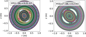In figure 10 we present an example of one such case (with $\delta B_{r}\approx 0.2 \text {mT}$) showing good agreement between the SPEC and M3D-C$^{1}$ calculations of the plasma response, which consists of a saturated $(m=2,n=1)$ magnetic island at the $q=2$ resonant surface. For the SPEC calculation, $N_{\rm vol}=5$ and $\varPsi _{t,i=3}=0.5$, while the M3D-C$^{1}$ solution is evaluated at $t=5000\tau _A$.

Figure 10.

Poincaré sections of the plasma response as computed by SPEC (left, $\delta B_{r}=0.21 \text { mT}$ and $\varPsi _{t,i=3}=0.5$) and M3D-C$^{1}$ (right, $\delta B_{r}=0.2 \text { mT}$). The SPEC interfaces are represented by black curves with $N_{\rm vol}=5$ and the M3D-C$^{1}$ solution is evaluated at $t=5000\tau _A$.

At very small RMP amplitudes, particularly below $\delta B_{r}\sim 0.05\text { mT}$, there is insufficient information in this study to conclusively determine which value of $\varPsi _{t,i=3}$ gives the best agreement between SPEC and M3D-C$^{1}$. This underscores an overarching observation, which is the sensitivity of the island properties as calculated by SPEC to the value of $\varPsi _{t,i=3}$. Because of the freedom that (to varying degrees) exists to prescribe $\varPsi _{t,i}$, this effect is especially important when SPEC is used to calculate quantitative island properties, such as in recent applications of the code to stellarator optimisation (Landreman et al. Reference Landreman, Medasani, Wechsung, Giuliani, Jorge and Zhu2021).

Particularly for $\varPsi _{t,i=3}=0.5$, we observe that the SPEC island widths, $w$, scale approximately as $\delta B_{r}^{1/2}$ for the values of $\delta B_{r}$ considered. According to theory (Wesson & Campbell Reference Wesson and Campbell2011), this implies that the resonant component of the total magnetic field at the $q=2$ surface, $\delta B$, remains linearly proportional to $\delta B_{r}$, the driving field at the plasma edge.

There are two conditions under which we expect island width to scale differently to $\delta B_{r}^{1/2}$. The first is when the island size is no longer small compared with equilibrium scale lengths such as the minor radius. From figure 7, we see that significant islands can open up in the M3D-C$^{1}$ solution, even for $\delta B_r=0.1 \text { mT}$. It is expected that the inclusion of equilibrium flows would lead to a significant reduction of the island size. While M3D-C$^{1}$ can accommodate states with equilibrium flows, work to extend the MRxMHD model to incorporate flows is ongoing. Consequently, we were limited to the static version of the MRxMHD model for this study and, therefore, do not consider the effect of equilibrium flows.

The island width scaling can also be modified when the resonant component of the field at the $q=2$ surface is no longer linearly proportional to the driving field, i.e. no longer satisfying $\delta B\propto \delta B_r$. This is indicative of significant nonlinearity in the plasma response, such as shielding or amplification of the applied RMP field. At larger $\delta B_{r}$, figure 9 suggests that for $\varPsi _{t,i=3}=0.5$ the response computed by SPEC remains largely linear insomuch that $\delta B\propto \delta B_r$ since $w\propto \delta B_{r}^{1/2}$. In contrast, solutions calculated by the M3D-C$^{1}$ model, which has been extensively validated and used to model the plasma response (both linear and nonlinear) to externally applied 3-D fields in a range of applications (Ferraro et al. Reference Ferraro, Evans, Lao, Moyer, Nazikian, Orlov, Shafer, Unterberg, Wade and Wingen2013; Reiman et al. Reference Reiman, Ferraro, Turnbull, Park, Cerfon, Evans, Lanctot, Lazarus, Liu, McFadden, Monticello and Suzuki2015; Wingen et al. Reference Wingen, Ferraro, Shafer, Unterberg, Canik, Evans, Hillis, Hirshman, Seal, Snyder and Sontag2015; Canal et al. Reference Canal, Ferraro, Evans, Osborne, Menard, Ahn, Maingi, Wingen, Ciro, Frerichs, Schmitz, Soukhanoviskii, Waters and Sabbagh2017; Lyons et al. Reference Lyons, Ferraro, Paz-Soldan, Nazikian and Wingen2017), shows a clear deviation from the square-root scaling at larger $\delta B_{r}$. This suggests that nonlinear mechanisms, leading to shielding and/or amplification of the applied RMP field, contribute significantly to the plasma response. While beyond the scope of the present work, further elucidating the physics properties of the plasma response predicted by the MRxMHD model would be valuable as part of future work. In particular, examining the resonant component of the magnetic field at the corresponding rational surface to identify linear and nonlinear contributions to the plasma response.

5.4. Robustness and sensitivity of SPEC solutions

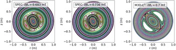
SPEC uses Newton methods to solve for both the Beltrami fields (3.1) and the interface geometry (3.2) and, as a consequence, can become sensitive to small changes in parameters such as $\Delta r_a$. We observed this to be the case for larger perturbation amplitudes, where $\delta B_{r}>0.5\ \text {mT}$. An example of this is illustrated in figure 11. As in figure 10, $N_{\rm vol}=5$ and $\varPsi _{t,i=3}=0.5$ in the SPEC calculation, while the M3D-C$^{1}$ solution is evaluated at $t=5000\tau _A$. For $\delta B_{r}=0.7\ \text{mT}$, the plasma response obtained from M3D-C$^{1}$ is charact- erised by a saturated $(m=2,n=1)$ island at the $q=2$ resonant surface and about which there is a higher $m$ secondary island chain. In contrast, for ${\delta B_{r}=0.683 \text {mT}}$ and $\delta B_{r}=0.736 \text { mT}$, which differ only slightly, we observe two qualitatively different solutions for the plasma response as calculated by SPEC, both of which differ from the M3D-C$^{1}$ response. In particular, for $\delta B_{r}=0.736 \text { mT}$ we observe the appearance of a high $m$ island chain in an inner volume which does not contain the $q=2$ resonant surface.

Figure 11.

Poincaré sections of the plasma response as computed by SPEC (left, $\delta B_{r}=0.683 \text { mT}$ and $\varPsi _{t,i=3}=0.5$) and (centre, $\delta B_{r}=0.736 \text { mT}$ and $\varPsi _{t,i=3}=0.5$) and M3D-C$^{1}$ (right, $\delta B_{r}=0.7 \text { mT}$). The SPEC interfaces are represented by black curves with $N_{\rm vol}=5$ and the M3D-C$^{1}$ solution is evaluated at $t=5000\tau _A$.

As a measure of robustness, we consider the residual force error which represents the net force on each interface and, therefore, the difference between the numerical solution and the equilibrium condition, (3.2). For $\delta B_{r}\leq 0.5\ \text {mT}$, at fixed Fourier resolution, the force error is $O(10^{-12})$ or less and, for $\varPsi _{t,i=3}=0.5$, we find good agreement between SPEC and M3D-C$^{1}$ (see figure 9). However, at the same Fourier resolution, for $\delta B_{r}\geq 0.6\ \text {mT}$ we find that the force error becomes very sensitive to small changes in $\Delta r_a$. In this regime, we observed that even when the force error was at most $O(10^{-13})$, a change of $\Delta r_a=0.1\ \text{mm}$ could be sufficient to yield solutions with qualitatively different characteristics, e.g. a single $(m=2,n=1)$ island chain vs. islands embedded in a chaotic sea.

One strategy for reducing sensitivity is to choose an initial guess that is close to the desired solution. This may be achieved, for example, by starting from an axisymmetric solution and constructing a sequence of solutions while incrementally increasing a parameter of interest (such as $\Delta r_a$) until the desired value is reached. Such an approach requires the calculation of a large number of solutions, which is time consuming and, thus, not a universally viable strategy.

The observed decrease in robustness in the strongly driven RMP regime ($\delta B_{r}>0.5\ \text {mT}$) has important implications for applications including stellarator optimisation, where SPEC may be used to calculate quantitative properties of the equilibrium magnetic field structure. The ability to efficiently and reliably compute physics properties is essential for plasma optimisation procedures. In practice, parameters such as Fourier resolution are commonly specified in advance and held fixed during an optimisation run. On the other hand, $\Delta r_a$, which is related to the boundary shape, can change significantly in a free-boundary optimisation. We have seen, however, that the robustness of SPEC solutions can depend sensitively on both parameters.